Causal effect estimation in sequencing studies: a Bayesian method to account for confounder adjustment uncertainty

(1)

P R O C E E D I N G S

Open Access

Causal effect estimation in sequencing

studies: a Bayesian method to account for

confounder adjustment uncertainty

Chi Wang

1,2

, Jinpeng Liu

2

and David W. Fardo

1*

FromGenetic Analysis Workshop 19 Vienna, Austria. 24-26 August 2014

Abstract

Estimating the causal effect of a single nucleotide variant (SNV) on clinical phenotypes is of interest in many genetic studies. The effect estimation may be confounded by other SNVs as a result of linkage disequilibrium as well as demographic and clinical characteristics. Because a large number of these other variables, which we call potential confounders, are collected, it is challenging to select and adjust for the variables that truly confound the causal effect. The Bayesian adjustment for confounding (BAC) method has been proposed as a general method to estimate the average causal effect in the presence of a large number of potential confounders under the assumption of no unmeasured confounders. In this paper, we explore the application of BAC in genetic studies using Genetic Analysis Workshop 19 exome sequencing data. Our results show that BAC can efficiently estimate the causal effect of genetic variants with adjustment for confounding. Consequently, BAC may serve as a useful tool for genome-wide association studies data analysis to effectively assess the causal effect of genetic variants and the impact of potential interventions.

Background

In genetic studies, a large number of baseline and gen-etic variables are observed. The selection and adjustment of these covariates is essential for estimating the average causal effect (ACE). Recently, a method called Bayesian adjustment for confounding (BAC) [1, 2] was proposed to account for the uncertainty in confounder selection while estimating the ACE of a certain exposure variable. BAC uses a Bayesian model averaging (BMA) [3] ap-proach to estimate the ACE by taking a posterior weighted average of ACE estimates from a battery of models with adjustments of different sets of covariates. A key feature of BAC is that it incorporates the strength of associations between covariates in the model and the exposure into the prior for each individual model. This is different from the regular BMA method, which assigns

uniform prior weight to each model. It has been shown that large posterior weights in BAC are usually given to models that have fully adjusted for confounding so that an unbiased estimate of ACE can be obtained.

In this paper, we explore the application of BAC in estimating the ACE of single-nucleotide variants (SNVs). Although BAC has been applied to environmental and clinical studies [1, 2], to our knowledge, this is the first time for this method to be applied to genetic studies. We illustrate the application of BAC using Genetic Analysis Workshop 19 (GAW19) sequencing data. Briefly, these data consist of hg19-aligned whole exome sequences from 1943 unrelated Hispanic subjects as part of Type 2 Diabetes Genetic Exploration by Next-generation sequencing in Ethnic Samples (T2D-GENES) Project 1. We focus on evaluating the causal effect of SNVs inMAP4 and utilize the 200 simulated phenotype sets from these individuals [4].

* Correspondence:[email protected]

1_{Department of Biostatistics, College of Public Health, University of Kentucky,}

725 Rose St, Lexington, KY 40536, USA

Full list of author information is available at the end of the article

(2)

Methods The causal model

We adopt the Rubin causal model [5, 6] to estimate the ACE of a certain SNV, which we call the exposure, on systolic blood pressure (SBP), which we call the out-come. Let Y(X) be the potential outcome an individual would have if the genotype was X. Here, we assume an additive mode of inheritance so that Xis the number of alternative alleles, ie,X∈{0, 1, 2}. The observed outcome Y is the outcome associated with an individual’s actual genotype: Y=∑x2= 0Y(x)I{X=x}, where I{X=x} is one if

the individual’s genotype is x or zero otherwise. Thus, the ACE for having one alternative allele isΔ=E{Y(1)}− E{Y(0)}. Suppose the true set of confounders,U*, can be identified. Under the strong ignorability assumption [7], which assumes the potential outcomes and X are inde-pendent givenU*,E{Y(x)} =E{E(Y|X=x, U*)}. Therefore,

Δ=E{E(Y|X= 1, U*)}− E{E(Y|X= 0, U*)}. If we further assume a linear regression model forY onX and U*, it can be shown that the ACE is equal to the correspond-ing model coefficient ofX.

In practice, however, it is usually uncertain which co-variates are true confounders. This is particularly chal-lenging in genetic association studies where many variants are correlated and the true causal variants are unknown. The bias and variance of the ACE estimate can depend strongly on which covariates are included for adjustment in the analysis. To deal with this prob-lem, we propose the following approach.

The Bayesian adjustment for confounding method LetU= {U1, ⋯,UM} be the set of potential confounders. We assume no unmeasured confounders so thatU⊇U*. To adjust for confounders and estimate the ACE, we jointly consider two models: a logistic regression model for the SNV of interest (the exposure model) and a linear regression model for the outcome (the outcome model). Specifically,

outcome models, respectively; m indexes SNVs and i indexes individuals. For convenience, we refer to param-eter vectors αX= (α1X,⋯,αMX)T and αY= (α1Y,⋯,αMY)T as

“models.” For regression coefficients,β and δ, we use a notation that explicitly keeps track of the fact that these coefficients differ in meaning with the αs. Furthermore,

to clarify the estimand, it is useful to consider the smal-lest outcome model that includes all the true con-founders. We denote that model by α*Y. Our estimand,

the ACE ofX onY, is the coefficient ofX inα*Y, denoted

byβ*.

As α*Y is usually unknown, we use a Bayesian model

averaging approach to obtain the posterior ofβ*by taking

a weighted average across the posteriors under each pos-sible model: model that contains α*Y (meaning that the model

in-cludes all the covariates inα*Y), its model coefficient ofX

is also equal toβ*. For a model that does not containα*Y,

its model coefficient ofXmay be different fromβ*.

Con-sequently, the approximation works well if the model weight p(αY|D) concentrates on models that containα*Y.

Otherwise, it can be largely biased from the inclusion of models not fully adjusted for confounders.

To ensure large weights are assigned to models that containα*Yand based on the fact that confounders are

ne-cessarily associated with bothXandY, we propose to ob-tain the posterior ofαYby pðαYjDÞ ¼X_α_XpαX;αYjD, where the joint posterior of αX and αY is calculated by assuming the following prior: 1, it increases the chance for a covariate associated with

Xto be included into the outcome model. Such a covari-ate, if also associated withY, is likely to be a confounder. Therefore, the above prior facilitates confounder selec-tion by advocating the use of a covariate’s associations with both the exposure and the outcome to determine its inclusion in or exclusion from the outcome model. It is likely to yield a posterior of αYthat assigns mass preferentially to models including all the true con-founders [2].

(3)

that implement BAC are available at http://sweb.uky. edu/~cwa236/BAC_GAW19.zip.

Data sets and data filtering

We consider GAW19 sequencing data, which consist of hg19-aligned whole exome sequences from 1943 unre-lated Hispanic subjects, as part of T2D-GENES Project 1. The corresponding phenotypic data are from the 200 simulated phenotypic data sets (including the null Q1 trait) generated by GAW19. Because of the lack of age information, 81 subjects are dropped. We focus on the SNVs in the MAP4 gene as well as those 5 kb up- or downstream ofMAP4. SNVs that have either zero minor allele frequency (MAF) or low coverage (<20×) are fil-tered out, which leaves a total of 94 SNVs. Among those SNVs, 25 have true effects on SBP in the simulation model.

Results

We evaluated the performance of BAC by using the GAW19 sequencing data after applying the filtering as

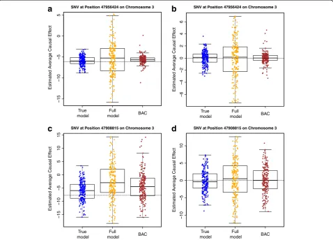
described in the Methods section. We considered SBP as the outcome and evaluated the estimation of ACE for two SNVs in the MAP4 gene: 1 common SNV at pos-ition 47956424, chromosome 3 (MAF = 0.3435) and one rare SNV at position 47908815, chromosome 3 (MAF = 0.0026). The set of potential confounders include age, sex, their interaction, smoking status, and all the SNVs (other than the SNV of interest) in MAP4 as well as those 5 kb up- or downstream of MAP4. We applied BAC to the set of potential confounders to automatically select and adjust for confounders and to estimate the ACE. We set the dependence parameter ω equal to ten because it appears to provide a good balance between in-cluding important confounders and exin-cluding variables only associated with the exposure based on our previous experience. For comparison, we considered the “true model,” which includes age, sex, their interaction, and the 25 SNVs with true effects, and the “full model,” which includes all the potential confounders. Figure 1 and Table 1 summarize the results. In all scenarios, the standard error of ACE estimates based on BAC is

15

10

50

5

SNV at Position 47956424 on Chromosome 3

a

b

Estimated A

Fig. 1ACE estimates. ACE estimates based on the“true model,”the“full model”and BAC for twoMAP4SNVs at position 47956424 (aandb) and

position 47908815 (candd) on chromosome 3.aandcare based on 200 simulated phenotypic data sets;banddare based on 200 Q1 data sets. The

(4)

smaller than that based on the “full model.” As an example, for the ACE estimation of SNV 47956424 by using simulated phenotypic data, the sample standard error based on BAC is 1.277, which is much smaller than the value 4.280 based on the “full model” and is close to the value 1.121 based on the “true model.” The root mean square error (RMSE) based on BAC is also smaller than that based on the “full model.” Therefore, by performing variable selection and model averaging, BAC is able to effectively reduce the variation and yield a more precise estimate of the ACE.

Discussion

BAC jointly considers an exposure model and an out-come model, which enables proper selection and adjust-ment for confounders and yields significantly reduced variation in ACE estimation. For simplicity, the exposure model we consider in the paper is a logistic regression model, where the genotype of the exposure is dichoto-mized into containing at least one alternative allele or not. One may extend the BAC method by considering a polytomous regression model for the exposure model, where the number of alternative alleles can be taken into account. However, because the exposure model is only used to identify important confounders to be adjusted and the causal effect is estimated based on the outcome model, BAC is relatively robust to the misspecification of the exposure model as long as confounder identifica-tion is not largely affected.

The dependence parameter ω indicates the prior strength of connection between the exposure and the outcome models. On the one hand, setting ω equal to one assumes no connection between the two models.

Thus, the associations between potential confounders and the exposure will not be accounted for in the vari-able selection procedure, which may bias the ACE esti-mation. One the other hand, settingωequal to ∞forces all potential confounders that are in the exposure model to be included in the outcome model. Thus, variables that are only associated with the exposure but not with the outcome may be included in the outcome model and inflate the variation of ACE estimation. Therefore, we recommend choosing a finiteω value that can achieve a nice balance between bias and variation. Based on our previous experience, settingωequal to ten works well in simulation scenarios. A more sophisticated method to determine the optimalω value can be found in Lefebvre et al. [9].

Conclusions

The primary goal of genetic association analysis is detec-tion of variants that correlate with some disease pheno-type. Replicable associations between variants and many diseases and related endophenotypes have been discov-ered and subsequently followed with functional studies. While insight into biological function supersedes this primary goal of association study, as substantiated by the era of candidate gene studies, these insights must be pursued for complex disease associations.

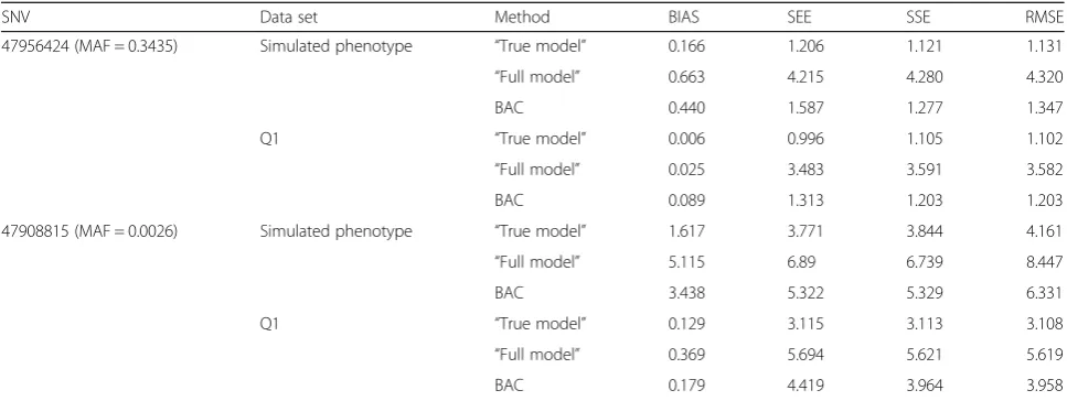
The BAC method employed here aims to estimate the causal effect of genetic variants on disease phenotype. These effect metrics represent an attempt to bridge the gap between association and function, while improving the localization of disease-correlated variants. This paper demonstrates that BAC is able to appropriately estimate the causal effect and handle the complexity in the Table 1Estimation results. Estimation of the ACE on SBP for twoMAP4SNVs at position 47956424 and position 47908815,

chromosome 3

SNV Data set Method BIAS SEE SSE RMSE

47956424 (MAF = 0.3435) Simulated phenotype “True model” 0.166 1.206 1.121 1.131

“Full model” 0.663 4.215 4.280 4.320

BAC 0.440 1.587 1.277 1.347

Q1 “True model” 0.006 0.996 1.105 1.102

“Full model” 0.025 3.483 3.591 3.582

BAC 0.089 1.313 1.203 1.203

47908815 (MAF = 0.0026) Simulated phenotype “True model” 1.617 3.771 3.844 4.161

“Full model” 5.115 6.89 6.739 8.447

BAC 3.438 5.322 5.329 6.331

Q1 “True model” 0.129 3.115 3.113 3.108

“Full model” 0.369 5.694 5.621 5.619

BAC 0.179 4.419 3.964 3.958

BIAS is the difference between the mean of estimates of ACE and the true value; RMSE is the root mean square error; SEE is the mean of standard error estimates; SSE is the standard error of the estimates of ACE

(5)

adjustment of confounding as a result of linkage disequi-librium. Our finding that BAC provides a more efficient ACE estimate than conventional methods suggests that BAC has the potential to be widely applied to genome-wide association studies data to effectively assess the causal effect of genetic variants and the impact of poten-tial interventions.

Declarations

This work was partially supported by the National Institute on Aging (DWF: K25AG043546). The Genetic Analysis Workshop is supported by National Institutes of Health (NIH) grant R01 GM031575. The GAW19 whole genome sequence data were provided by the T2D-GENES Consortium, which is supported by NIH grants U01 DK085524, U01 DK085584, U01 DK085501, U01 DK085526, and U01 DK085545. The other genetic and phenotypic data for Genetic Analysis Workshop 18 were provided by the San Antonio Family Heart Study and San Antonio Family Diabetes/Gallbladder Study, which are supported by NIH grants P01 HL045222, R01 DK047482, and R01 DK053889. The Genetic Analysis Workshop is supported by NIH grant R01 GM031575.

This article has been published as part ofBMC ProceedingsVolume 10

Supplement 7, 2016: Genetic Analysis Workshop 19: Sequence, Blood Pressure and Expression Data. Summary articles. The full contents of the supplement are available online at http://bmcproc.biomedcentral.com/ articles/supplements/volume-10-supplement-7. Publication of the proceedings of Genetic Analysis Workshop 19 was supported by National Institutes of Health grant R01 GM031575.

Authors_’contributions

CW and DWF conceived and designed the study, JL and CW performed the analyses, and CW and DWF wrote the manuscript. All authors discussed results and their implications and commented on the manuscript at all stages. All authors read and approved the final manuscript.

Competing interests

The authors declare that they have no competing interests.

Author details 1

Department of Biostatistics, College of Public Health, University of Kentucky, 725 Rose St, Lexington, KY 40536, USA.2_{Biostatistics and Bioinformatics}

Shared Resource Facility, Markey Cancer Center, University of Kentucky, 800 Rose St, Lexington, KY 40536, USA.

Published: 18 October 2016

References

1. Lefebvre G, Delaney JA, McClelland RL. Extending the Bayesian adjustment

for confounding algorithm to binary treatment covariates to estimate the effect of smoking on carotid intima-media thickness: the Multi-Ethnic Study

of Atherosclerosis. Stat Med. 2014;33(16):2797–813.

2. Wang C, Parmigiani G, Dominici F. Bayesian effect estimation accounting for

adjustment uncertainty. Biometrics. 2012;68(3):661–71.

3. Raftery AE, Madigan D, Hoeting JA. Bayesian model averaging for linear

regression models. J Am Stat Assoc. 1997;92(437):179–91.

4. Blangero J, Teslovich TM, Sim X, Almeida MA, Jun G, Dyer TD, Johnson M,

Peralta JM, Manning AK, Wood AR, et al. Omics squared: human genomic, transcriptomic, and phenotypic data for Genetic Analysis Workshop 19. BMC Proc. 2015;9 Suppl 8:S2.

5. Rubin DB. Estimating causal effects of treatments in randomized and

nonrandomized studies. J Educ Psychol. 1974;66(5):688–701.

6. Rubin DB. Assignment to treatment group on the basis of a covariate.

J Educ Behav Stat. 1977;2(1):1–26.

7. Rosenbaum PR, Rubin DB. The central role of the propensity score in

observational studies for causal effects. Biometrika. 1983;70(1):41–55.

8. Madigan D, York J, Allard D. Bayesian graphical models for discrete data.

Int Stat Rev. 1995;63(2):215–32.

9. Lefebvre G, Atherton J, Talbot D. The effect of the prior distribution in the

Bayesian adjustment for confounding algorithm. Comput Stat Data Anal.

2014;70:227_–40.

• We accept pre-submission inquiries

• Our selector tool helps you to find the most relevant journal • We provide round the clock customer support

• Convenient online submission • Thorough peer review

• Inclusion in PubMed and all major indexing services • Maximum visibility for your research

Submit your manuscript at www.biomedcentral.com/submit