Edge function method applied to thin plates resting on Winkler foundation

EDGE FUNCTION METHOD APPLIED TO

THIN PLATES RESTING ON WINKLER FOUNDATION

Thesis by

Ignatius Po-cheung Lam

In Partial Fulfillment of the Requirements for the D-egree of

Civil Engineer

California Institute of Technology Pasadena, California

1976

The writer would like to express his appreciation for the guidance

and assistance offered by Professor R. Scott throughout the course of

this investigation.

The writer is also indebted to Professor G. W. Housner for

read-ing the first draft and valuable criticism;· to Mr. D. Dhar, currently a

physics graduate student at the California Institute of Technology for his

suggestions.

ABSTRACT

The Edge Function method formerly developed by Quinlan (ZS) is

applied to solve the problem of thin elastic plates resting on spring

supported foundations subjected to lateral loads the method can be

applied to plates of any convex polygonal shapes, however, since most

plates are rectangular in shape, this specific class is investigated in

this thesis. The method discussed can also be applied easily to other

kinds of foundation models (e. g. springs connected to each other by a

membrane) as long as the resulting differential equation is linear.

In chapter VII, solution of a specific problem is compared with a known

solution from literature. In chapter VIII, further comparisons are given.

The problems of concentrated load on an edge and later on a corner of a

plate as long as they are far away from other boundaries are also given

in the chapter and generalized to other loading intensities and/or plates

I

springs constants for Poisson s ratio equal to O. 2 •

CHAPTER

I

n

III

IV

v

VI

VII

VIII

IX

TITLE PAGE

HISTORICAL BACKGROUND ••••••••••..•••. 1

FORMULATION OF PROBLEM AND

PARTICULAR SOLUTION ADOPTED .•••••• 9

EDGE FUNCTION METHOD ••••••.•••••••••• 16

EDGE FUNCTION METHOD FOR

A RECTANGULAR PLATE ON

WINKLER FOUNDATION .•••••••••••••••• 21

CONVERGENCE ••.••.••.•.•••••••••••••••• 3 0

SYMMETRICAL PROPERTIES •••.•.•••••••• 35

CONCLUSION AND EXAMPLES •••.••••••.•• 44

ITERATIVE METHOD AND FURTHER

EXAMPLES . . . ·· . . . 55

COMPARISON WITH OTHElt

AVAILABLE METHODS ••••••••.••••••••• 74

APPENDICES . . . · . . . • . . . 80

REFERENCES . . . 107

-1-CHAPTER I. HISTORICAL BACKGROUND

The problem of deflection of an elastically supported elastic plate has become important since the introduction of concrete paving slabs for roads and aircraft runways. During World War II, consid-erable activity took place in northern Canada and Alaska so that the problem of transporting heavy equipment over frozen lakes became important. The above problems, as well as the necessity to design raft foundations for buildings, have resulted in a great deal of re-search activity on the problem of a loaded elastic plate on various kinds of supporting medium.

Soils are in general nonlinear, nonhomogeneous and aniso-tropic, but it is frequently assumed that a soil mass can be

repre-sented by a semi-infinite linearly elastic medium. However, even this model renders the problem too hard to solve in most cases. For the sake of mathematical expedience the simplest model, equiv -alent to a bed of springs, was suggested by Winkler (l) and many papers have been written on the plate problem using this model. The following is a brief review of the literature dealing with the problem of a loaded elastic plate on Winkler 1

s model of a supporting medium.

Later in this chapter a review will also be given concerning other models.

The problem of deflection of an elastic plate resting on some kind of medium was first discussed by Winkler. (l) He proposed the simplest relationship between the local reaction of the supporting medium p and the local deflection • . He suggested that the pressure,

s

equivalent to the condition of a buoyant plate resting on a liquid, as

in the case, for example, of a floating ice sheet. The only reaction

of the subgrade is an upward force proportional to the deflection.

This description of a foundation reaction is frequently called a

"Winkler Foundation." Winkler used this model to study the behavior

of railroad rails resting on ties. It was also used by Hertz (40) in a

study of a floating ice sheet.

Westergaard(Z, 3) solved approximately the problem of an

in-finite or semi-inin-finite elastic thin plate resting on a Winkler

Founda-tion when the load is uniformly distributed first over a circle and

later an ellipse. He also gave some formulas for the maximum

ten-sile stresses developed in the plate. In the infinite plate problem,

the loading can be distributed uniformly over any area having both

axes of x andy as axes of symmetry. Westergaard's investigation

of tensile stresses had immediate application to the design of

high-ways and airfield pavements.

Wyman (4) solved analytically the problem of a point load on

an infinite thin plate resting on Winkler Foundation. The solution

he obtained was expr essed in terms of Bessel's functions. The point

load solution can be generalized, as shown by Wyman, to obtain

solu-tions for arbitrary loading condition. However, the solution is ex

-pressed in integral form and,in most cases, the integral is too hard

to evaluate. Wyman, however, applied the idea to a uniform circular

loading condition and evaluated the deflections • .

R. K. Livesley(S) obtained solutions to the problem of

-3-a double Fourier transform and expressed the solution as an integral. When an edge or edges are simply supported, the solution can be ex-tended to semi-infinite plates or plates of the shape of an infinite

quadrant. He also obtained solutions for a semi-infinite plate on a Winkler Foundation loaded by prescribed moments and shear stress normally along the edge of the plate. Dynamical loading is also

dis-cussed in the paper.

Other than the above papers, Kerr(6) solved the problem of a simply suppo~ted wedge -shaped plate, not supported by any founda-tion, subjected to uniform tension in the plane of the plate and loaded transversely by concentrated forces. The behavior of a loaded corner of the plate can be obtained from the results of the paper. In another paper, written by Kerr,(?) he tackled the problem of simply supported plates on a Winkler Foundation subjected to concentrated loads and obtained solutions for the following shapes of plates: (1) wedge-shaped; (2) infinite strip; (3) semi-infinite strip; (4) rectangular plate.

S. Timoshenko and Woinowsky-Krieger(B) included a chapter on the topic of plates on a Winkler Foundation. In that chapter, there are solutions to several problems, a very interesting one being

that of a rectangular plate simply supported on all four edges and loaded by any arbit:rary lateral loads. The solution is expressed as a double sine series. This is one of the very few exact solutions obtained for a finite plate on a Winkler Foundation.

Other than the above mentioned papers, Hetenyi (l6) has

Many examples are given in the book. However, the book deals mainly with beam rather than plate problems.

The problems of plates on a Winkler Foundation that have

been solved are mainly those of infinite, semi-infinite plates or

those plates with the shape of an infinite quadrant and are listed in

Table 1. 1.

The problem of a finite plate on a Winkler Foundation is very

complicated. Ther e is only one solution in the literature (chapter 8).(8)

From it, the solution of any arbitrary lateral load on a simply

sup-ported (hinged) rectangular plate can be obtained.

In addition to plates on the Winkler Foundations, many workers

have proposed different kinds of models for the supporting medium. Hogg(9) solved the problem of a thin infinite plate, symmetrically

loaded and resting on an elastic half-space. Then, in a later paper,

Hogg (l O) solved a similar problem in which the elastic foundation was of finite depth.

However, to make the problem more manageable, most inves

-tigations on a better foundation model have been carried out in one-dimension (a beam, instead of a plate}. For example, most compar-isons with experimental results have been made using a theoretical

solution of an elastic beam on a variety of foundation models. The foundation pressure p (x} is very often assumed to be proportional

s

to the displacement and/or various derivatives of displacements. This model is popular because the Winkler's model of foundation is completely discontinuous. If other derivatives are taken into

TABLE

1.1

Solved

Problems

of

Plates

on

a

Winkler

Foundation

Shape

of

Plate

Loading

Condition

Boundary

Conditions

a)

Point

Load

Solution

approaches

zero

b)

Loads

with

Circular

Infinite

as

it

is

infinitely

far

away

Symmetry

from

the

load

c)

Arbitrary

a)

Elliptical

Shapes

b)

Circular

and

Elliptical

Free

Edge

Semi-Infinite

Shapes

Infinite

Quadrant

c)

Arbitrar

y

Simply

Supported

a)

Arbitrary

Simply

Supported

~---.

-·

-Reference

@

®

!G),

@,

®

@

,

(I

@,

(5\

'-·

(~),@G)

taken into consideration. As mentioned earlier, in the Winkler Model p (x) is assumed to be proportional to the displacement only. But

s

in the most general linear case, it can be assumed to be expressed

by the following equation:

p _s

(x)

N

=

E

a w(n) (x)

n=O n

(1. 1)

in which w(n)(x) denotes the nth derivative of the deflection w(x) with respect to the x-direction. An extensive review of the literature in

this area is given in refs. (1), (11), (12), (13), (14), {15) and (16).

For example: Pasternak{l3) suggested the model:

ps{x) = k

1w(x)-k2w

11_{(x), whereas}

Hetenyi (l2) proposed the following model:

(1. 2)

(1. 3)

The Winkler Foundation(!) assumes complete lateral discon-tinuity in the elements in the foundation material, whereas the

half-space of Hogg( 9, 1 O) assumes complete continuity. Hetenyi' s (l ?)

equation (1. 3) and chapter 10(!6) used an arbitrary degree of

con-tinuity on the foundation and applied it successfully to the one-dimensional beam problem. However, it is doubtful whether this method could be applied to the two-dimensional plate equation. The reason for using this model, rather than the Winkler model, is that

it offers more parameters that one can choose to approximate the

actual elastic continuum. model.

-7-the parameters in their models. (for example, k

1 and k2 in the

Pasternak and Hetenyi Model described in eq. (1. 2) and (1. 3) ).

Fletcher and Hermann(lS) gave a systematic way to determine what

values of the parameters (constants) in the model represented by

eq. (1. 2) and (1. 3) should be used, if the elastic constants of the

(linearized isotropic) foundation material are known. Timoshenko

and Woinowsky-Krieger (p. 259)(8) give a table which gives engineers

the values of the Winkler constant that should be used for various

types of soil.

Other than the above -mentioned static models, Kerr (!5) has

suggested a time-dependent model in which a viscoelastic effect was

introduced. However, Kerr applied the model to a plate which can

only withstand transverse shear (a shear plate).

All of the solved problems involve a particular plate shape

and boundary conditions generally simply-supported at the edges.

For the general solution of slab problems even of moderate

com-plexity, numerical procedures have to be adopted. So far in the

literature, two methods have been used: the finite difference and

the finite element techniques. Allen, and Severn (19 ' 20) used the

finite difference method and reduced the solution to a system of

linear equation. However, in this formulation it is sometimes

dif-ficult to ini:-oduce the boundary conditions.

Zienkiewicz and Cheung(2l) and Severn (22) have applied the

finite element technique to the plate problem. The finite element

method is a versatile method that can deal with any boundary

usually uses a continuum model for foundation material, so it can

model any corn,bination of materials, layers, etc., but may be

ex-pensive.

Other investigators who have contributed to the problem are

I (23) (24)

Vlasov and Leont ev and Holl.

Among all the above -mentioned methods, only finite

differ-ence and finite element techniques can be used to handle the plate

problem with some generality. However, they are not without fault.

Their advantages and disadvantages will be compared and discussed

-9-CHAPTER II. FORMULATION OF THE PROBLEM

AND PARTICULAR SOLUTION ADOPTED

The foundation model that is adopted in this paper is the

Winkler Foundation. In view of all the uncertainty connected with

the soil property determination, it seems unjustifiable to use a more

sophisticated model which would make the problem much more

diffi-cult. However, if other models for the soil reaction are used, as

long as the differential equation involved is linear, the Edge Function

technique can still be applied.

(a) Formulation

When the plate is thin compared to other dimensions (e. g. the

radii of curvature of the sur face) of the plate and the deflection w of

the plate are small compared to the thickness of the plate, an approx

-imate theory of bending of the plate by lateral loads can be developed

by making the following assumptions:

1. There is no in-plane deformation in the middle surface

of the plate.

2. Points in the plate lying initially on a normal to middle

plane of the plate remain on the normal" after bending.

3. The normal strains in the direction transverse to the plate are negligibly small.

Using these assumptions, all stress components can be

ex-pressed in terms of the deflection w of the plate, which is a function

of the two coordinates in the plane of the plate. This function has to

satisfy a linear partial .differential equation, which, together with

solution of this equation gives all the information necessary for ca

l-culating stresses at any point of the plate. The equation of the plate

for any of the model foundation material is given by:

4 Ps (x, y)

'i1 w (x, y)

+

D

where

=

q(x, _D y) (2. I)

E and V are Young's modulus and Poisson's Ratio of the elastic plate.

h is the thickness of the plate.

q(~ y) is a function that describes the loading.

p _s is the foundation pressure

+

Adopting the Winkler model for the foundation, ps is given by

the following equation

where K is a constant.

p (x, y) = Kw(x, y)

s {2. 2)

Substituting eq. (I. 5) into (1. 4) the differential equation of

the deflected sur face is obtained as follows:

4

K

'i1 w(x, y)

+

D w (x, y) = q(x_D , y) (2. 3)

The above assumption and differential equations are basically adopted

-11-(b) Boundary Conditions

To make the solution unique, boundary conditions have to be

specified. In most engineering problems, the properties of interest

are among the following: displacement; slope; moment and shear.

The boundary conditions include specifying any two of the

above properties along each boundary. To express the above

prop-erties mathematically involving derivatives of displacement w, the

derivation in chapter 2 of ref. 8 is adopted and the results are listed

as follows:

a)

b)

displacement is given by w

ow

slope in the n direction is given by

on

c)

2 2

moment per unit length in the n direction is -D (8 w

+

'V 0 w)

an

2

at

2

3 3

shear force per unit length in then direction is -D(0 '; +(2-'V) 0 w

on

onot

d)

(2. 4)

where the coordinates are as given in Fig. 2. 1.

To solve the problem, the equation is broken down into two

parts to obtain: (1) The non-homogeneous solution; (2) The homo

g-enous solution.

(1) The non-homogeneous solution (particular solution).

From eq. (2. 3) the particular solution is given by

+

K w

D

p

=

q(x, y)

(2) The homogeneous solution (complementary solution) has to satisfy the following equation:

,.,4 w K

v c

+

D w _c

=

0 (2. 6)

w is adjusted such that together with the particular solution it will c

give a total solution, wt' that satisfies the loading and the boundary conditions. Details of the solution methods are given in the following chapters.

Then the total s elution is given by

w

=

w +w

t p c

any ) \

__.--'7

n

plane

~

Fig. 2. 1

~Boundary of

the Plate

(2. 7)

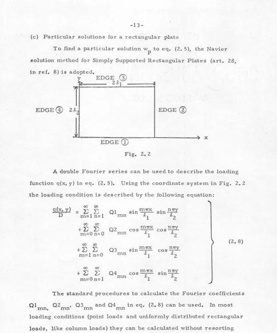
-13-(c) Particular solutions for a rectangular plate

To find a particular solution w to eq. (2. 5), the Navier

. p

solution m ethod for Simply Supported Rectangular Plates (art. 28,

in ref. 8) is adopted.

y EDGE

G)

'"l- 2.2.1

,.

EDGE@ EDGE@

~~---~---~---~' X

EDGE

CD

Fig.

2.

2

A

double Fourier series can be used to describe the loading function q(x, y) in eq. (2. 5). Using the coordinate system in Fig. 2. 2

the

loading condition is described by the following equation:

.six, y) D

00 6o

;;::

E

6

m=l n=l 00 00

+

ll

!)

m=O n=O

00 00

+

L) L)

m=l n=O

00 00

Ql s t n - -. mnx mn _.2.1 Q2

mn

mnx c o s

-t l

Q3 Sln-. mnx ~ -mn XJl

sin

..!!.!!.Y

.2.2 cos n'lry

.2.2

+

~ I; Q4 cos ~nx sin

!!..!!Y.

m=On:;l mn 1 .2.2

(2. 8)

The etg.ndard procedures to calculate the Fourier coefficients

01..-v>

_

n

I

en

1 Q3 and Q4 in eq. (2. 8) can be USed.

•• ~. mn tun mn In most

[image:17.570.14.561.28.687.2]

to numerical integration. However • for the most general loading

conditions, numerical integration is needed.

The particular solution

w

p

also can be expressed in double

Fourier series.

w = L)

:E

Bl s 1 n -. m'TTX - sin~

p

m=l n=l mn .R,l 1,2

+:E

I; B2 c o s - -m'!TX cos~

m=On=O mn .R,l 1,2

(2. 9)

+~

:E

B3 sin -m'!TX - cos !!.!!Y.

· m=l n=O mn .R,l 1,2

+:6 :E

B4 c o s -m'!TX - s1n . nny .R,

m=On=l mn .R,l 2

Substituting eq. (2. 9) and (2. 8) in (2. 5). each of the Fourier

coefficients should be equated. The Fourier coefficients in eq. (2. 9)

can be calculated from the known Fourier coefficients in eq. (2. 8).

For the sake of clarity this is explicitly stated as follows:

QI

BI

=

mn

mn

(2. 1 0)

where I denotes 1, 2, 3 or 4 as in eq. (2. 9).

Several examples of particular soiutions have been worked

out in detail in Appendix D. They include:

(i) A point load inside the plate.

(ii) A point load on the corner of the plate

(iii) A point load on the edge of the plate.

(iv) A column load {uniformly distributed load over rectangular

-15-In (ii) and (iii) some manipulation is employed to arrive at

the correct answer.

Equation (2. 9) only expresses the displace1nent of the

par-ticular solution. Properties of engineering interest other than

dis-placement are: slope, moment and shear. Mathematical

expres-sions of these properties of the particular solution are given in

Appendix E. They are obtained by substituting wp (as expressed

in eq. (2. 9)) for w in eq. (2. 4).

Now, it is presumed that the particular solution has been

found satisfying the differential equation. However, this solution

generally does not meet the required boundary conditions and is

therefore not unique. (There are many solutions that will satisfy

eq. (2. 5) ). Thus, the complementary solution has to be evaluated

to give a total solution (eq. (2. 7) ), which will satisfy the differential

equation and the required boundary conditions. To arrive at the

necessary complementary solution, the Edge -Function Method

developed by Quinlan {25) can be used. Chapter 3 introduces this

concept and describes its application to the plate problem. Chapter

4 deals with the specific use obtained by applying the Edge-Function

method to the rectangular plate problem.

This Fourier series representation of loading function given

by eq. (2. 8) can be used to describe any number of point loads, or

distributed pres sure, or even a combination of both types of loads

CHAPTER III. EDGE FUNCTION METHOD

After studying the Edge-Function idea developed by Quinlan (ZS)

to solve some very general plane strain or plane stress problems, R. F. Scott suggested the possibility of using this method to

tackle the case of a slab on a Winkler Foundation loaded

perpen-dicular to its plane. This has been examined and the following

discussion describes the application of this method of solving the

plate problem.

Quinlan's Edge Function idea is that, since the governing

differential equation is isotropic, (see Fig. 3. 1), its expression

in terms of the x-y coordinate system is of the same form as that

in terms of the x. ', y.' system or x ', y ' system. Therefore, a

J J q q

solution of the homogeneous equation in any coordinate system

(e.g. x. ', y. ') is also a solution to the differential equation with

J J

respect to other systems (e.g. x ', y '), providing the appropriate

q q

change of variable is performed. (In this case, x. ' , y. ' to x 1 _{, y ' . )}

J J q q

Furthermore, since the equation is linear, the solutions with respect

to various coordinate systems can be superimposed and the final

solution will still satisfy the equation with respect to any coordinate

system. This superimposed solution can be chosen such that the

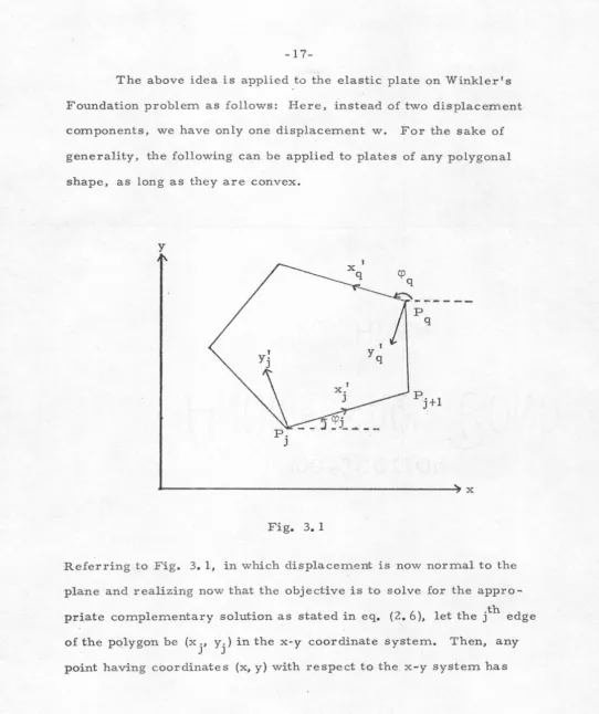
-17-The above idea is applied to the elastic plate on Winkler's

Foundation problem as follows: Here, instead of two displacement

components, we have only one displacement w. For the sake of

generality, the following can be applied to plates of any polygonal

shape, as long as they are convex.

y

p

q

~---~ x

Fig. 3. 1

Referring to Fig. 3. 1, in which displacement is now normal to the

plane and realizing now that the objective is to solve for the

appro-priate complementary solution as stated in eq. (2. 6 ), let the jth edge

of the pqlygon be (x j' yj) in the x-y coordinate system. Then, any

[image:21.575.18.560.33.679.2]

coordinates (xj', yj'} with respect to the xj', yj' system and the

coordinates are related to each other by the transformation shown

by eq. {3. 1 ).

x

=

x.

+

x. 1 _{co scp . - y.} 1 _{sincp .}

J J J J J

(3. 1)

y

=

y.

+

x. 1 _sincp.

+

_y. 1 _coscp.

J J J J J

The differential equation with respect to the (x, y) coordinate

system is given by eq. (2. 6). If another coordinate system (x 1_{, y ')}

is used, the differential equation has to be changed accordingly. To

find out what the differential equation will look like in the new system,

a coordinate transformation is performed on eq. (2. 6). From (3. 1)

a

ax

can be expressed in the xj1, yj' system.

a

ox

a

Similarly

oy

=

=

ox.'

oy.'

a

__j_

a

_:J__

ax.' ax

+

oy.'

ox

J J

a

coscpj

ax.'

J

.

a

s1ncp.

-J

ay.'

J

a

a

=

sincpj fu(."T

+

coscpj

ay.

1

J J

(3. 2)

Equation (3. 2) is applied successively in eq. (2. 6). Finally,

the transformed differ ential equation with respect to the new x 1 , y 1

system is

-::.4 j( I I) -::.4 j( I ' )

0 w X: ' Y· u w c X. ' Y· K .

+

2 c J J

+

---~J~-=J'--

+-

w J(x.', Y· ')

a

,2

a

,2

a

,4

o

c J J

xj , Yj Yj

-19-It can be observed that eq. (3. 3) is of the same form as

eq. (2. 6) if xj 1 _{and Yj} 1 _{is substituted for x and y respectively. From}

physical reasoning, since the plate and springs are isotropic and

homogeneous, the differential equation must be the same with respect

to any coordinate axes.

Furthermore, a solution wj(x. 1

, y. '). after changing x. ', y. 1

c J J J J

into any cartesian coordinate system (e. g. x '• y 1_{) using the}

appro-q q

priate form of equation (3. 1 ), will also satisfy the differential equa

-tion with respe~t to the xq1

• Yq1 system.

In other words, wj(x-1_{, y .}1_{) will satisfy the following equation:}

c J J

4 .

a

wJ(X· I Y· ')

c J • J

a

4 w j ( X j • I Yj I) K .

+

c 4

+

D wJ(x.', y.')

ay

'

c J J

q

=

0 (3. 4)

if xj'. y j' is changed into xq'• y q' appropriately following equation

(3. 1 ).

Because of the above property and since the equation (2. 6)

is linear, solutions with respect to different coordinate axes can be

superimposed and the total solution will still satisfy the differential

equation with respect to any particular set of axis. Thus, a very

general form of solution to the complementary equation (2. 6) can be

obtained as follows:

N

w (x, y) =

:B

c _J= . 1

wj(x-1 _{y ·')}

c J , J (3. 5)

where (x.!, y!) are related to (x, y) through eq. (3. 3), and are called

J J .

So far. the form of the co~plementary solution is known from

eq. (3. 5) and (3. 3). However. there are still sets of constants in

the complementary solution which remain unestablished. Applying

the boundary conditions on each edge. these constants are

deter-mined. In Chapter 4. an example will be given and the

complemen-tary solution to a rectangular plate solved in detail.

Other research applying the Edge Function idea is given

-21-CHAPTER IV. EDGE FUNCTION METHOD FOR A RECTANGULAR PLATE ON WINKLER FOUNDATION

The following chapter deals with finding the complementary solution that will satisfy the proper boundary conditions to a problem of a rectangular plate on a Winkler Foundation. The differential equation for the homogeneous problem is, from Chapter II

4

\] w

c +K D w c = 0 (2. 6)

For all rotated and translated coordinate systems, it will have the same form, as discussed in Chapter 3. One has to obtain solutions that satisfy the differential equation (3. 3). Using the particular

solution obtained in Chapter 2, the boundary conditions which arise from the particular solution will be easily given as a Fourier series. Thus, it is convenient to use Fourier series (sine and cosine) in the complementary solutions as well. First, let

. co mlTX.1 wJ = ~ sin J

c m=l .tj

. co

fJ{y.')+~

m J m=O

mlTX.1

COS ----:.t.,-j-"-

g~

( Y j I) ( 4. 1)

Substituting equation (4. 1) into equation (3. 3) two differential equa-tions arise as follows:

4 . _{2 . " j (IV) +}

K f j

}

( ~) f J- 2(mTr) fJ +f ₀

.t. m .t. m m D m =

J J _{(4. 2)}

(mTr )4 j _{2 (m1r)2 j"+} j(IV) K .

- g -

t.

_{gm gm} + - g J = 0

t.

m D m

J J

There are four independent solutions for each of equations (4. 2): g j and f j can both be expressed as linear combinations of the

m m

.,. j y. 1

e m J sin 9 j y. '

m J

'Y j Y· 1

e m J cos 9 j y. 1

m J

-y

j y.l

e m J sin 9 j y. 1

m J

-y

j Y· I

e m J cos 9 j y .1

m J

·where 9 j and ')I j have to satisfy the following equation:

m m

. 2 . 2

(mTT) 2

(y~)

-

(9~

=

_{I. .} J

2(')1 j) ( 9 j)

=

J~

m m

'Y j y.l

One can neglect the part involving em J in the solution

for each Edge Function with respect to a particular coordinate

(4. 3)

(4. 4}

' ) l l y l

system (e. g. e m 1 (sin

9~

y

1•

+

cos

9~

y 1

1_{) with respect to the}

coordinate system (x₁1_{, y}

1'). as can be seen from the following

discussion. The Edge Function method is basically a method of

superposition. Each of the superimposed elements has some property

which is governed by the boundary conditions. Their presence in

the solution is to introduce the boundary conditions at each edge of

the plate. Each of these elements has a particular form and a

par-ticular position. The different coordinate axes are set up in such

a way that the bases (y ·1 _{= 0) are located along the edges of the}

. J .

plate. (e. g. for a rectangular plate, the coordinate axes are set

up as shown in Fig. 4. 2.) From Fig. 4. 1, one can see that the Edge

Function w ~(x

1

•. y

1

1

-23-conditions on edge

(D.

When yJ. ::= 0 is substituted into the solution, w c' (x

1•, y J.

=

0) should constitute that part of the solution that makes the general solution behave according to the prescribed boundary conditions on edge

(D.

The function wc'(x

1•, y1') should become smaller with distance from edge

Q)

(y

1• getting bigger). At a point infinitely far away from the edge, the contribution from w c'(x

1•, y1') to the general solution should be zero. In effect, one is looking at a semi-infinite strip. When y

1•

=

0 certain propertief! are prescribed y J y.'

and as y 1

1

- oo, .the solution- 0. So, obviously thee m J part of the solution should be omitted from each Edge Function. The same

con-side ration holds for all the edges.

INFINITE STRIP

yl'

=

0

ASE OF EDGE

CD

PLATE UNDER CONSIDERATION

X, X 1

1

y

II\

EDGE

G)

,

21,3 ....

L

·"

I

!\

/ ...

':'-y4 x3

j = 3

II

x

4

.. I;

y3

21,4 j=4 j = 2 _21-2 EDGE@

' " yl

X I

1'-2

j = 1

,I/ xl _' Y2 / 'It __.!\,

,.

21-1 .... ,

"

X

EDGE

CD

Fig. 4. 2

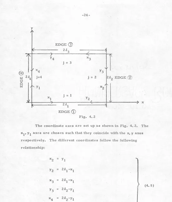
The coordinate axes are set up as shown in Fig. 4. 2. The

x

1• y 1 axes are chosen such that they coincide with the x, y axes

r espectively. The different coordinates follow the following

relationship:

x2 = yl

Y2 = 21-1-xl

x3 = 21-1-xl

y3 = 2 1,2-yl

x4

=

2 1,2-yl

Y4 = xl

[image:28.578.10.562.33.680.2]

-25-With the axes set up as shown in Fig. 4. 2, the most general

form of the complementary solution in the rectangular plate resting

on a Winkler Foundation is as follows:

where

4

00

=

~

:E

j=l m=l

4

00

+

6 6

j=l m=l

4

00

+

6

6

j=l m=O

4

00

+

6

6

j=l m=O

. m'!T"X. -y j Y· .

A J sin--,-"""- e m J sin 8 J y.

m f.. m J

J

- j

. m'!T"X. 'Y m YJ·

B J sin~ e

m

t.

J

. m 'IT"X.

-y

j y·.

C J cos~ e m J

m

t.

J

cos 8 j y·.

m J

sin 8 j y.

m J

. m '!T"X. -y y.

D J cos ___J_ e m J cos 8 j y.

m 1. m J

J

(yrl)2 - (8 j )2 ₌ (miT )2

m

t.

J

2(y j) (8 j ) ₌

J~

m m

In equation (4. 6) the only unknowns are the A j

m'

B

m' j

c

m j

(4. 6)

and D j • m

These coefficients are determined from the boundary conditions.

With these calculated, the exact complementary solution is known.

The particular solution is obtained from eq. (2. 9) and the total

solution can be calculated from eq. (2. 7 ). Mathematical

expres-sions of the complementary solution for slope, moment, and

shear force are given in Appendix E.

The remaining part of Chapter 4 will be used mainly to

illus-trate how the A j, B j, C j and D j are chosen so that the boundary

m m m m

Recalling eq. (2. 7), taking w _p to the left -hand side of the _. equation, the following is obtained:

. 4 .

wt(x, y) - w (x, y) = ~ wJ (x., Y;)

p j=l c J J (4. 7)

Changing coordinates of the above equation into any coordinate axes (e. g. x

1, y 1) and introducing the coordinate of that edge

Q) ,

the equation is reduced to that involving only one independent variable

(x

1, since y1 = 0 is the coordinate of edge

(D).

The following equa-tion is obtained:

4

=

~

w

1

(all coordinates changed to x 1)

j=l

(4. 8)

The function wt(x

1) in the above equation is the prescribed boundary

condition on edge(!). It can easily be represented by a Fourier

series. The displacement wp(x

1) is represented as a Fourier series

also. As a result the left -hand side is reduced to a single Fourier series. (A sine and a cosine series involving x

1). The right-hand

side of the equation, however, is more complicated. Referring to eq. (4. 6), after changing all the (xj, Yj) to (x

1, y1) and then after

substituting the coordinates of edge

Q)

(y

1

=

0), the following equation is obtained:

-2

7-00

w (on edge

Q)

)

=

c

6

1 . mmc1 oo 1 mmc1

B s1.n - - + 6 D cos

-m .tl m=O m .tl j=l

m=l

2 2

-y (2.t -x ) oo

2 -y (2.t -x )

m l 1 sin9 2(2.£1-xl)+ 6 D e m 1 1

00

+

6

c

2

m=O me m m=l m

cos 9

~

(2.t

1 -x1) j=2

-Y.3(2L) -/3(2L)

00 m TT'X]_ m ·-z oo ₃ m "TTXl m ·-z ₃

+6 A 3(-sin-.t-) sin9 3(2lz)+6 B (-sin-..e-) cos9 (21z)

m=l m 3 [e 3

~

m=l m 3(2: ) e Jm

oo mmcl 3 -yrJ2--z) 3 3 -ym 2 3

+ 6 cos

.t

C sin9~f2.t

2

)+D cos9 _{(2.t 2 )}

m=O ₃ m e ni m e m

j=3

4 co

+

6

m=O

-y X 00

4 m 1 . _{9 4} ""

Cm e Sl.n mXl + LJ

j=4

m=O

(4. 9)

In equation (4. 9) the part where j = 1 and j = 3 is a simple

Fourier series. However, when j = 2 and j = 4, the part involving

x

1 is not a Fourier series. In order to match the Fourier series,

on the left-hand side of eq. (4. 8), the part involving x

1 has to be

reduced to a Fourier series as well.

Letting

2

-y m (2 .tl -xl) 2 ~ . n"TTXl oo n"TTXl

e cos9m(2.t

1 -x1) = _{n=l n} LJ A s1.n-.t--₁ + 6 _n=O T] _n cos - n -_"'1

4

-y X

. 9 4 00 . nmc1 00 n"TTXl

m 1 _{6 6}

s

e s1.n m _{x 1} = _{pn s1.n}

-.t-

+ c o s

-n=l 1 n=O n .tl

4 -y X

4 00 nmc1 00 nmc1

m l

6 6 (4. 1 0)

e cos9mxl =

a

sin-..e- + w cos

~

n=l n 1 n=O n

where Tn' ~n' An' T]n' pn' r;n'

a

n

and

wn

are Fourie.r coefficients

.Substituting eq. (4. 1 0) into eq. (4. 9), the following equation m'TTXl ·m'TTXl

involving only sin and cos is obtained •

..e1 ..el

w (on edge

CD

).

c

oo

₁ . m'TTX₁

oo

₁ m'TTX = 2:; Bm Sl.n -..e-

+

2:; D cos 1

m=1 1 m=O m ..el

+

23

[23

c!J

Tm sin

~'TTX

1

+

23

I

23

c!]

13m cos -m--='TTX-1

m=l n=O 1 m=O Ln=O ..el

+

23

[-E

n

2

J

A sin

~'TTXl

+

I;

I

23

n

2

J

₁₁ cos

m=l n=O n m 1

m=OL~=O

n m

3

~ -ym (2 .t2)

+

2..j

-m=1 e

3 3 m'TTXl

sin 9 (2.t ) A sin

--:--==-m 2 m ..e

1

00

+

2:;

m=1

+

I;

-Y~

.

(

2

.t2) sine~

(2.t2)

c

3 cos m..e'TTX1

e m 1

m=O

Y

3(2.t ) 3 3 m'TTX1 ~ - m 2 cos 9 (2.t

2) D cos----.-::..

+

LJ e . m m

11

1

m=O

00

Goo

4

J

m'TTX1

+

2:; 2:; C p sin -..e-m=1 n=O n m 1

00

[00

4]

+

:6

:6

c

s

cos

m=O n=O n m

00

[00

J

+

6

6

D4 cr

m=1 n=O n m

oo

[

oo

4] m'TTX

+

:6

:6

Dn wm cos ..e 1

m=O n=O 1 ( 4. 11)

Equation (4. 11) is simply a Fourier series, in which the only unknowns are the A j B j C j and D j 1_{s. Equating this Fourier}

m' m' m m

series with that from the left-hand side of eq. (4. 8) (the coefficients

of the sine series with the sine series, and the coefficients of the

-29-linear equations in the unknowns A j 1 Bmj 1 C j and D j is

. rr1 m m

obtained.

For practical purposes, the index min eqs. (4. 9)1 (4. 10)1

and (4. 11) is truncated at m

=

N. Coefficients for m

>

N are neglected. So there are 4 X N A j 1 4 X N B j , and 4X (N+l)C j ,

m m m

and 4 X (N+l)D j• As a result there are 16N+8 unknown A j, B j,

m m m

C j and D j and the size of the matrix that has to be solved is

m m

(16N+8) by (16N+8). There are four edges and on each edge there

are two bounda_ry conditions. For each boundary condition there are N sine series and N+l cosine series coefficients. Therefore, there are 8 X (2N+l) equations that can be formed. Thus, there are

equal nmnbers of unknowns and equations and the matrix is well-defined. For boundary conditions other than displacements, the various deriv;;ttive of eqs. (2. 9) and (4. 6) have to be used. (See

eq. (2. 4) ). After solving for the A j, B j, C j and D j from the

m m m m

CHAPTER V. CONVERGENCE

The convergence of the solution by the Edge -Function method to the correct solution depends mainly on two conditions:

the smoothness of the prescribed boundary conditions and the

smoothness of the boundary condition contribution from the par-ticular solution. The parpar-ticular solution is given by a double sine, cosine series (eq. 2.9 ). After inserting the coordinates of the

edges in the particular solution, the function that describes the boundary contribution from the particular solution becomes simply a single sum Fourier series. Therefore, to simplify the problem, the Fourier transform of the prescribed boundary conditions from

the total solution (eq. 2. 7) is represented by a Fourier series

(a sine and a cosine). Thus, the convergence of the solution depends

mainly on the humber of terms required to represent adequately the particular solution as well as the prescribed boundary conditions.

The displacement in the particular solution is represented by eq. (2.

9).

On substituting the coordinates of the edges of the

plate into eq. (2. 9), w (x

* *

• y ). where (x ,

* *

y ) represents the

co-p

ordinates of an edge, the double sum series which originally has

two independent variables can be reduced to a single sum Fourier

series involving one independent variable if the coordinate system

with respect to that particular edge is used. To be more specific

-31-y

EDGE

Q)

.I ...

I

EDGE@)

2

~

yl EDGE@

II

xl

' X

'

2 .£,1

,

,_

EDGE

CD

Fig. 5.1

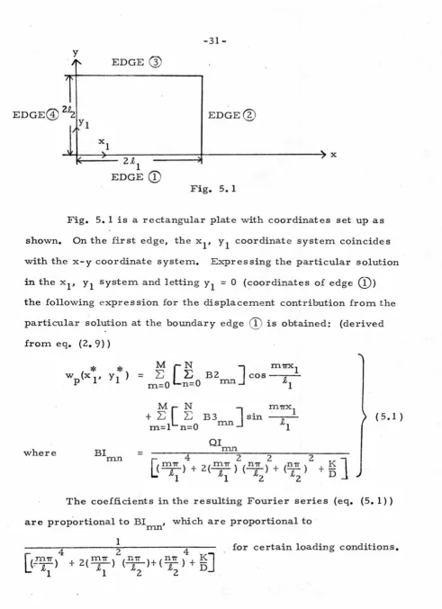
Fig. 5. 1 is a rectangular plate with coordinates set up as

shown. On the first edge, the x

1, y 1 coordinate system coincides

with the x-y coordinate system. Expressing the particular solution

in the xl' y₁ system and letting y₁ = 0 (c;:oordinates of edge

(D)

the following expression for the displacement contribution from the

particular solution at the boundary edge

Q)

is obtained: (derived

from eq. (2. 9))

where BI

mn

M [N

J

m'T!Xl

=

~

E

B2

cos--.--m=O n=O mn .£,1

( 5.1 )

=

The coefficients in the resulting Fourier series (eq. (5. 1))

are proportional to BI , which are proportional to mn

1

[image:35.570.45.536.38.715.2]

Thus, the particular solution for displacement on the boundary (Edge

Q)

in the example) converges like

_!_

4•

N

Similarly, using the slope equation for the particular solution in Appendix ~ the slope contribution of the particular solution on Edge

Q)

is given by the following:

*

y*)

a

w (x •

p on edge(!)

ayl

M [ N

1 .

n 'ITXl

"" "" B 1 ( n 'IT )

=

L.J L.J

J

Sl.n

-~--m=l n=l mn /-2 1

where the BI again behave like

~

•

mn

N

(5. 2)

The (¥_) factor which appears on differentiating the series

2

makes the coefficients in the Fourier series in eq. (5. 2) converge

slower and the slope in the particular solution converges as

~

• N

Similarly, (see eq. (1. 7)), we ca~ apply the same procedures to the moment and shear expressions in the particular solution given

in Appendix E. Since the moment basically involves the second

derivatives and the shear involves the third derivatives, the moment

1 1

converges as

z

and the shear converges as N N

To summarize: Displacement converges

1 Moment converges as _{N 2}

in the particular solution.

as 1

N4 Slope converges 1 Shear converges as N

as 1

-33;..

Thus. displacement converges very quickly. but convergence

is less rapid as higher derivatives are considered. In an actual

case, the double Fourier series have to be truncated at some term

N. Depending on the degree of accuracy desired and which

combi-nation of displacement slope. moment or shear is of interest, one

·can decide on where the series should be truncated. If the behavior

of the plate in terms of lower derivatives is desired, a smaller

number of terms is needed in the series.

The convergence of the complete solution, other than

depend-ing on the convergence of the particular solution, also depends to a

certain degree on the complementary solution. Referring back to

Chapter IV. on trying to choose the correct coefficients to use in

eq. (4. 6) such that the complementary solution w (x, y) will have the

c

desired value on the boundaries of the plate, eq. (4. 9) was derived.

This equation has to be matched with the left-hand side of eq. (4. 8)

which is given as a single sum Fourier series. If eq. (4. 9) is a

single sum Fourier series. the coefficients can simply be matched

term by term and the matrix is set up easily. However, eq. (4. 9)

is not a simple Fourier series, but involves some other functions.

That is why, in eq. (4. 9), the various functions have to be changed

to a Fourier series. These functions vary as the 9 j and y j which

m m

depend on the shape and dimension of the plate, soil spring constant

K and p!a.te constant D (the last two equations of eq. (4. 6) ). All of

these considerations will affect the smoothness of the various

functions in eq. (4. 9). Then, as these functions have to be

solution has to be large enough such that these functions can be

represented adequately in eq. (4. 10) by a Fourier series.

In general, it takes both a sine and a cosine series to expand

any general function. In solving the matrix, the Fourier coefficients

of all terms are coupled in each equation in the most general case.

Thus, if one wants to include terms as high as those involving

. N 'ITX N '7TX

s1n(-t-) and cos( ---:e-) terms, there are (16N+8) unknowns and

-35-CHAPTER VI. SYMMETRICAL PROPERTIES

In the course of this research, a computer program has

been set up to solve the rectangular plate problem; the matrix

that is solved in the program is arranged as shown in Fig. 6. 1.

As discussed in Chapter 5, in general a matrix of size

(16N+8) by (16N+8) has to be solved, N being the term where the

indices min the series given in eq. (4. 6) are terminated.

Symmetry in the problem of a thin plate on a Winkler

Foundation as solved by the Edge Function method is basically of

two types: (a) symmetrical boundary conditions, (b) symmetrical

boundary and loading conditions. The remainder of this chapter

deals with the two types of symmetries and how they can be used

to reduce the computer time needed to solve the problems:

(a) Boundary condition symmetries:

The boundary. conditions can be of four types: prescribed

displacement, slope, moment or shear. Any two of the above can

be prescribed on each edge. However, if the same type of

proper-ties is prescribed on each edge (e. g. displacement and moment are

prescribed on all edges) the matrix that has to be solved can be

reduced to one-fourth the size. This reduction can be made later

i f different functions of the same property (e. g. displacement) are

prescribed on each edge. If the same type of boundary conditions

are prescribed on all edges, the matrix as arranged ~n Fig. 6. 2

will be cyclic. A cyclic matrix is one which has submatrices [AJ,

[B ]. [C] and [D

J

arranged cyclically in the original matrix [M] as

1st B.

c.

N EQ.

SIN

I

I

E. F.

CD

I

•

cos

I

I

'

t

A 1 ; B 1

1c

1

:D

1

m m . m 1. m

I ' ~'1 _T / '

N COE₁ N COE N+l I N+l

:

I

COE : COE

ED

CD

- - - -- -

-

-- -

--:----1---:---

• I

2nd B. C.

N EQ.

1 • I

:

I

I

.

-

.

I

~·-·r-·

t

I

...!..

.

-- · -- ·

.. SIN

J.

II\

ED.@,

G);~

@,

Analogous

to

CD

(6N EQ.)

1st B.

c.

N+lEQ.

I

I

I

I

I

I ED.

CD

---

-

- - - -1-

-I I I I

I I

I

'

'

t

I t

.

I

I

I

I I I I I I I

I

•

I

• I

- L

----I

-

1---•

I

I

t

I

•

I

I

E.

F

.

@,@,@

Analogous to

CD

'

12N + 6 COE

-

-

---.

- ·

_

_,_

1

2nd B. C.

GOS- .

~+.lEQ

•• - •

r--•-•1--•

I

_j_ . -.

.

J__..

_ , _ , _

·-·

ED

.

@,

Q)

@

,

Analogous

to

(D,

(6N+6EQ.)

I

;

• I I

I

I

I

I

I

l

Abbreviations: E. F. -Edge Function, E. D. -Edge,

B. C. - Boundary Condition, COE. - Coefficients

Fig. 6. 1

[image:40.578.9.561.24.682.2]

-37-From Fig. 6. 1 one can shift the equations and partition the matrix into the form shown in Fig. 6. 2;

1st EDGE 2nd EDGE 3rd EDGE 4th EDGE

A 1 B 1 C 1 D 1

Analogous Analogous Analogous

EDGE B. C. m m m m to 1st to 1st to 1st

1st SIN

CD

2nd SIN

All Al2 Al3 Al4

1st

cos

2nd

cos

1st SIN

.

2nd SIN

@

_1st

cos

A21 A22 A23 A24

2nd

cos

1st SIN

2nd SIN

Q)

_1st

cos

_{A31 A32 A33 A34}

2nd I

cos

1st SIN

2nd SIN

@

_1st

cos

A41 A42 A43 A44

2nd

cos

Fig. 6. 2

The big matrix can be partitioned into 16 submatrices. Each of the

submatrices is now (4N+2) by (4N+2) or one -fourth the size of the

[image:41.570.22.554.21.690.2]

A B

c

D

. [M]

=

D A B

c

c

D A B

B

c

D A

The original matrix that has been set up. If it is cyclic as shown

in the figure, computing time can be reduced.

Fig. 6. 3

Therefore, the following equation with unknown vector x has

to be solved.

[MJ

CeJ

=

(g} (6. 1)

Vector

E

is the right-hand vector and can be derived from the l

eft-hand side of eq. (4. 8) which is the known function describing the

reduced boundary condition which the complementary solution has

to satisfy on the boundaries.

If the matrix [M] in eq. (6. 1) is not cyclic, the original

matrix [M] of size 16N

+

8 by 16N

+

8 ha·s to be inv.erted. However,

when [M] is cyclic, the following can be done.

Suppose

[~J

=

_{(6. 2)} [image:42.573.16.569.33.681.2]

-39-and [M] in eq. (6. 1) is cyclic as shown in Fig. 6. 3, then the

following equation has to be solved.

[M] [~}

[

_B.

}

.j. _~ .j.

A B

c

D _{xl Rl}

D A B

c

_{xz Rz}

= (6. 4)

c

D A B _{x3 R3}

B

c

D A _{x4 R4}

A transformation matrix [S] can be chosen to transform

eq. (6. 4}. Pre -multiplying and pro -multiplying the cyclic matrix

[M] in eq. (6. 4) by [S] -l [S] (as shown in eq. 6. 4}, the equation

should still be the same since [S] -l [S] = [I],

S should be chosen such that SMS -l in equation (6. 5) is a

matrix where there are only non-zero elements along the diagonal

of the matrix. In other words

[E] 0 0 0

SMS-l = 0 [F] 0 0

[MD] = (6. 6)

0 0

[G]

0

0 0 0

[H]

where [E], [F], [G] and [H] are submatrices. L etting [MD] =SMS1

in eq. (6. 5) the following is obtained:

Thus =

s-

1 M -l

s

[g}

D

(6. 7)

Since MD is a matrix which has non-zero submatrices only

along the diagonal and each sub-matrix is only one -fourth the size

of the original matrix, the problem is reduced to just inverting four matrices each one -fourth the size of the original matrix. The cost of solving the matrix is proportional to N2 where N is the size of the matrix. Thus, the computer time is only one-fourth of the original in this cas e.

Now, the matrix S and S-l which diagonalizes [M] has to be

dis covered.

Let S be divided into 16 submatrices

soo SOl S02 S03

(S]

=

SIO s u s12 sl3

(6. 9)

s2o s21 s22 s23 s30 s31 s32 s 33

The sub matrix s

=

[I] 1 _exp (21Tmni_N )

rnn

.jN

(6.

1 0)

where i is an imaginary number. N is the number of submatrices

to a cycle, in this case, 4.

Thus, S

-1

=

[

I] _..!_

exp ( -21TNi mn )

mn

,;r:f

( 6. 11}

As indicated by the equation, the matrix S related to our problem

is

(S] -_- .!. ₂

[I] [I] [I] [I]

[I] i[I]

::-[

I] -i

[

I]

[I] - [I] [I] -[I]

[I]

-i

[

I] -[I]

i[I]

-41-[Ij

[I]

[I]

[I]

[S]-1 1

[I]

-i[I]

-[I]

i [I]

(6.

13)

=

2

[I]

-[I]

[I]

-[I]

[I]

[i]

-[I] -i

[I]

After performing the operation shown on eq. (6. 6) using (6. 12) and (6.13). the following is obtained (i being the imaginary number):

[A+B+C+D] 0 0 0

0 [A-C+iB-iD] 0 0

[MD]

=

(6.15)

0 0 [A-B+C-D] 0

0 0 0 [A-C-iB+iD]

From the notation used in eq. (6. 6)

[E]

=

[A] + [B] + [C] + [D]

[F] = [A] - [C] +i [B] -i [D]

(6.

14)

[G]

=

[A]

+

[C] - [B] - [D]

[H]

=

[A]- [C]-i [B]+i[D]

Since [MD] is a complex matrix, [MD] -l is complex also.

since [F] and [H] are complex, some manipulation is needed to

evaluate the inverse. The operation in inverting a complex matrix

is well-known.

Suppose [a +if3]-l

=

[P + i

Q]

J

Then [P]

=

[a+ f3 a-1 f3]-l

(6. 16)

and

[Q]

=

-

[a-l f3 P]

Thus, if one has to invert a complex matrix. (say [a+i f3]).

one has to evaluate [P] (the real part of the inverse) and then

[Q],

the imaginary part of the inverse) by eq. (6. 16 ).

From equation (6.15), [E]-l and [G]-l can be evaluated

easily since they are both real matrices. [F]-l and [H]-l can be

calculated using eq. (6. 1 6). To be more explicit let

a

=

[A]+ [C]

f3

=

[B] - [D]

[A]. [B]. [C]. [D]

being submatrices from the original matrix as

shown in Fig. 6. 3.

so.

= [a+if3]-l = [P+iQ]

and noting that from eq. (6. 15) the real part of [H] and [F] are the

same and their imaginary part are of opposite sign.

=

=

[P - i Q]

[P] and [Q] can be calculated from eq.

(6. 16).

[P]

[Q]

=

=

[ a+f3a -1

!3

r-1

-43-Thus, inversion of [F] and [H] is reduced (from above equation)

into calculating [a -l

J

and [a +

13

a -ll3] -l, both matrices being only one -fourth the size of the original matrix.

Since each inversion of matrix is only one -fourth of the

original size and there are four inversions, computer time in

in-verting the matrices is only one -fourth of that required to solve the

. original matrix.

After solving [MD] -l eq. (6. 8) can be applied to solve for [x}.

(b) Symmetry in boundary conditions as well as loading condition:

Other than the above -mentioned symmetrical properties .that

give rise to a cyclic matrix, another course of symmetry can arise

from boundary and loading conditions. If the prescribed boundary

conditions as well as loading conditions are symmetrical with respect

to all edges, then other than resulting in a cyclic matrix as

dis-cussed earlier in this chapter, the right-hand vectors

R.

1, ~

2

,

R.

3

and R

4 in eq. (6. 4) are identical to each other. So, obviously

~l,

_e

2, x3 and

,.e

4 must also be equal to each other. Letting

i

=

.,e

1

=

2£.2

=

~

3

=

~ and ~

=

~l

=

~

2

=

~

3

=

R4, then the following equation has to be solved

[[A]+ [B] +

[cJ

+

[nJ]

?k

=

R.

(6. 1 7)

Thus, all that needs to be done is to solve a matrix

[[A] + [B] + [C] + [D]

J,

which is one -fourth the original size and

CHAPTER VII. CONCLUSION AND EXAMPLES a) Conclusion ·

The previous chapters illustrate the application of the Edge

Function method on plate problems on a Winkler Foundation. A computer program has been set up such that it can be used to solve the problem of a thin rectangular plate on a Winkler Foundation. To

~tilize the program, the following has to be done:

1) Using numerical process or otherwise, evaluate the Fourier coefficients of the series expressing the loading conditions as discussed in Chapter II (b).

2) On each of the edges, evaluate the Fourier coefficients

of the series expressing the boundary conditions.

3) The Fourier coefficients evaluated in steps (I) and (2) are used as input data in the program already set up and the output will be the coefficients of Edge Functions on each edge (see eq. 4. 6 ).

Total solutions of displacements as well as slope, moment and shear

in both x and y directions at points shown in Fig. 7. I are also calcu-lated and presented as computer output.

The program can easily be modified for point loads and column loads such that step (1) can be incorporated into the main

program. The program can also be modified easily so that solutions

on any points in the plate can be calculated instead of following the

pattern shown in Fig. 7. I. A number of problems have been solved

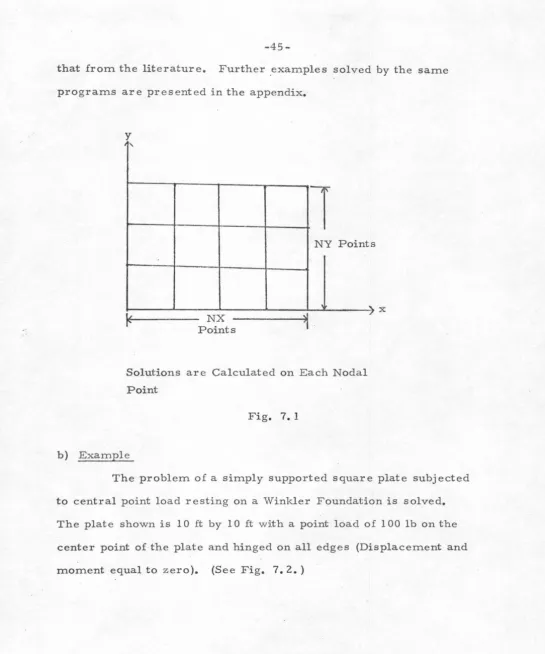
as examples. An example which has been solved using the computer

-45-that from the literature. Further _examples solved by the same

programs are presented in the appendix.

y

'

1

NY Points

NX

Points

Solutions are Calculated on Each Nodal

Point

Fig. 7.1

b) Example

'-/ X

The problem of a simply supported square plate subjected

to central point load resting on a Winkler Foundation is solved.

The plate shown is 10 ft by 10 fi with a point load of 100 lb on the

center point of the plate and hinged on all edges (Displacement and

[image:49.572.11.556.35.689.2]

/":'- Q

'I' R

- PLATE HINGED ON

ALL EDGES

0'

s

p S'

LOAD AT P

=

100 LB.

Q'

'

"

,

=

I

2.R,l 10

Solutions are Calculated at the Nodal Points

Fig. 7. 2

Solutions are calculated at the nodal points as shown. In

Tables 7. 5 and 7. 7, only those values at the nodal points in the

rec-tangular area PQRS are presented.

K

E

\)

h

D

p

The physical constants used in the problem are as follows:

spring constant of Winkler Foundation is 1 lb/£t3

Young's modulus for the elastic plate is 104 lb/£t2

Poisson's ratio ofthe plate is 0.2

. thickness of the plate is 0. 1 ft

Eh3 4

the plate constant given by ₂

=

0. 86805 £t

12(1-\1)

the characteristic length of the plate spring system is 4 ,.-rs-K _...J

K

=

o.

_{965 £t} [image:50.572.12.558.22.681.2]

-47-.t

1

i

length of the plate is 5 ft in the x-direction

.t

2

i

length of the plate is 5 ft in the y-dir ection

Tables 7. 1, 7. 3, 7. 5 and 7. 7 contain solutions calculated

from Timoshenko 1 _{s (}8_{) solution (chapter 8). Tables 7. 2, 7. 4, 7. 6}

and 7. 8 contain solutions calculated by the Edge Function method.

For equilibrium consideration for the Edge Function method

as well as the Timoshenko solution, the total upward force is

con-tributed from the spring force as well as the shearing force on the

boundary. The following table gives the values of the upward force

calculated. They are supposed to be equal to 100 lb when the total

downward load is applied. The spring force was calculated from the

displacements of the plate at each point and the shearing force

cal-culated from the shearing force in the normal direction on each edge

obtained from the 3rd derivative of the displacement along the edge.

COMPARISON OF EQUILIBRIUM

Edge Function Timoshenko

1 _s

Solution

Force from springs 90. 5 lb 87. 5 lb

Shear force on the edges 2. 3 lb 1

o.

6 lb

Total upward force 92. 8 lb 98. 1 lb

\

From Tables 7. 1 and 7. 2 the values of displacement agree

very closely (the maximum deflection is 13. 368 in Timoshenko 1 _s

solution and 13. 384 in the Edge Function method; 3 significant

figure of accuracy is achieved with 20 terms}. The slope results

Tables 7. 5 to 7. 8, the moment from both solutions does not agree

so well and shearing forces differ even more. As higher degrees

of differentiation are considered, the results from the Edge Function

method diverge more from Timoshenko 1 _{s solution. This is because}

the convergence in the Edge Function method deteriorates. To get

a better solution more terms would have to be taken.

Solutions on axis SPS' (see Fig. 7. 2). a line on the

mid-plate, are given on Fig. 7. 3 through Fig. 7. 5. Shear on Q 'PQ,

a line on the mid-plate parallel to Y axis, is plotted and given on

Fig. 7. 6, as shear in the Y direction is calculated instead of shear

0

~ 15

d

Cl>

s

10 Cl>

() n!

P..s

Ill

...

t::l 0

4

3

2

1 CD

s:::

n!

e

0

Cl> p..

0 _-1

...-i (/)

-2

-3

-4

-49-I

x:xx .Ti.moshenko s solution

Edge F·.mction solution

Length of Plate= 10 ft.

'

.

Fig. 7. 3 Plotting of Displacement along li"n~ SPS in Fig. 7. 2

I

[image:53.576.5.562.30.678.2]

~

[image:54.571.9.564.18.679.2]

0

... _..., 30

I

Timoshenko s Soluti