Longitudinal Data Modeling Using Multiscale Autoregresive (MAR) Wavelet

www.ijiset.com

25

Longitudinal Data Modeling Using

Multiscale Autoregresive (MAR) Wavelet

SupartiP 1

P

, Rukun SantosoP 2

P

, Alan PrahutamaP 3

P

, SudargoP 4

P

1,2,3

P

Departement of Statistics, Faculty Science and Mathematics, Diponegoro University, Semarang, Indonesia PGRI University Semarang, Indonesia

Corresponding Author: [email protected]

Abstract

Longitudinal data is a combination of cross section and time series data, where the subjects are independent and the time of observation of each subject is dependent. The advantages of studies on longitudinal data are knowing individual changes and requiring less subjects because of repeated observations. Moreover, the estimation is more efficient because it is done together for all subjects and observations. Some nonparametric methods for modeling longitudinal data are kernel, spline, local polynomial, fourier and wavelet. The wavelet method was developed to overcome the fourier method which is not good in modeling non-stationary data. In wavelet, Discrete Wavelet Transform (DWT) method is used. But there are limitations in DWT, because it can only be used for data modeling with the number of N= 2P

J

P

with J is positive integer numbers. In addition, the number of coefficients in DWT experiencing shrinkage as the scale level increases. To overcome this problem, Maximal Overlap Discrete Wavelet Transform (MODWT) is used, which can be used for any amount of data and the number of constant coefficients is as much as the processed data. By using the MODWT coefficient as an independent variable, longitudinal data modeling will be carried out, which each subject refers to the Autoregresive (AR) model and the model is called the Multiscale Autoregresive (MAR) Model . MAR modeling of longitudinal data is then applied to the simulation data of 3 subjects. Modeling is performed by using Haar (D2) and Daubechies (D4) filters with MAR level and order are 4 and 2 respectively. The modeling generated the best model with the Haar filter because it produces a smaller residual standard error and a greater coefficient of determination (RP

2

P

).

Keywords : Longitudinal data, MAR model, residual standard error, determination coefficient.

1.

Introduction

66T

In the regression analysis there are two types of data namely time series data and cross section data. Time series data is data from a subject that is observed repeatedly over time. While the cross section data is data from several subjects which are only done one observation on each subject and are mutually independent. According to Weiss (2005), longitudinal data is a special form of data with repeated measurements. The combined time series and cross section data form longitudinal data (Wu and Zhang, 2006). Longitudinal data is data obtained from repeated observations of each subject at different time intervals. This data correlates to the same subject and is independent between different subjects. According to Wu and Zhang (2006), there are several advantages of a study of longitudinal data, including knowing individual changes, and requiring not too many subjects because of repeated observations. In addition, the estimation is more efficient because it can be done together on all subjects and all observations.

66T

Research on longitudinal data include Hu et al (2004) using kernels. Liang and Zeger (1986) with the General Linear Model. Ibrahim and Suliadi (2008) used Smoothing Spline for longitudinal data, and Suparti, et al (2016) used local polynomials with case study modeling in 7 inflation spending groups in Indonesia. The kernel, smoothing spline and local polynomial methods are part of the nonparametic method. Other nonparametric methods that can be used for modeling longitudinal data are the Fourier and wavelet methods.

66T

Fourier transform can detect interference, but fourier transformation has some limitations, which require stationary data in the average so that the trend must be removed first before using the fourier transformation (Popoola, 2007). In addition, the results of the analysis of the data can only provide information about frequencies. This causes fourier transforms cannot be used to analyze non-stationary data.

66T

26

wavelet transforms that can be used to analyze non-stationary data. Wavelet is a function that mathematically cuts data into different components and studies each component with the appropriate resolution on the scale.

66T

Wavelet transform is divided into two major parts, namely Continuous Wavelet Transform (CWT) and Discrete Wavelet Transform (DWT). In DWT it is assumed that the sample size N can be expressed as 2P

J

P

for a positive integer J. This results in not all data being processed using DWT. A new concept was developed in overcoming the limitations of DWT in the sample size, namely Maximal Overlap Discrete Wavelet Transform (MODWT). MODWT has the advantage that it can be used for any N sample size (Percival and Walden, 2000).

66T

In this paper a study of modeling of longitudinal data using wavelets by utilizing MODWT and applying them to data on 3 inflation sectors in Indonesia, namely (1). Foodstuffs group; (2). Processed foods, beverages, cigarettes and tobacco groups; (3). Clothing group. These three expenditure groups are cases of longitudinal data.

2.

Methodology of Research

66T

Compile a longitudinal data layout according to the research case study. Forming MAR modeling using MODWT with J = 4 and Aj = 2 and estimating the parameters66T. 66TApplying research data modeling to data on sectors / groups of Indonesian inflation expenditure using the Haar (D2) and Daubechies (D4) filter with the initial procedure to calculate the MODWT for data on 3 sectors of inflation spending in Indonesia. Next determine the MODWT coefficient for each inflation spending sector data as input for the independent variable in the multiple regression model. Then estimate the parameters and test the significance of the model formed and calculate the coefficient of determination of the residual error standard. Perform a comparison of MAR models with filters D2 and D4, then choose the best model based on residual error and R2 standards. All calculations use the R software.

3.

Results and discussion

3.1.

Model Multiscale Autoregressive (MAR)

66T

In general, Multiscale Autoregressive wavelet modeling is a modeling method using wavelet transforms, in this case using MODWT. With multiscale decomposition like wavelet, there is a benefit that is obtained automatically separating data components, such as trend components and irregular components in the data. Therefore, this method can be used to make predictions on stationary and non-stationary data (Suhartono, et al, 2010).

66T

Suppose there is a stationary signal 𝑋= (𝑋₁, 𝑋₂, … ,𝑋_𝑡) 66Tand it is assumed to be a predicted value𝑋𝑡+1. 66TThe basic idea used is to use the coefficients obtained from the MODWT decomposition results 𝑤_{𝑗,𝑡−2}𝑗_(𝑘−1)and 𝑣_{𝐽,𝑡−2}𝐽_(𝑘−1), with 𝑘= 1,2, … ,𝐴_𝑗 and 𝑗= 1,2, … ,𝐽(Renaud et al, 2003). Predicted model follow the Autoregressive model (AR (p)), is 𝑋�_𝑡+1=∑𝑝_𝑘=1𝜙�_𝑘𝑋_{𝑡−(𝑘−1)}.

Replaced the independent variables XRtR, XRt-1R,... XRt-(p-1)R with coefficient from wavelet decomposition, Renaud et

al. (2003) given predicted model AR become Autoregressive (MAR) model:

𝑋�𝑡+1=∑𝐽_𝑗=1∑𝐴𝑘=1𝑗 𝑎�𝑗,𝑘𝑤𝑗,𝑡−2𝑗(𝑘−1)+∑𝐴𝑘=1𝑗 𝑎�𝐽+1,𝑘𝑣𝐽,𝑡−2𝐽_(𝑘−1) (2) with 𝑎_𝑗,𝑘 is coefficient MAR (j=1,2,...,J and k=1,2,...,𝐴_𝑗) and 𝐴_𝑗 is orde of MAR model, 𝑤_𝑗,𝑡 is coefficient of wavelet from the data, and 𝑣_𝑗,𝑡 is scale coefficient from data.

Figure 1 shows that wavelet (2) model formation in level J=4, 𝐴_𝑗= 2. It is illustrated that to predict the 18-th data with MAR (2) then input variables are coefficient wavelet 1-st level in t=17 and t=15, coefficient wavelet 2-nd level in t=17 and t=13, coefficient wavelet 3-rd level in t=17 and t=9, coefficient wavelet 4-th level in t=17 and t=1, coefficient scale 4-th level in t=17 and t=1.

66T

The MAR model has a shape similar to the multiple regression model, equation (2) can be written as:

𝑋𝑡+1=∑𝐽_𝑗=1∑𝑘=1𝐴𝑗 𝑎𝑗,𝑘𝑤𝑗,𝑡−2𝑗(𝑘−1)+∑𝑘=1𝐴𝑗 𝑎𝐽+1𝑘,𝑣𝐽,𝑡−2𝐽_(𝑘−1)+𝜀_𝑡+1 (3) For example, the number of data N=70, J=4 and A_j=2 (𝑘= 1,2), MAR model can be written as:

𝑋𝑡+1=� � 𝑎𝑗,𝑘 2

𝑘=1

𝑤_{𝑗,𝑡−2}𝑗_(𝑘−1)+� 𝑎_𝐽+1𝑘,

2

𝑘=1

𝑣_{𝐽,𝑡−2}𝐽_(𝑘−1)

4

𝑗=1

www.ijiset.com

27

𝑋𝑡+1=𝑎1,1𝑤1,𝑡+𝑎1,2𝑤1,𝑡−2+𝑎2,1𝑤2,𝑡+𝑎2,2𝑤2,𝑡−4+𝑎3,1𝑤3,𝑡+𝑎3,1𝑤3,𝑡−8+𝑎4,1𝑤4,𝑡+𝑎4,1𝑤4,𝑡−16+𝑎5,1𝑣4,𝑡

+𝑎5,2𝑣4,𝑡−16+𝜀𝑡+1

Signal

Level 1

Transformation Level 2

Wavelet Level 3 Level 4 Scale

t 1 2 3 4 5 6 7 8 9 10 11 12 13 14 15 16 17 18

Fig 2.

The

illustration of Wavelet Model for

J=4 and

𝐴

_𝑗

=2

Can be written as matrix:

⎣ ⎢ ⎢ ⎢ ⎢ ⎢ ⎢ ⎢ ⎢ ⎢ ⎢ ⎡𝑋_𝑋1₂

⋮ 𝑋16 𝑋17 𝑋18 𝑋19 ⋮ 𝑋𝑡 ⋮ 𝑋69

𝑋70⎦

⎥ ⎥ ⎥ ⎥ ⎥ ⎥ ⎥ ⎥ ⎥ ⎥ ⎤

=

⎣ ⎢ ⎢ ⎢ ⎢ ⎢ ⎢ ⎢ ⎢ ⎢ ⎢ ⎡ 𝑤_𝑤1₁,_,0₁

⋮ 𝑤1,15 𝑤1,16 𝑤1,17 𝑤1,18 ⋮ 𝑤1,𝑡−1

⋮ 𝑤1,68 𝑤1,69

𝑤1,−2 𝑤1,−1

⋮ 𝑤1,13 𝑤1,14 𝑤1,15 𝑤1,16 ⋮ 𝑤1,𝑡−3

⋮ 𝑤1,66 𝑤1,67

𝑤2,0 𝑤2,1 ⋮ 𝑤2,15 𝑤2,16 𝑤2,17 𝑤2,18 ⋮ 𝑤2,𝑡−1

⋮ 𝑤2,68 𝑤2,69

𝑤2,−4 𝑤2,−3

⋮ 𝑤2,11 𝑤2,12 𝑤2,13 𝑤2,14 ⋮ 𝑤2,𝑡−5

⋮ 𝑤2,64 𝑤2,65

𝑤3,0 𝑤3,1 ⋮ 𝑤3,15 𝑤3,16 𝑤3,17 𝑤3,18 ⋮ 𝑤3,𝑡−1

⋮ 𝑤3,68 𝑤3,69

𝑤3,−8 𝑤3,−7

⋮ 𝑤3,7 𝑤3,8 𝑤3,9 𝑤3,10

⋮ 𝑤3,𝑡−9

⋮ 𝑤3,60 𝑤3,61

𝑤4,0 𝑤4,1 ⋮ 𝑤4,15 𝑤4,16 𝑤4,17 𝑤4,18 ⋮ 𝑤4,𝑡−1

⋮ 𝑤4,68 𝑤4,69

𝑤4,−16 𝑤4,−15

⋮ 𝑤4,−1

𝑤4,0 𝑤4,1 𝑤4,2 ⋮ 𝑤4,𝑡−17

⋮ 𝑤4,52 𝑤4,53

𝑣4,0 𝑣4,1 ⋮ 𝑣4,15 𝑣4,16 𝑣4,17 𝑣4,18 ⋮ 𝑣4,𝑡−1

⋮ 𝑣4,68 𝑣4,69

𝑣4,−16 𝑣4,−15

⋮ 𝑣4,−1

𝑣4,0 𝑣4,1 𝑣4,2 ⋮ 𝑣4,𝑡−17

⋮ 𝑣4,52 𝑣4,53 ⎦

⎥ ⎥ ⎥ ⎥ ⎥ ⎥ ⎥ ⎥ ⎥ ⎥ ⎤ ⎣ ⎢ ⎢ ⎢ ⎢ ⎢ ⎢ ⎢ ⎢ ⎢ ⎡𝑎_𝑎1₁,_,1₂

𝑎2,1 𝑎2,2 𝑎3,1 𝑎3,2 ⋮ 𝑎𝑗,𝑘

⋮ 𝑎5,1 𝑎5,2⎦

⎥ ⎥ ⎥ ⎥ ⎥ ⎥ ⎥ ⎥ ⎥ ⎤

+

⎣

⎢

⎢

⎢

⎢

⎡

_𝜀

𝜀

1₂

⋮

𝜀

𝑡

⋮

𝜀

70

⎦

⎥

⎥

⎥

⎥

⎤

𝒔𝟏=𝐴1𝜶+𝜺𝟏 (4)

with:

𝐬𝟏 : vector of time series data with size 70 x 1; A1 : matrix of coefficient wavelet with size 70 x 10; 𝛂 : vector

of estimate parameter with size 10 x 1; 𝛆_𝟏 :vector error with size 70 x 1.

66T

The coefficients in matrix A, there are negative, zero and positive indexes. Coefficients with zero and negative indices are not found in the results of decomposition with wavelets. The formation of the MAR model is done by not including the coefficients of zero and negative indexes, so that the vectors s, ε and matrix A starting from the 18th row can be assumed as

𝐬= A𝛂+𝛆 (5)

𝐬 : vector of time series data with size 53 x 1

A : matrix of coefficient wavelet with size 53 x 10; 𝛂 : vector of estimate parameter with size 10 x 1 𝛆:

vector error with size 53 x 1

66T

As in multiple regression, to estimate the parameters in the MAR model can use the method of least squares (Ordinary least square), namely by minimizing the number of squares error:

∑ 𝛆ni=1 i2=𝛆T𝛆= (𝐬 −A𝛂)T(𝐬 −A𝛂) (6)

66T

By deriving the equation66T (6) to α then −2A

T_{𝐬+ 2A}T_{A𝛂= 0 ,so that can be obtained A}T_{A𝛂= A}T_{𝐬 or𝛂=}

(AT_A)−1_AT_{𝐬. So estimate parameter for model (5) is 𝛂�= (A}T_A)−1_AT_{𝐬 and 𝐬�= A𝛂�.}

66T

By using J = 4 and Aj = 2, there are 17 data that cannot be estimated using model (5), namely data 1 to 17. In its place, the authors estimate the data using the average data to 1-17.

66T

The longitudinal data that will be examined in this study is the longitudinal data with m subjects and observations of each subject are repeated n times. The data structure can be seen in Table 1

.

Table 1. Structure of Longitudinal Data

Subject Observation Dependent

1P

st

P

subject 1 XR1(1)

2 XR

2(1)

28

n XRn(1)

2P

nd

P

subject 1 XR1(2)

2 XR2(2)

 

n XRn(2)

  

m-th subject 1 XR1(m)

2 XR

2(m)

 

n XRn(m)

3.2.

MAR Model for Longitudinal Data

66T

The MAR model of the i-th observation subject to (t + 1) follows the following formula:

𝑋�𝑡+1(𝑖)=∑𝐽𝑗=1∑𝐴_𝑘=1𝑗 𝑎�𝑗,𝑘(𝑖)𝑤𝑗,𝑡−2𝑗(𝑘−1)(𝑖)+∑𝐴_𝑘=1𝑗 𝑎�𝐽+1,𝑘(𝑖)𝑣𝐽,𝑡−2𝐽(𝑘−1)(𝑖) (7)

with:

𝑎𝑗,𝑘(𝑖) : Coefficient of MAR i-th subject (j=1,2,...,J and k=1,2,...,𝐴𝑗and i =1,2,...,m ) 𝐴𝑗 : orde from MAR model

𝑤𝑗,𝑡(𝑖) : coefficient of wavelet level j-th from i-th subject in t-th observation

𝑣𝑗,𝑡(𝑖) : coefficient of scale level j-th from subject i-th in observation t-th.

66T

The selection of which wavelet coefficients are used to form the MAR Model (7), depends on the values of J and Aj. In this research, to build a prediction model at level J = 4, the order MAR A_j = 2 is used with j = 1,2,3,4. According to equation (7), the MAR model on the i subject becomes:

𝑋�𝑡+1(𝑖)=𝑎�1,1(𝑖)𝑤1,𝑡(𝑖)+𝑎�1,2(𝑖)𝑤1,𝑡−2(𝑖)+𝑎�2,1(𝑖)𝑤2,𝑡(𝑖)+𝑎�2,2(𝑖)𝑤2,𝑡−4(𝑖)+𝑎�3,1(𝑖)𝑤3,𝑡(𝑖)+ 𝑎�3,1(𝑖)𝑤3,𝑡−8(𝑖)+

𝑎�4,1(𝑖)𝑤4,𝑡(𝑖)+𝑎�4,1(𝑖)𝑤4,𝑡−16(𝑖)+𝑎�5,1(𝑖)𝑣4,𝑡(𝑖)+𝑎�5,2(𝑖)𝑣4,𝑡−16(𝑖) (8)

66T

By substituting variables from level 166T, 𝑤

1,𝑡(𝑖) = ZR1t(i)R, 𝑤

1,𝑡−2(𝑖) = ZR2t(i)R and coefficient 𝑎�

1,1(𝑖) = 𝛽̂1(𝑖), 𝑎�1,2(𝑖) =

𝛽̂2(𝑖). From level 2, 𝑤2,𝑡(𝑖) = ZR3t(i)R, 𝑤2,𝑡−4(𝑖) = ZR4t(i) Rand coefficient 𝑎�2,1(𝑖) = 𝛽̂3(𝑖), 𝑎�1,2(𝑖)= 𝛽̂4(𝑖). And so on, the last from level 4,𝑣_4,𝑡(𝑖) =ZR9t(i)R , 𝑣4,𝑡−16(𝑖) =ZR10t(i)R and coefficient 𝑎�5,1(𝑖) = 𝛽̂9(𝑖), 𝑎�5,2(𝑖) = 𝛽̂10(𝑖), then MAR model i-th subject as follow as:

𝑋�𝑡+1(𝑖) =𝛽̂1(𝑖) Z1t(i)+𝛽̂2(𝑖)Z2t(i)+𝛽̂3(𝑖)Z3t(i) +𝛽̂4(𝑖) Z4t(i)+𝛽̂5(𝑖) Z5t(i)+𝛽̂6(𝑖) Z6t(i)+𝛽̂7(𝑖) Z7t(i)+

𝛽̂8(𝑖) Z8t(i)+𝛽̂9(𝑖) Z9t(i)+𝛽̂10(𝑖) Z10t(i) (9)

66T

After removing the zero and negative indexes, there remains a positive index at t = 17.18, ..., N-1.

66T

In matrix, 66Tmodel (8) can be written as 𝐗�𝐭+𝟏(𝐢)=𝐙𝐭(𝐢)𝛃�(𝐢), i = 1, 2,..., m or: 𝐗�𝐭+𝟏(𝟏)=𝐙𝐭(𝟏)𝛃�(𝟏)

𝐗�𝐭+𝟏(𝟐)=𝐙𝐭(𝟐)𝛃�(𝟐)

⋮

𝐗�𝐭+𝟏(𝐦) =𝐙𝐭(𝐦)𝛃�(𝐦)

⎣ ⎢ ⎢ ⎢ ⎡𝐗�𝐭+𝟏(𝟏)

𝐗�𝐭+𝟏(𝟐)

⋮ 𝐗�𝐭+𝟏(𝐦)⎦⎥

⎥ ⎥ ⎤

= ⎣ ⎢ ⎢

⎡𝐙𝐭_𝟎(𝟏) _𝐙𝟎 … 𝟎 𝐭(𝟐) ⋯ 𝟎

⋮

𝟎 𝟎⋮ 𝟎 𝐙⋮ ⋮𝐭(𝐦)⎦

⎥ ⎥ ⎤

⎣ ⎢ ⎢ ⎢ ⎡𝛃�(𝟏)

𝛃�(𝟐)

⋮ 𝛃�(𝐦)⎦⎥

⎥ ⎥ ⎤

𝐗�𝐭+𝟏=𝐙𝐭𝛃�

𝛃� can be obtained from OLS with 𝛃� = (𝐙_𝐭𝑻𝐙_𝐭)−𝟏𝐙_𝐭𝑻𝐗_𝐭+𝟏 or𝛃�_𝐢= (𝐙_𝐭(𝐢)𝑻𝐙_𝐭(𝐢))−𝟏𝐙_𝐭(𝐢)𝑻𝐗_{𝐭+𝟏(𝐢)}

3.3.Case study

66T

The case study in this study is data on 3 sectors / groups of Indonesian yoy inflation spending from January 2007 to August 2017 taken from Bank Indonesia, namely (1). Foodstuffs group; (2). Processed foods, beverages, cigarettes and tobacco groups; (3). Clothing group. Descriptive statistics from data on 3 sectors of inflation expenditure in Indonesia are as follows

www.ijiset.com

29

Sector min max mean variance

Sector 1 1.452 20.020 8.810 18.63753 Sector 2 4.250 12.930 7.071 3.468268 Sector 3 -0.413 12.270 5.180 8.16835

66T

The first step is to decompose the MODWT of data on 3 groups of inflation spending in Indonesia using the Haar (D2) and Daubechies (D4) filters with a level (J) = 466T. 66TThe MODWT decomposition process will produce wavelet coefficients66T ( w ) and scale ( v ) that consist of wR1R, wR2R, wR3R, wR4R, and vR4R. Processing is done using software R. These coefficients will be used to form the MAR model input. The selection of wavelet coefficients used to form the Multiscale Autoregressive Model for each i-th sector follows the formula (8). 66TAfter getting the coefficients that will be used to form the model, continue modeling with OLS using R software for each subject.

3.4.Model Multiscale Autoregressive (MAR) withFilter Haar (D2)

66T

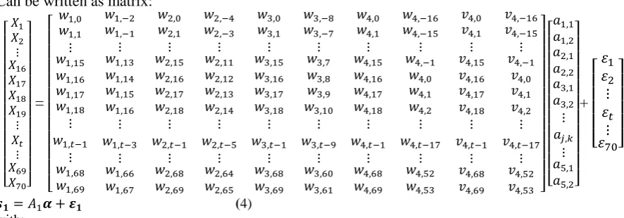
Sector 1 models are formed by entering ten independent variables66T ZR1(1)R, ZR2(1),R..., ZR10(1)R is : 𝑋�𝑡+1(1)= 1.86247 Z1𝑡(1)+ 0.23032 Z2𝑡(1)+ 0.43601 Z3𝑡(1)+ 0.38182 Z4𝑡(1)

+0.919 6 𝑍5𝑡−0.42526 Z6𝑡(1)+ 0.95677 Z7𝑡(1)−0.16585 Z8t(1)+ 0.95723 Z9𝑡(1)

+0.02208 Z10t(1)

66T

Together the model is significant with p-value < 2.2 x 10P

-16

P

, residual error standard of 1.269 and RP

2

P

of 0.983266T.

66T

The individually significant variable is the variable66T ZR1(1)R, ZR3(1)R, ZR5(1)R, ZR6(1)R, ZR7(1)R, ZR8(1)R and ZR9(1)R.

66T

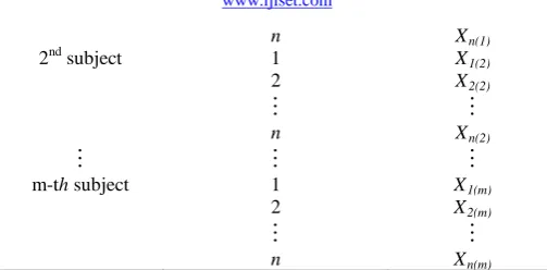
Sector 2 model formed by entering ten independent variables66T ZR1(2)R, ZR2(2),R..., ZR10(2)R are :

𝑋�𝑡+1(2)= 1.65308 Z1𝑡(2)+ 0.55415Z2𝑡(2)+ 0.49436 Z3𝑡(2)−0.22690Z4𝑡(2)+ 1.17423 𝑍5𝑡(2)

−0.36521 Z6𝑡(2)+ 0.99114 Z7𝑡(2)−0.18499Z8t(2)+ 1.07749 Z9𝑡(2)+−0.08326 Z10t(2)

66T

Simultaneous, the model is significant with p-value < 2.2x10P

-16

P

, residual error standard is 0.3806 and RP

2

P

is 0.9976. The individually significant variable is the variable66T ZR1(2)R, ZR2(2)R, ZR3(2)R, ZR5(2)R, ZR6(2)R, ZR7(2)R, ZR8(2)R , ZR9(2) Rand ZR10(2)R.

66T

Sector 3 model formed by entering ten independent variables66T ZR1(3)R, ZR2(3),R..., ZR10(3)R are :

𝑋�𝑡+1(3)= 1.40250 Z1𝑡(3)+ 0.56226 Z2𝑡(3)+ 0.45962 Z3𝑡(3)+0.10331 Z4𝑡(3)+ 0.53969 𝑍5𝑡(3)

− 0.35859 Z6𝑡(3) + 1.01910 Z7𝑡(3)−0.05276 Z8t(3)+ 0.99058 Z9𝑡(3)

−0.01733 Z10t(3)

66T

Simultaneous, the model is significant with p-value 66T

< 2.2x10

P

-16

P

,

66Tresidual error standard is 66T

0.9377 and R

P

2

P

sebesar 0.9741.

66TThe individually significant variable is the variable66T

Z

R1(3)R

, Z

R2(3) R

,Z

R3(4)R

, Z

R5(3)R

, Z

R6(3) R

, Z

R7(3)R

,

Z

R8(3)R

and Z

R9(3) R

.

66TGraphically the MAR model with the Haar (D2) filter formed in sectors 1-3 is presented in Figure 2-4.

Figure 2

. MAR Model with filter

D2 in Sector 1

Figure 3

. MAR Model with

filter D2 in sector 2

Figure 4

. MAR Model with filter

D2 in Sector 3

3.

5Model Multiscale Autoregressive (MAR) Filter D4

66T

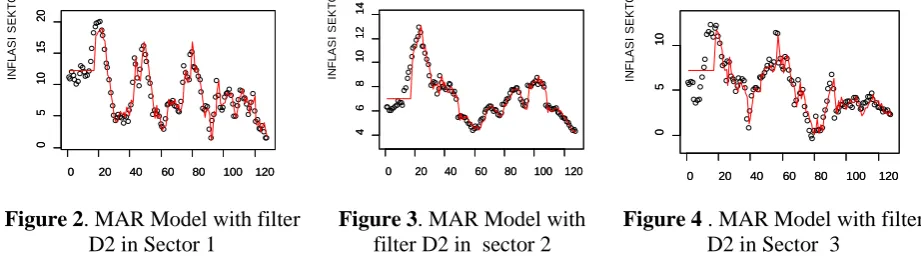
The MAR sector 1 model is formed by entering ten independent variables66T ZR1(1)R, ZR2(1),R..., ZR10(1) Ris : 𝑋�𝑡+1(1)= 0.21237 Z1𝑡(1)+ 0.55226Z2𝑡(1)+ 0.08748Z3𝑡(1)+ 0.13201Z4𝑡(1)−2.16025𝑍5𝑡(1)

−0.31032 Z6𝑡(1)−0.84086 Z7𝑡(1) −0.02900 Z8t(1)+ 0.57820Z9𝑡(1)+ 0.33102 Z10t(1)

66T

Simultaneously, the model is significant with a p-value < 2.210 x10P

-16

P

, a residual error standard of 3.4 and R2 of 0.879466T. 66TThe individually significant variable is the variable66T ZR5(1)R, ZR7(1)R, ZR9(1)R and ZR10(1)R.

66T

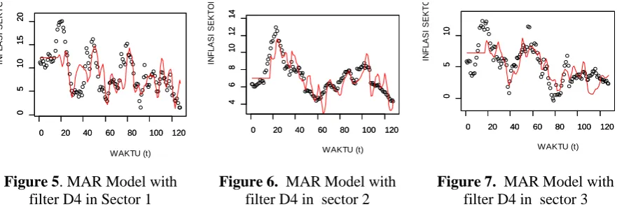
The MAR sector 2 model is formed by entering ten independent variables66T ZR1(2)R, ZR2(2),R..., ZR10(2)R is : 𝑋�𝑡+1(2)= 0.31058 Z1𝑡(2)+ 0.18636 Z2𝑡(2)−0.91212 Z3𝑡(2)+ 0.88090Z4𝑡(2) −4.15317 𝑍5𝑡(2)

−1.38979 Z6𝑡(2)−1.33224 Z7𝑡(2)− 0.34781Z8t(2)+ 1.24311 Z9𝑡(2)−0.27673 Z10t(2)

0 20 40 60 80 100 120

0

5

10

15

20

IN

F

L

ASI

SEKT

O

0 20 40 60 80 100 120

0

5

10

15

20

0 20 40 60 80 100 120

4

6

8

10

12

14

IN

F

L

ASI

SEKT

O

0 20 40 60 80 100 120

4

6

8

10

12

14

0 20 40 60 80 100 120

0

5

10

IN

F

L

ASI

SEKT

O

0 20 40 60 80 100 120

0

5

30

66T

Simultaneously, the model is significant with a p-value < 2.210 x10P

-16

P

, a residual error standard of 66T1.151 and RP

2

P

of 0.9776. 66TThe individually significant variable is the variable66T ZR5(2)R, ZR6(2), ZR R7(2)R, ZR9(2) Rand ZR10(2)R.

66T

The MAR sector 2 model is formed by entering ten independent variables66T ZR1(3)R, ZR2(3),R..., ZR10(3) Ris: 𝑋�𝑡+1(3)= 0.020490 Z1𝑡(3)− 0.002243Z2𝑡(3)+ 0.103098 Z3𝑡(3)+ 0.518868Z4𝑡(3)

−1.163302𝑍_5𝑡(3)−0.147765 Z_6𝑡(3)−1.125024Z_7𝑡(3)+ 0.783924Z_8t(3) + 0.838694Z_9𝑡(3)+ 0.059892Z_10t(3)

66T

Simultaneously, the model is significant with a p-value < 2.210 x10P

-16

P

, a residual error standard of 66T1.693 and RP

2

P

of 0.9156. 66TThe individually significant variable is the variable66T ZR5(3)R, ZR7(3)R , ZR8(3)R dan ZR9(3). R 66TGraphically the MAR model with the D4 filter formed in sectors 1-3 is as follows.

Figure 5

. MAR Model with

filter D4 in Sector 1

Figure 6.

MAR Model with

filter D4 in sector 2

Figure 7.

MAR Model with

filter D4 in sector 3

Table 3.66TComparison of MAR model results with Haar (D2) and Daubechies (D4) filters

Sector

Standar Error Residual

The number of Significant Coefficient

Coefficient of Determination (RP

2

P

)

MAR D2 MAR D4 MAR D2 MAR D4 MAR D2 MAR D4

1 1.269 3.4 7 4 0.9832 0.8794

2 0.3806 1.151 9 5 0.9976 0.9776

3 0.9377 1.693 8 5 0.9741 0.9156

66T

From the results of MAR modeling with Haar (D2) and Daubechies (D4) filters, it can be seen that the residual error standard for MAR models with filter D2 is always smaller than D4, the number of model coefficients is significant, MAR models with D2 tend to be more numerous than D4, and the magnitude of the coefficient of determination (R2) of the MAR model with filter D2 is greater than the model of MAR with filter D4. From Figure 2-4 and Figure 5-7, visually it can also be seen that the MAR model with the D2 filter is closer to the actual data. So the results of data modeling of 3 sectors / inflation expenditure in Indonesia using the Haar filter (D2) are better than the MAR model with filter D4. From the whole model formed using either the D2 or D4 filters the coefficients derived from the scale coefficient v4 are always significant. Because the scale coefficient provides the largest contribution to modeling.

4.Conclusion

66T

MAR modeling in data on 3 sectors of inflation expenditure in Indonesia using Haar filter (D2) both

statistically and visually shows better results than MAR models with Daubechies filter (D4)

Acknowledgment

66T

Thank you to Ministry of Research and Higher Education for funding this research with the PTUPT (Higher Education Applied Research) 2019.

Daftar Pustaka

0 20 40 60 80 100 120

0

5

10

15

20

WAKTU (t)

IN

F

L

ASI

SEKT

O

0 20 40 60 80 100 120

0

5

10

15

20

0 20 40 60 80 100 120

4

6

8

10

12

14

WAKTU (t)

IN

F

L

ASI

SEKT

O

R

0 20 40 60 80 100 120

4

6

8

10

12

14

0 20 40 60 80 100 120

0

5

10

WAKTU (t)

IN

F

L

ASI

SEKT

O

0 20 40 60 80 100 120

0

5

www.ijiset.com

31

[1] Hu Z, Wang N, dan Carroll RJ 2004 Profile Kernel Versus Backfitting In The Partially Linier Models

For Longitudinal Or Clustered Data Biometrika Vol 91 No 2 p 251-262

[2] Ibrahim NA dan Suliadi 2008 Analyzing Longitudinal Data Using Gee –Smoothing Spline Proceedings of the 8P

th

P

WSEAS International Conference on Applied Computer and Applied Computational science p 26-33

[3] Liang KY dan Zeger SL 1986 Longitudinal Data Using Generalized Linier Models. Biometrika Vol 78 No I p 13-22

[4] Percival DB danWalden AT 2000 Wavelets Methods for Time Series Analysis 1st Edn Cambridge University Press Cambridge p 620

[5] Popoola AO 2007 Fuzzy-Wavelet Method for Time Series Analysis (UK: University of Surrey)

[6] Renaud O, Starck J & Murtagh F 2003 Prediction based on a multiscale Decomposition. International Journal of Wavelets ( Multiresolution and Information Processing 1(2)) p 217-232

[7] Suhartono, Ulama BSS dan Endharta AJ 2010 Seasonal Time Series Data Forecasting by Using Neural Network Multiscale Autoregresive Model (American Journal of Applied Sciences 7 (10)) p 1373-1378 [8] Suparti, Prahutama A, Rahmawati R, dan Utami TW 2016 Modelling Local Polynomial for Longitudinal

Data A Case Study; Inflation sectors in Indonesia (ARPN Journal of Engineering and Aplied Science (JEAS) Vol 11 No 23)

[9] Weiss R E 2005 Modeling Longitudinal Data (New York: Springer)