R E S E A R C H
Open Access
Energy efficiency analysis of one-way and
two-way relay systems
Can Sun
*and Chenyang Yang
Abstract
Relaying is supposed to be a low energy consumption technique since the long distance transmission is divided into several short distance transmissions. When the power consumptions (PCs) other than that consumed by transmitting information bits is taken into account, however, relaying may not be energy efficient. In this article, we study the energy efficiencies (EEs) of one-way relay transmission (OWRT) and two-way relay transmission (TWRT) by comparing with direct transmission (DT). We consider a system where two source nodes transmit to each other with the assistance of a half-duplex amplify-and-forward relay node. We first find the maximum EEs of DT, OWRT, and TWRT by optimizing the transmission time and the transmit powers at each node. Then we compare the maximum EEs of the three strategies, and analyze the impact of circuit PCs and data amount. Analytical and simulation results show that relaying is not always more energy efficient than DT. Moreover, TWRT is not always more energy efficient than OWRT, despite that it is more spectral efficient. The EE of TWRT is higher than those of DT and OWRT in symmetric systems where the circuit PCs at each node are identical and the numbers of bits to be transmitted in two directions are equal. In asymmetric systems, however, OWRT may provide higher EE than TWRT when the numbers of bits in two directions differ significantly.
1 Introduction
Since the explosive growth of wireless services is sharply increasing their contributions to the carbon footprint and the operating costs, energy efficiency (EE) has drawn more and more attention recently as a new design goal for various wireless communication systems [1-3], compared with spectral efficiency (SE) that has been the design focus for decades.
A widely used performance metric for EE is the num-ber of transmitted bits per unit of energy. When only transmit power is taken into account, the EE monotoni-cally decreases with the increase of the SE [4] at least for point-to-point transmission in additive white Gaus-sian noise (AWGN) channel. In that case, when we minimize the transmit power, the EE will be maximized [5]. In practical systems, however, not only the power for transmitting information bits but also various signal-ing and circuits contribute to the system energy con-sumption (EC), which fundamentally change the relationship between the SE and EE. Specifically, when the circuit power consumption (PC) is considered, the
optimization problem that minimizes the overall trans-mit power does not necessarily lead to an energy effi-cient design [2].
Relaying is viewed as an energy saving technique because it can reduce the transmit power by breaking one long range transmission into several short range transmissions [3]. In fact, relaying has been extensively studied from another viewpoint, i.e., it is able to extend the coverage, enhance the reliability as well as the capa-city of wireless systems [6]. One-way relay transmission (OWRT) can reduce the one-hop communication dis-tance and provide spatial diversity, but its SE will also reduce to 1/2 of that of direct transmission (DT) when practical half-duplex relay is applied [7]. Fortunately, two-way relay transmission (TWRT) can recover the SE loss when properly designed [8-10]. However, it is not well-understood whether these relay strategies are energy efficient, when various energy costs in addition to transmit power are considered.
Considering both the transmit power and the receiver processing power, the EE of decode-and-forward (DF) OWRT systems was studied with single-antenna and multi-antenna nodes in [11,12], respectively. In [13], after accounting for the energy cost of acquiring channel * Correspondence: [email protected]
School of Electronics and Information Engineering, Beihang University, Beijing 100191, China
information, relay selection for an OWRT system with multiple DF relays was optimized to maximize the EE. In [14], the EE of DF OWRT was compared with that of DT, where the result shows that OWRT is more energy efficient when the distance between source and destina-tion is large, otherwise DT is better. In [15,16], the EEs of OWRT and base station cooperation transmission were compared, where the overall energy costs including those from manufacture and deployment were consid-ered. In [17], TWRT was shown to be more energy effi-cient than OWRT via simulations, where only transmit power was considered in the EC model. In [5], the EE of TWRT was compared with those of OWRT and DT, with optimized relay position and transmit power at each node. It shows that when the relay is placed at the midpoint of two source nodes, TWRT consumes less energy than OWRT and DT. Again, only transmit power was considered in the EC model. When we take into account the energy costs other than that contribu-ted by the transmit power, what is the results of com-parison between relaying and DT? Will TWRT still be more energy efficient than OWRT?
In this article, we analyze the EEs of TWRT, OWRT, and DT by studying a simple amplify-and-forward (AF) relay system. In literature, there are other relay proto-cols such as DF and compress-and-forward (CF) that provide higher rate regions than AF. However, AF is also widely considered in practice [6], and is superior to DF in outage performance for TWRT when the channel gains from two source nodes to the relay node are sym-metric [18]. Moreover, the system models differ a lot among the relay protocols. In order to analyze the maxi-mal EE, we need to find the relationship between end-to-end data rate and transmit power. With AF protocol, we can obtain the data rate-transmit power relationship by deriving the signal-to-noise ratio (SNR) at the desti-nation. With DF protocol, the end-to-end data rate is quite different, which is modeled as the lower one of the achievable data rates in two hops. When considering CF, the case is even more complicated since its trans-mission and processing procedure is usually very com-plex, which is rather involved for analysis. Here we focus on AF relay as a good start, while the EEs of other relay protocols will be considered in future studies.
We consider a delay-constrained system, whereBbits of message should be transmitted as a block within a duration T. This model is widely used for applications with strict delay constraints on data delivery, e.g., Voice-over-IP and sensor networks, where the message is gen-erated periodically and must be transmitted with a hard deadline [19-21]. Note that the energy consumed by transmitting information decreases as the transmission duration increases [4], but the energy consumed by cir-cuits increases with the duration. Therefore, in such a
system we can adjust the transmission duration to reduce the overall EC as long as the transmission dura-tion is shorter than the block length T. In other word, the system may transmit theBbits in a shorter duration than Tand then switch to an idle status until the next block [21]. During the idle status, a part of the transcei-ver hardware can be shut down, which can be exploited to improve the EE.
Specifically, we first maximize the EEs of TWRT, OWRT, and DT by optimizing transmission time and transmit powers, respectively, for the three strategies. We then compare the optimized EEs of TWRT with those of OWRT and DT. We show that when all the three strategies operate with optimized transmission time and power, relaying isnot always more energy
effi-cient than DT. Moreover, TWRT is not always more
energy efficient than OWRT if the numbers of bits to be transmitted in two directions are unequal, or the cir-cuit PCs at each node are different.
The rest of this article is organized as follows. System model and the ECs of the three transmit strategies are, respectively, described in Sections 2 and 3. Then the EEs of different strategies are optimized in Section 4. In Section 5, the optimized EEs are compared under varies circuit PCs and numbers of transmitted bits. Simulation results are given in Section 6. Section 7 concludes the article.
2 System model
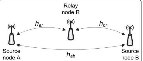
Consider a system consisting of two source nodes A and B, and an AF half-duplex relay node (RN) ℝ, each equipped with a single antenna. We consider a delay constrained system, where the information bits are gen-erated periodically and must be transmitted in a block within a hard deadlineT. In each block, nodesAandB, respectively, intends to transmit Bab andBba bits to each other with bandwidthW.In practice, the informa-tion bits to be transmitted in each block compose a packet or a frame, depending on application scenarios. In the following, we use the term“packet size” to refer the amount of data in each block, i.e.,Bab andBba.
The channels among three nodes are assumed as fre-quency-flat fading channels, which are respectively, denoted ashab, har, andhbr, as shown in Figure 1. We assume perfect channel knowledge at each node. The noise powerN0is assumed to be identical at each node.
Pci are, respectively, the circuit PCs in transmission, reception, and idle modes.
The circuit PCs inPctand Pcrconsist of two parts: the power consumed by baseband processing and radio fre-quency (RF) circuits. The PC of RF circuit is usually assumed independent of data rate [6,21], while there are different assumptions for the PC of baseband processing circuit. In systems with low complexity baseband pro-cessing, the baseband PC can be neglected compared with the RF PC [6,21]. Otherwise, the baseband PC is not negligible and increases with data rate [22]. In this article, we consider the first case, wherePctand Pcronly consist of RF PC, which are modeled as constants inde-pendent of data rate. ModelingPctandPcras functions of data rate leads to a different optimization problem, which will be considered in our future study.
The PC in idle modePciis modeled as a constant, and Pci≤ Pct, Pci ≤ Pcr. Subscripts (·)a, (·)b, and (·)r will be used to denote the PCs at different nodes.
3 Energy consumptions of three transmit strategies
We consider three transmit strategies, DT, OWRT, and TWRT, to complete the bidirectional communication between the two source nodes. In the following, we respectively introduce their ECs.
3.1 Direct transmission
In DT, nodes A and B transmit to each other without the assistance of RN. The transmission procedure is shown in Figure 2a. During each block, the system first allocates a durationTabfor the transmission from node
A to B, where node A is in transmit mode and node B is in receive mode. Then the system allocates a duration Tba for the transmission from node Bto A, where node
A is in receive mode and node B is in transmit mode. After the Bab andBbabits are transmitted, the system turns into idle status during T- Tab- Tba, where both nodes A and B are in idle mode. The EC of DT can be obtained as
ED=Tab(Pat/ε+Pcta +Pbcr) +Tba(Pbt/ε+Pctb +Pacr)
+ (T−Tab−Tba)(Pcia+Pcib)
=Tab(Pt
a/ε+PcD1+PDci) +Tba(Pbt/ε+PcD2−PciD) +TPciD (1)
where Pc1
D Pcta +Pbcr and PDc2Pbct+Pcra are,
respec-tively, the total circuit PCs in A→Band B→A trans-mission, and PciDPaci+Pcib is the total circuit PC in idle duration.
Given Taband Tba, nodes A and B should, respec-tively, transmit with data rates ofBab/Taband Bba/Tba bits-per-second (bps) to exchange theBabandBbabits messages, which are given by Shannon capacity formula as
Bab Tab
=Wlog2
1 +P
t a|hab|2
N0
, Bba
Tba =Wlog2
1 +P
t b|hab|2
N0
. (2)
Since Shannon capacity formula represents the maxi-mum achievable data rates under given transmit powers, the transmit power derived via this formula is the mini-mum transmit power that can support the required data rates. As a result, we can analyze the maximal EE for a given SE. We will also use the Shannon capacity formula to represent the relationship between data rates and transmit powers in OWRT and TWRT cases later. Figure 1A three nodes system. A three nodes system, where the
channels between Aand B, betweenA andℝ, and betweenB andℝare, respectively, denoted ashab,har, andhbr.
3.2 One-way relay transmission
In OWRT, each of the A→Band B→A transmission is divided into two hops, thus the bidirectional transmis-sion needs four phases, as shown in Figure 2b. For example, in A→B transmission, node A transmits to RN in the first phase, and RN transmits to node B in the second phase. With the AF relay protocol, the two phases in each direction employ identical time duration. For simplifying the analysis, we do not consider the direct link in OWRT. Although this will degrade the performance of OWRT, we will show later that it does not affect our comparison results for the EE.
The system allocates a durationTabfor A→B trans-mission. During the first half of Tab, node A transmits to RN, and thus node A is in transmit mode, nodeℝis in receive mode, and node B is idle. During the second half of Tab, RN forwards the information to node B, and thus node ℝ is in transmit mode, node B is in receive mode, and node A is idle. Then, the system allo-cates a duration Tbafor B→A transmission. Finally, the system turns into idle status duringT - Tab- Tba after the bidirectional transmission. The EC of OWRT can be obtained as
EO=Tab 2
Pt
a/ε+Pact+Prcr+Pcib+Prt1/ε+Pctr+Pcrb+Pcia
+Tba 2(P
t b/ε+P
ct b+P
cr
r +Paci+Ptr2/ε+Prct+Pacr+Pcib) + (T−Tab−Tba)(Pcia+Pbci+Pcir)
=Tab
Pt a+Ptr1
2ε +PcO1−PciO
+Tba
Pt b+P
t r2
2ε +PcO2−PciO
+TPci O,
(3)
where Prt1 and PTr2 are, respectively, the relay transmit
powers in A→B and B→A links,
POc1(Pct
a +Pcrr +Pcib +Pctr +Pcrb +Pcia)/2 and
Pc2
O (Pctb +Pcrr +Pcia +Pctr +Pcra +Pcib)/2 are, respectively,
the overall circuit PCs in A→B and B→A transmis-sion, and Pci
OPcia +Pcib +Prci is the overall circuit PC in
idle duration where all three nodes operate in idle mode.
The required bidirectional data rates can be obtained from the capacity formula and the expression of SNR for OWRT derived in [23], which are respectively,
Bab
Tab =
W
2 log2
1 + P
t aPrt1|har|
2|
hbr|2
|har|2Pt
aN0+|hbr|2Ptr1N0+N02
, (4)
Bba Tba
= W 2 log2
1 + P
t
bPrt2|hbr|2|har|2
|hbr|2PbtN0+|har|2Ptr2N0+N02
, (5)
where the factor 1/2 is due to the two-phase transmis-sion in each direction.
3.3 Two-way relay transmission
In TWRT, the bidirectional transmission is completed in two phases, as shown in Figure 2c. In the first phase, both nodes A and B transmit to RN, where the nodes
A and B are in transmit mode and the nodeℝ is in receive mode. In the second phase, RN broadcasts its received signal to the nodes A and B, where the node
ℝis in transmit mode, and the nodes A and B are in receive mode. After receiving the superimposed signal,
each of the source nodes A and B removes its own
transmitted signal via self-interference cancelation [8], and obtains its desired signal sent from the other source node. The two phases employ identical durations as in OWRT.
The system allocates duration TTWR to the
bidirec-tional transmission, and then turns into idle status dur-ingT-TTWR. The EC of TWRT is obtained as
ET=TTWR 2 (P
t
a/ε+Ptb/ε+Pcta+Pctb+Prcr) +
TTWR
2 (P t
r/ε+Pctr+Pcra +Pcrb) + (T−TTWR)(Pcia+Pbci+Pcir)
=TTWR
Pt a+Ptb+Ptr
2ε +P c T−PTci
+TPciT,
(6)
where PcT(Pact+Pctb +Pcrr +Pctr +Pcra +Pcrb)/2 and
PTciPci
a +Pcib +Prci are the overall circuit PCs in the
bidirectional transmission duration and the idle dura-tion, respectively.
The required bidirectional data rates can be obtained from the capacity formula and the SNR expression of TWRT derived in [23], which are respectively,
Bab
TTWR
=W 2log2
1 + P
t
aPrt|har|2|hbr|2
|har|2PtaN0+|hbr|2PbtN0+|hbr|2PtrN0+N20
, (7)
Bba
TTWR
=W 2log2
1 + P
t
bPrt|hbr|2|har|2
|har|2PtaN0+|hbr|2PbtN0+|har|2PtrN0+N20
, (8)
where the factor 1/2 is due to the two-phase
transmission.
4 Energy efficiency optimization for three transmit strategies
In this section, we optimize the EEs for DT, OWRT, and TWRT. The EE is defined as the number of bits transmitted in two directions per unit of energy, i.e.,
ηEE=
Bab+Bba
E , (9)
whereEis the EC per block, which respectively equals toED,EOorETin DT, OWRT, or TWRT.
sizes Bab and Bba. From the definition of hEE, we see
that EE maximization is equivalent to EC minimiza-tion for a given pair ofBab andBba. Consequently, we will minimize the EC per block for different strategies by optimizing transmission time and power of each node.
We consider that the transmission time should not exceed the duration of a block T, and the transmit power of each node should be less than the maximum transmit power Ptmax. Note that the system may not be able to transmitBabandBbabits within the durationT even if the maximum transmit power is used. In this case an outage occurs. Since we assume perfect channel knowledge at each node, the nodes can estimate the transmit power and the transmission time required for each block, which depend on the channel distribution and packet sizesBab andBba. Once the channel statistics and the packet sizes are given, the outage probability is fixed. In practice, the packet sizes Baband Bba can be pre-determined according to the quality of service (QoS) requirements, channel environment, and the acceptable outage probability. We will use Monte-Carlo simulation to find the maximalBabandBbathat ensure the outage probability to be lower than a threshold, e.g., 10%. Then, we only need to consider the EE optimization when the packet sizes are smaller than the maximum Baband Bba.
4.1 Direct transmission
As shown in (3), the EC of DT is a function of the transmit powers Pt
a and Pbt as well as the transmission
timeTabandTba. The EC can be minimized by jointly optimizing the transmit powers and transmission time as follows,
To solve this joint optimization problem, we first express the transmit powers Pt
a and Pbt as functions of
the transmission timeTaband Tba by using (2), which are respectively,
By substituting (11) into both the objective function and the constraints of (10), the problem (10) can be reformulated as follows,
The minimum value constraints on Taband Tbaare due to the transmit power constraints, without which the data rates Bab/Tab andBba/Tbawill be too high to be supported even with the maximal transmit powers.
Note that the problem in (12) is equivalent to the joint optimization problem in (10), where now only the transmission time needs to be optimized. In the objective function of the problem in (12), the first term is a function of Tab and not related toTba. It is easy to show that its second order derivative with respect to Tab is positive. Thus it is a convex function of Tab. Similarly, the second term in the objective function is a convex function of Tba. The last term is independent of the transmission time. Therefore, the objective function is convex with respect to Tab and Tba. All the constraints in (12) are also convex.a Then the problem can be solved by using efficient convex optimization techniques, such as gradient descent algo-rithm [24].
4.2 One-way relay transmission
Similar to the DT case, we first express the transmit powers as functions of the transmission time using (4) and (5). Then the joint optimization of transmit power and transmission time can be solved with two steps: first find the optimal transmit powers as functions of the transmission time, then optimize the transmission time to minimize the EC.
For a givenTab, both Pt
a and Pbt can be obtained from
(4), where multiple feasible solutions exist. In order to minimize the EC, we find the transmit powers that minimize the sum power as follows,
min
Pt a,Ptr1
Pta+Ptr1
s.t. Pta≤Pmaxt ,Ptr1≤Ptmax, and (4). (14)
Tab≥Bab/
Denote the minimum value of Pt
a+Prt1 as Pmin1(Tab),
where Tab ≥ Tmin1. It can be derived as a piecewise
function as follows (see Appendix 1),
Pmin 1(Tab) = Pmin1(Tab) follows (16), otherwise, it follows (17).
The piecewise function can be explained as follows. WhenTabis large, the data rate is low and both Pta and
Prt1 are below their maximum value, thenPmin1(Tab)
fol-lows the second part in (16) or (17). As Tabdecreases, one of Pt
a and Prt1 will achieve its maximum value.
When Tab= Td1, we have Prt1=Ptmax, and whenTab=
Td2, Pat =Ptmax. IfTd1 ≥ Td2, Ptr1 achieves its maximum
value first, Pmin1(Tab) follows the first part in (16).
Otherwise, Pt
a achieves its maximum value first, Pmin1
(Tab) follows the first part in (17). WhenTabdecreases toTmin1, both Pta and Prt1 achieve the maximum value.
For simplicity, we refer the first part in (16) or (17) as
“one-max” interval, because one of the nodes uses its maximum transmit power. We refer the second part in (16) or (17) as“non-max” interval, since neither of the nodes uses its maximum transmit power.
For a givenTba, we can also find the values of Ptb and
Pt
r2 that minimize their summation. Following an
analo-gous procedure, the minimum value of Pt
b+Ptr2 denoted
as Pmin2(Tba) can be derived as a piecewise function of
transmission timeTba, which are respectively,
Pmin 2(Tba) =
wise, it follows (19). The minimum value constraint for Tba, i.e.,Tba≥Tmin2, is also due to the maximum
trans-mit power constraint like that forTabin (15), and Tmin2
can be derived similarly asTmin1.
Then the optimization problem that minimizes the EC can be formulated as follows,
min
We can show that the first term in the objective function is a quasi-convex function ofTab(see Appendix 2). Simi-larly, the second term is a quasi-convex function ofTba. The last term is a constant. However, the sum of two quasi-convex functions may not be quasi-convex. There-fore, we solve this problem using the following approach.
First, we assume that the optimal solution for (20) satis-fies Tabopt+Toptba <T. In this case, the first constraint in (20) can be omitted. Since the second constraint is only related toTab, and the last constraint is only related to Tba, the joint optimization problem can be decoupled into two subproblems, i.e., optimizingTabto minimize the first term in objective function with the constraintTab≥Tmin1,
and optimizingTbato minimize the second term in objec-tive function with the constraintTba≥Tmin2. Because we
have proved that the first two terms in the objective func-tion are, respectively, quasi-convex funcfunc-tions with respect toTabandTba, both the two subproblems can be solved via quasi-convex optimization techniques such as bisection algorithm [24].
If the optimized Taband Tba from the two subpro-blems satisfy Tabopt+Tbaopt<T, then our assumption holds, and we obtain the optimal transmission time. Otherwise, the optimal solution for (20) must satisfy
Tabopt+Tbaopt=T. In this case, we only need to find the optimal Tabopt, where a scalar searching is applied, and
the optimal Tbaopt can be obtained as Toptba =T−Toptab .
4.3 Two-way relay transmission
Analogous to the previous sections, we first derive the transmit powers as functions of the transmission time.
For a givenTTWR, we can find Pta,Ptb, and P t
r from (7)
and (8), where multiple feasible solutions exist. To mini-mize the EC, again we find Pt
a,Pbt, and Prt that minimize
their summation from the following problem,
Following a similar derivation as in the case of
OWRT, the minimum value of Pt
a+Ptb+Prt can be
obtained as a piecewise function of the transmission timeTTWR, which is denoted asPmin(TTWR).
When TTWR is large, the data rates Bab/TTWR and Bba/TTWR are low, and all transmit powers are below
their maximum values. The optimal transmit powers are derived with similar method in Appendix 1 as follows,
Pta−opt=C1N0 |har|2
+ N0(C
2
1+C1+C1C2) |harhbr|
(C1+C2)(C1+C2+ 1) ,(22a)
Ptb−opt=C2N0 |hbr|2
+ N0(C
2
2+C2+C1C2) |harhbr|
(C1+C2)(C1+C2+ 1) ,(22b)
Ptr−opt=C1N0 |hbr|2
+C2N0 |har|2
+N0
(C1+C2)(C1+C2+ 1)
|harhbr|
.(22c)
where
C12
2Bab
WTTWR −1 and C22
2Bba
WTTWR −1.
The corresponding Pmin(TTWR) is the sum of (22a),
(22b), and (22c).
When TTWRdecreases, the data rates increases, then Pat−opt,Pbt−opt, and Ptr−opt increase until one of them
achieves the maximum value Pmaxt . By setting (22a), (22b), and (22c) to be Ptmax, respectively, we can obtain TTWR = Td1 when Pta−opt=Ptmax, TTWR = Td2 when Pbt−opt=Ptmax, and TTWR = Td3 when Prt−opt=Ptmax.
Without loss of generality, we assume that Td1 ≥ Td2
andTd1 ≥Td3(similar results can be obtained for other
cases). In this case, Pat−opt achieves the maximum value
first, i.e., node A transmits with the maximum transmit power. By substituting Pt
a=Ptmax into (7) and (8), we
have
Pat−opt=Ptmax, (23a)
Ptb−opt=C1C2N 2
0(|har|2− |hbr|2) +C2|har|2|hbr|2PtmaxN0 C1|har|2|hbr|2Pmaxt N0
,(23b)
Pt−opt
r =
C1C2N2
0(|har|2− |hbr|2) +PtmaxN0|har|2(C1|har|2+C2|hbr|2) +C1|har|2N20
|har|2|hbr|2(|har|2Ptmax−C1N0)
. (23c)
The corresponding Pmin(TTWR) can be obtained by
adding (23a), (23b), and (23c).
When TTWRfurther decreases, the data rates further
increases, Ptb−opt and Prt−opt in (23) increase until one of
them achieves its maximum value. Without loss of gen-erality, assume that Ptb−opt in (23b) achieves Ptmax first. The corresponding value of TTWRis denoted as Tmin,
which can be obtained by setting (23b) to be Pmaxt . Then both nodes A and Btransmit with the maximum power. Substituting Pt
a=Ptb=Pmaxt into (7) and (8), we
need to find one Pt
r from two equations, which has no
solution. Therefore,Tminis the minimum value ofTTWR
due to the maximum transmit power constraint. Finally, the minimal sum transmit power is obtained as
Pmin(TTWR) =
(23a) + (23b) + (23c),Tmin≤TTWR<Td1 (22a) + (22b) + (22c),TTWR≥Td1, (24)
where its first and second parts are, respectively, referred to as “one-max” and“non-max” interval for simplicity as that in the case of OWRT.
Then the optimization problem that minimizes the EC can be formulated as
min
TTWR
TTWR
Pmin(TTWR)
2ε +PcT−PciT
+TPciT
s.t.Tmin≤TTWR≤T.
(25)
Using the similar method in Appendix 2, we can prove that the objective function is a quasi-convex function of TTWR. Therefore, efficient quasi-convex optimization
tech-niques [24] can be applied to solve the problem.
5 Energy efficiency analysis
In this section, we compare the EEs of different transmit strategies, and analyze the impact of various channels and system settings.
From the objective functions in (20) and (25), we can see that the expressions of the ECs of OWRT and TWRT are quite complex because the minimal sum transmit powers are piecewise functions with very com-plicated expressions, i.e., (16), (17), (18), (19), and (24). To gain useful insight into the EE comparison, we con-sider the following two approximations.
Approximation 1: In the piecewise functions of Pmin1
(Tab), Pmin2(Tba), and Pmin(TTWR), we only consider the “non-max”interval, where none of the nodes achieves its maximum transmit power.
We take the functionPmin1(Tab) in (16) as an example
to explain the approximation. In the“non-max” interval, as transmission time Tab decreases, both transmit powers at nodes A and B, i.e., Pta and Ptr1, increase for supporting the increased data rateBab/Tab. In the “ one-max”interval, Pt
r1 has achieved its maximum value. As
Tab decreases, only Pt
a can increase to support the
increased data rate, thus Pt
a grows much faster than
that in“non-max”interval and approaches its maximum value rapidly. Therefore, the range (Tmin1,Td1) of the
Tabopt∈(Td1, +∞). Based on this observation, we only
consider the“non-max”interval in range (Td1, +∞).
Since we only consider the case where none of the nodes achieve its maximal transmit power, we do not need to consider the maximum transmit power con-straints. Therefore it is not necessary to consider the corresponding minimum value constraints on the trans-mission time in this section.
Approximation 2: In the expressions of Pmin1(Tab), Pmin2(Tba), and Pmin(TTWR), we respectively consider that
We take (26a) as an example to explain the approxi-mation, which affects the values of the transmit power Pmin1(Tab) and Pmin2(Tba) in OWRT. When the SEs in
two directions, i.e.,Bab/(WTab) andBba/(WTba) are high, it is easy to see that the approximations in (26a) are accurate. On the other hand, when the SEs are low, the transmit powers Pmin1(Tab) and Pmin2(Tba) are much
lower than the circuit PC. Then the approximations on transmit powers have little impact on the analysis of EC. By applying these approximations, the ECs of OWRT and TWRT can be simplified as
EO≈Tab
can be viewed as an
equivalent channel gain between two source nodes due to the usage of the relay.
For the convenience of comparison, we rewrite the EC of DT in the same form as follows,
ED=Tab
As a baseline for further analysis, we first consider the case where all the circuit PCs are zero and the packet sizes in two directions are symmetric, i.e., Pct=Pcr=Pci
= 0 and Bab=BbaB. Then the ECs of OWRT,
TWRT, and DT shown in (27), (28), and (29) are decreasing functions of the transmission time. As a result, the system will use the entire duration T for transmission. Due to the symmetric packet sizes, the optimal values ofTaband Tbaare identical in DT and OWRT. This means that the optimal transmission time in DT and OWRT are Tabopt=Tbaopt=T/2, and that in
TWRT is TTWRopt =T. After substituting the optimal transmission time into (27), (28), and (29), the minimum ECs can be obtained as
Emin
from which we can see that the optimal EE,
ηopt EE =
2B
Emin, is a decreasing function of the packet size
Bin the three strategies. This implies that the maximal EE is achieved whenBapproaches zero.
Now, we compare the EEs of the three strategies. First, it shows from (30) that Emin
O /EminT ≥1, which means
that TWRT is more energy efficient than OWRT. Second, we see that Emin
D /EminT =|heff|2/|hab|2, i.e., the
EE comparison between TWRT and DT depends on the effective channel gain |heff| and the direct link channel
gain |hab|. If |heff| > |hab|, TWRT is more energy
effi-cient, otherwise, DT is more energy efficient. To gain further insight into this comparison, we consider an AWGN channel,b where |hab|2 is normalized as 1, the distance from the RN to nodes A and B are,
respec-tively, d and 1 - d. Then |har|2=
, whereais the path loss attenuation
factor. Then the equivalent channel gain becomes
|heff|= 1/
which is related to the RN position. To maximize | heff|, the optimal relay position is the midpoint of the
two source nodes, i.e.,d= 0.5. In this case, |heff| = 2a/2/
2. Whena > 2, which is true in most practical channel environments, |heff| = 2a/2/2 > |hab| = 1, and TWRT is
Third, for DT and OWRT we have
traffic region, OWRT is more energy efficient. When
B→ ∞, 2
means that in high traffic region, DT is more energy effi-cient. An intuitive explanation is as follows. On one hand, OWRT needs two-phase for transmission in each direction, thus the data rate in each phase should be twice of that in DT, which requires more transmit power. On the other hand, OWRT has higher equivalent channel gain, which reduces the required transmit power. In low traffic region, doubling the lower data rate has little impact on the transmit power, and thus OWRT is more energy efficient due to higher equivalent channel gain.
Here we argue that even if OWRT exploits the direct link between A and Bfor spatial diversity, the conclu-sion will still be the same. With the direct link, the equivalent channel gain can be improved. However, the improvement is rather limited in most cases, because the signal attenuation between the two source nodes is much larger than that between the source nodes and the RN. Furthermore, OWRT has 1/2 spectral efficiency loss with respect to DT and TWRT, which cannot be recovered from the SNR gain.
5.2 Impact of circuit power consumption
In this subsection we assume symmetric packet size, i.e., Bab=Bba=B, but consider the non-zero circuit PCs in practical systems. Then the ECs in (27), (28), and (29) are no longer monotonically decreasing functions of the transmission time. With the increase of the transmission time, the transmit energy decreases since the required data rate reduces, however, the circuit energy increases linearly. We take TWRT as an example to analyze the EE.
The optimal transmission time in TWRT can be obtained by taking the derivative of ET in (28) with respect toTTWRand setting it to be zero, which is
dET
is the bidirectional SE of
TWRT.
Although it is difficult to obtain a closed form solu-tion of the optimal TTWR, some observations can be
obtained from (33). The optimal SE that minimizes the EC should satisfy (33c), from which we can see that
ηopt
EE−Tdoes not depend on the packet sizeB.Therefore,
the optimal transmission time TTWRopt =
2B
WηoptSE−T increases
linearly with B. Considering that TTWR should not
exceed the time duration of a block T, we obtain the following observation.
Observation 1:In high traffic region, ToptTWR=T. In low
traffic region where 2B
WηSEopt−T ≤T, the optimal
transmis-sion time TTWRopt =
2B
WηSEopt−T increases linearly with the
packet sizeB.
In high traffic region, the transmission time ToptTWR=T,
then the bidirectional SE2B
WT increases linearly with the
packet sizeB, thus the transmit energy increases expo-nentially with B according to the capacity formula. In this case, the transmit EC is much larger than the cir-cuit EC, thus the EE will be almost the same as that in zero circuit PC scenario.
In low traffic region, when the system transmits with
the optimal transmission time TTWRopt =
2B WηoptSE−T, the
ToptTWR ⎡ ⎢ ⎢ ⎢ ⎢ ⎣
N0(2
2B WToptTWR−1) ε|heff|2
+PcT−P ci T ⎤ ⎥ ⎥ ⎥ ⎥ ⎦=
2BN0 ε|heff|2W
(ln 2)2 2B WTTWRopt
= 2BN0
ε|heff|2W
(ln 2)2ηoptSE−T,
where the first equality comes from the fact that (33b) equals to zero, and the second equality comes from
TTWRopt = 2B
WηSEopt−T.
By substituting Bab =Bba =B and TTWR=ToptTWR into
the EC of TWRT in (28), and then substituting (34), the minimum EC of TWRT can be obtained as
EminT = 2BN0
ε|heff|2W
(ln 2)2ηoptSE−T+TPci
T, (34)
and the optimal EE of TWRT is given by
ηopt EE−T=
2B
2BN0
ε|heff|2W
(ln 2)2ηoptSE−T+TPci
T
,
(35)
from which we can obtain the following observation. Observation 2:In low traffic region, if the circuit PC
in idle mode Pci
T = 0, we have η
opt EE−T=
ε|heff|2W
N0(ln 2)2η
opt SE−T
.
Since we have shown that ηoptSE−T does not depend on the packet sizeB, ηoptEE−Talso does not change withBin this case. If PTci= 0, lim
B→0η
opt
EE−T= 0 since a large portion
of energy is consumed in the idle duration. Note that although lim
B→0η
opt
EE−T= 0 due to the non-zero
idle mode circuit PC, this observation does not mean that the idle duration is unnecessary. If the system transmits with the entire durationT, where T>TTWRopt , it can save the EC in idle mode, but it wastes more EC in transmission mode because it does not transmit with the optimal transmission time. Finally, more energy will be consumed and the EE will be reduced. We will show this impact later in simulations.
Observation 2 shows that if PciT = 0,ηoptEE−T does not change withBin low traffic region, where 2B
WηoptSE−T ≤T,
i.e., B≤TWηoptSE−T/2. In other words, EE is insensitive to the packet size when B∈(0,TWηoptSE - T/2). We can show that such a region becomes wider as the circuit power
Pc
T increases. By taking derivative with respect to PcT at
both side of (33c), we obtain
1−N0(ln 2)
2
ε|heff|2
2ηoptSE−Tηopt
SE−T
dηoptSE−T
dPc
T
= 0, (36)
from which we can see that
dηSEopt−T
dPcT =
ε|heff|2
N0(ln 2)22η
opt SE−Tηopt
SE−T
≥0, i.e., as the circuit
power Pc
T increases, ηoptSE−T increases, and then the
region (0,TWηSEopt−T/2) extends.
Following analogous procedure, we can obtain the same observations as in the Observations 1 and 2 for DT and OWRT. The optimal EEs of DT and OWRT in low traffic region can be obtained as
ηopt EE−D=
2B
BN0
ε|hab|2W(ln 2)(2 ηopt
SE−D1+ 2η opt
SE−D2) +TPci
D
, (37)
ηopt EE−O=
2B
BN0
ε|heff|2W
(ln 2)(2ηSEopt−O1+ 22η opt
SE−O2) +TPci
O
, (38)
where ηSEopt−D1 and ηoptSE−D2 are the optimal SEs in
A→B and B→A directions in DT, ηoptSE−O1 and ηopt
SE−O2 are those in OWRT, none of them depends on
the packet size B.We omit the detailed derivations for concise.
Since it is difficult to derive closed form expressions for the optimal transmission time and the optimal SEs, there are also no closed form expressions for the opti-mal EEs. We will use simulations to compare the EEs of DT, OWRT, and TWRT under non-zero circuit PCs.
5.3 Impact of unequal data amounts in two directions
In this section, we assume that the circuit PCs are identical at each node, and consider that the packet sizes in two directions differ. Define Bab = bBs and Bba = (1 -b)Bs, whereBs is the overall number of bits to be transmitted in two directions, and b is a factor to reflect the traffic asymmetry. We will show that
onceBs is given, the minimum ECs of DT and OWRT
Proposition 1. The minimum EC of OWRT does not depend onb.
Proof. Since, we assume Pc1
O =PcO2POc , the EC of
OWRT in (27) can be rewritten as
EO=Tab
To minimize the EC, the optimal transmit time should satisfy that (see Appendix 3),
βBs Tabopt =
(1−β)Bs
Tbaopt RO, (40)
i.e., the data rates on the two directions are identical, whereROis not a function ofb.Then the minimum EO can be obtained as follows by substituting (40) into (39),
Emin
This proposition is easy to understand intuitively. Because with the optimized transmission time, the OWRT system transmits with the same data rate on each direction, and each bit is transmitted with identical data rateROand thus with identical time duration 1/RO. Therefore, the energy consumed by each bit is identical no matter in which direction it is transmitted. Then the minimum EC only depends on the overall number of transmitted bitsBs.
The minimum EC of DT, Emin
D , can be obtained in a
similar way, which also does not depend on b. We do not show the results for concise.
Proposition 2.The minimum EC of TWRT is a function
ofb, and its minimum value is achieved whenb= 0.5.
Proof.The EC of TWRT in (28) can be rewritten as,
ET=TTWR
If the transmission time in two directions could be different,cthe EC becomes
ET1=TTWR1
Note that the only difference of ET and ET1 is the
transmission time in their first and second terms. With less constraints on the transmission time, the minimum value of ET1 achieved by optimizing TTWR1and TTWR2
is a lower bound of the minimum value of ET by
opti-mizing TTWR, i.e.,
Following the analogous procedure as we analyze the OWRT system, we can show that EminT1 is not a function ofb. Moreover, using similar method as in Appendix 3, we can prove that the optimal TTWR1 and TTWR2 that
minimize (43) satisfy βBs
ToptTWR1 =
(1−β)Bs
ToptTWR2 . It suggests
that only when b= 0.5, TTWR1opt =TTWR2opt . In this case, by
lower bound Emin
6 Simulation results
In this section, we evaluate the EEs of the three trans-mission strategies, DT, OWRT, and TWRT, and validate previous analysis via simulations.
Simulation parameter settings are summarized in Table 1, where we consider that three nodes are located on a straight line, and the RN is at the midpoint of two source nodes. In this case, the equivalent channel gain in relaying achieves the maximal value. The small scale fading channels are independent and identically distribu-ted (i.i.d.) Rayleigh block fading, which remain constant during one block but are independent from one block to another. All the results are averaged over 500 channel realizations.
The increase of distance D, noise power N0, and
attenuation factora all result in higher required trans-mit power. Since their impacts are similar, we only show the impact of a. Because the increase of block duration T is equivalent to a reduction of the trans-mitted bits number per unit of time, we setT as a con-stant and change the values ofBab andBba.
From [6,21], the circuit PCs in practical systems usually range from dozens to hundreds of mW. There-fore, we set the circuit PCs in this range in the simula-tions. The power amplifier efficiency e is set as 0.35 [21].
6.1 Baseline case
We first compare the EEs of different strategies in the baseline case where the circuit PCs are zero and the packet sizesBab =Bba.
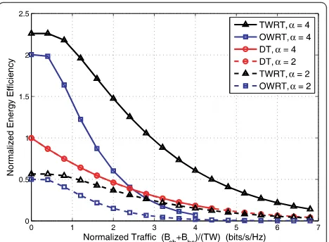
To show the EEs in different channel conditions, we set the attenuation factor a as 2 or 4. Since we are more interested in comparing the EEs rather than show-ing their absolute values, we normalize the EEs by the maximum EE of DT system for each a.The normalized EE is shown in Figure 3, and the corresponding outage
probability is shown in Figure 4. Thex-axis is the over-all number of transmitted bits in two directions normal-ized by the block duration and bandwidth, i.e., (Bab+ Bba)/(TW), which can be viewed as the average bidirec-tional SE per block.d
In Figure 3, because of the normalization, the EE curves of DT under different a overlap. It shows that the spectral efficient strategy TWRT is also energy effi-cient with respect to OWRT. When the attenuation fac-tor is large, i.e.,a = 4, the EE of TWRT is higher than that of DT, while when a = 2 the result is just the opposite. The comparison between DT and OWRT depends both on the packet size and the channel
condi-tion. When a = 2, DT always outperforms OWRT.
Table 1 List of important parameters
Symbol Definition Simulation setting
D Distance between source nodes Aand B 100 m
d, D-d Distance betweenA andBto relay nodeℝ 50 m
PL Path loss attenuation 30 + 10log10(distancea) dB
a Path loss attenuation factor 2, 4
N0 Noise power at each node -94 dBm
W Bandwidth 10MHz
T Block duration 5 ms
Bab, Bba Packet sizes in two directions ≥0
Power amplifier efficiency 0.35
Ptmax Maximum transmit power 40dBm
Pcta,Pctb,Prct Circuit power in transmit mode at each node From 0 to hundreds of mW Pcta,Pctb,Prct Circuit power in receive mode at each node From 0 to hundreds of mW Pct
a,Pctb,Prct Circuit power in idle mode at each node From 0 to hundreds of mW
Figure 3Energy efficiency comparison with zero circuit power and symmetric bidirectional packet sizes. Energy efficiency comparison with zero circuit power and symmetric bidirectional packet sizes. The curves of DT and OWRT witha= 4 respectively stop at (Bab+Bba)/(TW)= 4.4 and 4 bit/s/Hz, since larger packet
When a = 4, OWRT is superior to DT in low traffic region, but is inferior to DT in high traffic region. All these results agree well with our analysis.
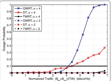
Figure 4 shows that whena= 2 the outage probabil-ities of DT, OWRT, and TWRT are zero for the consid-ered packet sizes. Whena = 4, the outage probabilities all increase. We see that TWRT offers lowest outage probability, and thus can support larger packet size given the same outage probability.
Since we only consider the case where the outage probability is lower than an acceptable threshold, say 10%, the EE curves of OWRT or DT whena = 4 is only plotted for the scenarios where (Bab + Bba)/(TW) is lower than 4 or 4.4 bits/s/Hz in Figure 3. In the follow-ing sections, we use the same method to determine the maximal packet sizes for DT, OWRT and TWRT, which ensure the outage probability to be lower than 10%.
6.2 Non-zero circuit power consumption
In Figure 5, we take TWRT as an example to show the impact of different circuit powers. We present the maxi-mal EEs, which are achieved by the optimized transmis-sion time and transmit power, i.e., there may be idle duration in each block. For comparison, we provide the baseline case again where the circuit PCs are zero. To show the necessity of the transmission time optimiza-tion, we also show the EE for a system who transmits with the entire block duration (i.e., there is no idle duration).
As expected, the non-zero circuit PC reduces the EE. It shows that the circuit PC only affects the EE in low traffic region, i.e., in low SE region. While in high SE region, since the transmit PC is much higher than the circuit PC, the EEs are almost the same for different
circuit PCs. That is to say, the high and low SE regions are, respectively,“transmit power dominant”and “circuit power dominant”.
When we assume the circuit PC in idle modePci= 0, i.e., there exists an idle duration but its PC can be ignored, the EE does not change with SE in the “circuit power dominant” region. As the circuit PCs in the transmit and receive modes Pct and Pcr increase, this region becomes wider.
WhenPci ≠0, the EE reduces to zero as the packet size decreases. Comparing the lowest two curves where Pci= 10 mW, we can see that the EE will decrease if we do not consider the idle duration, i.e., do not optimize the transmission time. Moreover, it is shown that when the PC in idle mode is not negligible, there is a non-zero optimal packet size that maximizes the maximal EE.
All these results agree with our earlier analytical ana-lysis. We do not show the results of OWRT and DT, which are similar as those of TWRT.
In Figure 6, we compare the EEs of different strategies with equal circuit PC at each node, where a = 4. It shows that the EE of TWRT is always higher than that of OWRT. Since the path loss is severe, TWRT outper-forms DT. OWRT is superior to DT in low traffic region, but becomes inferior in high traffic region. These results are the same as those in zero circuit PC scenario.
From Figure 6, we see that the idle mode circuit power Pci only affects the energy efficiencies in low Figure 4Outage probability with symmetric bidirectional
packet sizes. Outage probability with symmetric bidirectional packet sizes.
Figure 5 Energy efficiency of TWRT with different circuit powers. Energy efficiency of TWRT with different circuit powers: the attenuation factora= 4, circuit power consumptions at each node are identical, i.e.,Pct
a =Pbct=PrctPct,Pcra =Pcrb =PrcrPcr
traffic region, and the comparison result among differ-ent strategies will not change no matter Pci is zero or not. Since the different EE curves are more distinguish-able when the circuit power in idle mode is zero, in the following we set the circuit power in idle statusPci= 0
mW. Note that the circuit powers in transmit and receive modesPctandPcrare still non-zero.
In Figure 7, we compare the EEs with unequal circuit PCs at each node. We set the circuit PCs as
pctb =kbpcta,pcrb =kbpcra , where kb ≥ 1, which means that node B consumes more circuit power than node A. We also set pct
r =krpcta,pcrr =krpcra , where kr ≥ 1 or kr ≤ 1,
which reflects the cases where the RN consumes more circuit power or less circuit power than node A depend-ing on specific application scenarios.
It is easy to understand that if the circuit PC at the RN is high, the advantage of relay transmission over direct transmission shrinks and vice versa. Therefore, we focus on the comparison between OWRT and TWRT in Figure 7. We plot the performance gain of the maximal EE of TWRT over that of OWRT, i.e.,
max(ηoptEE−T) max(ηopt
EE−O)
, in order to observe whether TWRT is
more energy efficient than OWRT, and how much per-formance gain TWRT can achieve.
From the simulation results in Figure 7, we can see that askbincreases, i.e., the difference of the circuit PCs at the two source nodes becomes larger, the benefit of TWRT over OWRT shrinks. The OWRT even become more energy efficient than TWRT when the relay circuit PC is low.
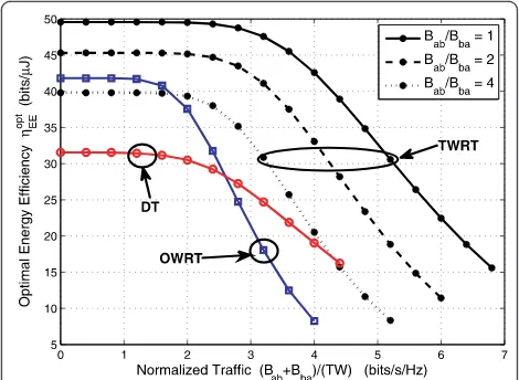
6.3 Unequal bidirectional packet sizes
Finally, we compare the maximal EEs with unequal bidirectional packet sizes, which are shown in Figure 8. It shows that the EEs of DT and OWRT do not depend on the ratio Bab/Bba, but the EE of TWRT reduces as Figure 6Energy efficiency comparison with identical circuit
power at each node. Energy efficiency comparison among TWRT, OWRT, and DT with identical circuit power at each node: the attenuation factora= 4, the circuit power consumptions are set as
Pcta =Pbct=Prct= 100mW,Pcra =Pbcr=Pcrr = 100mW, and
Pci
a =Pcib =Pcir = 0, 10 mW.
Figure 7 Performance gain of TWRT over OWRT in energy efficiency with unequal circuit powers at each node. The gain of the maximal energy efficiency of TWRT over that of OWRT, considering unequal circuit power consumptions at each node. The circuit powers of nodeA in transmit, receive, and idle modes are, respectively, Pcta = 50mW,Pcra = 100mW, andPci
a = 0mW.
The circuit powers of nodesBandℝare (Pctb,Pcrb,Pcib) =kb(Pct
a,Pacr,Pcia)and
(Pct
r,Pcrr,Pcir) =kr(Pcta,Pcra,Paci) wherekbandkrreflect the
unequal circuit powers at the three nodes. The attenuation factora =4.
Figure 8Impact of unequal bidirectional packet sizes. Impact of unequal bidirectional packet sizes: the attenuation factora= 4, circuit power consumptions
Pcta =Pbct=Prct= 100mW,Pcra =Pbcr=Pcrr = 100mW, and
the difference betweenBaband Bbaincreases, and may even become lower than those of OWRT and DT.
Note that in all the simulations, we did not consider the Approximations 1 and 2 employed in the beginning of Section 5. We can see that the analytical results using those approximations agree well with the simulation results. This validates the previous theoretical analysis.
7 Conclusion
In this article, we studied the energy efficiencies of OWRT and TWRT, and compared with direct transmis-sion. We first found the maximal energy efficiencies of three strategies by jointly optimizing the bidirectional transmission time and the transmit power. We then compared their maximal energy efficiencies with either zero or non-zero circuit power consumptions, and reveal the mechanisms to improve the energy efficiency of the three transmission strategies under different scenarios.
Analytical and simulation results showed that in sym-metric systems with equal circuit power at each node and equal packet sizes in two directions, the spectral efficient two-way relaying is also more energy efficient than one-way relaying, but two-way relaying only pro-vides higher energy efficiency than direct transmission when the path loss attenuation is large. In asymmetric systems where the circuit power consumptions at each node are different or the bidirectional packet sizes are unequal, the advantage of two-way relaying diminishes because it can not simultaneously minimize the energy consumed by the transmissions in two directions. One-way relaying may offer higher energy efficiency, depend-ing on the difference between the amount of data in two directions. Compared with the joint transmit power and transmission time optimization, only optimizing the transmit power has a loss in EE when the packet size is small. All the comparison results reveal that relaying is not always more energy efficient than direct transmis-sion, and the two-way relaying does not not always offer higher energy efficiency than one-way relaying. To save the energy consumption, a system should choose the most suitable transmission strategy considering its required amount of data to be transmitted, channel sta-tistics, hardware circuit powers, and so on.
We also showed the relationship between the energy efficiency and the spectral efficiency, i.e., the required amount of data normalized by bandwidth and time duration, for all the three transmission strategy, which is largely dependent on the circuit power consumption. With zero circuit power, the energy efficiency achieves its maximum value as the spectral efficiency approaches zero. With non-zero circuit powers in transmit and receive duration but negligible circuit powers in idle duration, energy efficiency does not change with spectral
efficiency in low traffic region but reduce sharply in high traffic region. With non-zero circuit powers in all the transmit, receive and idle modes, there exists a non-zero optimal spectral efficiency that maximizes the max-imal energy efficiency.
Appendix 1: Solution of optimization problem (14)
From (4), the transmit power at node A can be
expressed as a function of the transmit power at the RN in A→B link as
Pat = C1|hbr|
2Pt
r1N0+C1N20
|har|2|hbr|2Prt1−C1|har|2N0
f(Prt1), (44)
where C122Bab/(TabW)−1.
By substituting (44) into both the objective function and the constraints of (14), the optimization problem can be rewritten as
min
Pt r1
f(Prt1) +Prt1
s.t. f(Prt1)≤Pmaxt ,Ptr1≤Ptmax, (45)
which only depends on Pt r1.
It is easy to show that the objective function is convex by taking its second order derivative with respect to Pt
r1,
which is positive. Without the two constraints in this problem, the optimal Ptr1 can be obtained as follows by setting the first order derivative of the objective function with respect to Prt1 as zero,
Ptr−1opt= C1N0 |hbr|2 +
C2
1+C1N0
|harhbr| .
(46)
Then the corresponding optimal transmit power at node A can be obtained by substituting (46) into (44),
Pat−opt=f(Prt−1opt) =C1N0 |har|2 +
C21+C1N0
|harhbr|
. (47)
We can see that both Ptr−1opt and Pat−opt are increasing
functions of C1= 22Bab/(TabW)−1, thus are decreasing
functions of Tab. Therefore, whenTab is high enough, both Prt−1opt and Pat−opt=f(Ptr−1opt) will satisfy the two
constraints in (45). Then (46) and (47) are the optimal solutions of the problem (14).
As Tab decreases, both Prt−1opt and Pat−opt increase,
until one of them achieve its maximum value. By substi-tuting (46) and (47) into Prt−1opt =Pt
max and
demarcation point Tab =Td1 where Prt−1opt achieves its
maximal value, and can also derive the corresponding Tab=Td2where Pta−opt achieves its maximal value. The
imal value first, then we have
Prt−1opt=Ptmax. (50)
The corresponding Pta−opt can be obtained by
substi-tuting (50) into (44), which is
Pta−opt=
mal value first, then we have
Pat−opt=Ptmax. (52)
The corresponding Ptr−1opt can be derived using (44) by substituting (52),
(53), we can obtain the expressions of
Pmin 1(Tab) = min(Pta+Ptr1)in (16) and (17).
Appendix 2: Proof of quasi-convexity of the objective function in (20)
We consider the case that Pmin1(Tab) follows (16), the
conclusion is the same if it follows (17). Since Pmin1
(Tab) is a piecewise function of Tab,
is also a piecewise
func-tion. For simplicity, we define
Tab
By taking the second order derivative of fl(Tab), we have fl (Tab)≥0 when Tmin1 ≤ T <Td1. Therefore,fl
(Tab) is a convex function in the rangeTmin1≤T<Td1.
Then we will show thatfr(Tab) is a quasi-convex func-tion in the rangeT>Td1, where we will use the
follow-continuous on (xL, xR). Considering that
lim
with the assumption thatf”(x) only has one zero point. Assume thatf’(x) has two zero points such thatf’(a) =
two zero points for f”(x), which conflicts with the assumption thatf”(x) only has one zero point.
Consequently f’(x) can only has one zero point. Assume thatf’(xM) = 0. Then in (xL,xM),f(x) < 0, f(x) is non-increasing, while in (xM, xR),f’(x) > 0, f(x) is non-decreasing, which means that f(x) is a quasi-convex function in (xL,xR) [24].
By taking the derivative of fr(Tab), we find that
fr(0)→ −∞, and Tablim→∞fr(Tab) =POc1−PciO≥0 since
the circuit PC in the idle mode is lower than that in the transmit or receive mode. We also find that
fr (Tab) =k1[k2+k3g(Tab)], (55)
We can easily obtain that
lim
Tab→0
g(Tab) = 4, lim
Tab→+∞
Tab > 0. Theng(Tab) strictly monotonically decreases from 1 to -∞when Tab> 0. Therefore, f”(Tab) in (55) only has one zero point. According to Lemma 1,fr(Tab) is a quasi-convex function on (0, + ∞), and thus a quasi-convex function on [Td1, +∞).
Based on the expression ofTd1derived in Appendix 1,
we can obtain that Tlim ab→Td1
quasi-convexity of fr(Tab). Therefore,
Tab
Appendix 3: Derivation of the optimal transmission time
Recall that in Approximation 1, we only consider the case where none of the nodes achieves its maximal transmit power and thus we can ignore the minimum value constraints on transmission time. Then the opti-mization problem of the transmission time is given by
min
This is a convex problem, where the optimal Taband Tbashould satisfy the following Karush-Kuhn-Tucker (KKT) conditions,
wherelis the Lagrange multiplier.
We can see that the expressions in the left-hand side of (58b) and (58c) equal to each other. Therefore, the optimal transmission time satisfies
βBs Tabopt =
(1−β)Bs
Tbaopt RO. (59)
Substituting (59) into the KKT conditions, it is easy to see thatROis not a function ofb.
Endnotes
a
The feasible region of the EE optimization problem may be empty, which implies an outage of a block. Thereby we do not need to optimize for this block. Similar case also exists in the OWRT and TWRT opti-mization problems.
b
It should be noted that AWGN channel is appropri-ate for modeling free space propagation where a = 2. We consider different path loss attenuation factors here, which may be an abuse of the terminology of“AWGN channel”.
c
This can not happen in practice, which is considered only for the proof.
d
The average bidirectional SE per block takes into account the entire duration of a block, which includes not only the transmission time but also the idle duration.
Acknowledgements
We would like to thank Prof. Andreas F. Molisch and Prof. Zixiang Xiong for the helpful discussions. This study was supported in part by the National Natural Science Foundation of China (NSFC) under Grant 61120106002 and in part by National Basic Research Program of China, 973 Program 2012CB316003.
Competing interests
The authors declare that they have no competing interests.
Received: 29 September 2011 Accepted: 14 February 2012 Published: 14 February 2012
References
1. L Correia, D Zeller, O Blume, D Ferling, Y Jading, I Godor, G Auer, L Perre, Challenges and enabling technologies for energy aware mobile radio networks. IEEE Commun Mag.48(11), 66–72 (2010)
2. G Li, Z Xu, C Xiong, C Yang, S Zhang, Y Chen, S Xu, Energy-efficient wireless communications: tutorial, survey and open issues. IEEE Commun Mag.18(6), 28–35 (2011)
3. C Han, T Harrold, S Armour, I Krikidis, S Videv, PM Grant, H Haas, JS Thompson, I Ku, C Wang, T Le, MR Nakhai, J Zhang, L Hanzo, Green radio: radio techniques to enable energy-efficient wireless networks. IEEE Commun Mag.49(6), 46–54 (2011)
4. Y Chen, S Zhang, S Xu, G Li, Fundamental trade-offs on green wireless networks. IEEE Commun Mag.49(6), 30–37 (2011)
5. Y Li, X Zhang, M Peng, W Wang, Power provisioning and relay positioning for two-way relay channel with analog network coding. IEEE Signal Process Lett.18(9), 517–520 (2011)
6. M Dohler, Y Li,Cooperative Communications, Hardware, Channel & Phy, (Wiley, UK, 2010)
7. J Laneman, D Tse, G Wornell, Cooperative diversity in wireless networks: efficient protocols and outage behavior. IEEE Trans Inf Theory.50(12), 3062–3080 (2004). doi:10.1109/TIT.2004.838089
9. T Oechtering, E Jorswieck, R Wyrembelski, H Boche, On the optimal transmit strategy for the MIMO bidirectional broadcast channel. IEEE Trans Commun.57(12), 3817–3826 (2009)
10. C Sun, Y Li, B Vucetic, C Yang, Transceiver design for user multi-antenna two-way relay channels, inProceedings of IEEE Global Telecommunications Conference (GLOBECOM’10), Miami, Florida, USA, (December 2010), pp. 1–5
11. C Bae, W Stark, End-to-end energy-bandwidth tradeoff in multihop wireless networks. IEEE Trans Inf Theory.55(9), 4051–4066 (2009)
12. C Chen, W Stark, S Chen, Energy-bandwidth efficiency tradeoff in MIMO multi-hop wireless networks. IEEE J Select Areas Commun.29(8), 1537–1546 (2011)
13. R Madan, N Mehta, A Molisch, J Zhang, Energy-efficient cooperative relaying over fading channels with simple relay selection. IEEE Trans Wirel Commun.7(8), 3013–3025 (2008)
14. S Wang, J Nie, Energy efficiency optimization of cooperative communication in wireless sensor networks. EURASIP J Wirel Commun Netw.2010, 1–8 (2010)
15. D Cao, S Zhou, C Zhang, Z Niu, Energy saving performance comparison of coordinated multi-point transmission and wireless relaying, inProceedings of IEEE Global Telecommunications Conference (GLOBECOM’10), Miami, Florida, USA, (December 2010), pp. 1–5
16. P Rost, Opportunities, benefits, and constraints of relaying in mobile communication systems, (Technische University Dresden, 2009) PhD thesis 17. H Xu, B Li, XOR-assisted cooperative diversity in OFDMA wireless networks: Optimization framework and approximation algorithms, inProceedings of IEEE International Conference on Computer Communications (INFOCOM’09), Rio de Janeiro, Brazil, (April 2009), pp. 2141–2149
18. Q Li, S Ting, A Pandharipande, Y Han, Adaptive two-way relaying and outage analysis. IEEE Trans Wirel Commun.8(6), 3288–3299 (2009) 19. M Zafer, E Modiano, Optimal rate control for delay-constrained data
transmission over a wireless channel. IEEE Trans Inf Theory.54(9), 4020–4039 (2008)
20. J Lee, N Jindal, Energy-efficient scheduling of delay constrained traffic over fading channels. IEEE Trans Wirel Commun.8(4), 1866–1875 (2009) 21. S Cui, A Goldsmith, A Bahai, Energy-constrained modulation optimization.
IEEE Trans Wirel Commun.4(5), 2349–2360 (2005)
22. S Howard, C Schlegel, K Iniewski, Error control coding in low-power wireless sensor networks: when is ECC energy-efficient?. EURASIP J Wirel Commun Netw.2006, 1–14 (2006)
23. R Louie, Y Li, B Vucetic, Practical physical layer network coding for two-way relay channels: performance analysis and comparison. IEEE Trans Wirel Commun.9(2), 764–777 (2010)
24. S Boyd, L Vandenberghe, Convex Optimization, (Cambridge University Press, New York, 2004)
doi:10.1186/1687-1499-2012-46
Cite this article as:Sun and Yang:Energy efficiency analysis of one-way and two-way relay systems.EURASIP Journal on Wireless Communications and Networking20122012:46.
Submit your manuscript to a
journal and benefi t from:
7Convenient online submission
7 Rigorous peer review
7Immediate publication on acceptance
7 Open access: articles freely available online
7High visibility within the fi eld
7 Retaining the copyright to your article