DOA Estimation by Using Luneburg Lens Antenna with Mode
Extraction and Signal Processing Technique
Xiang Gu1, 2, *, Sidharath Jain3, Raj Mittra1, 4, and Yunhua Zhang2
Abstract—We propose a framework based on the use of a flat-base Luneburg lens antenna with a waveguide array for Direction-of-Arrival (DOA) estimation, and also present a hybrid approach which combines waveguide mode extraction and signal processing techniques for enhancing the angular resolution of the lens antenna. The hybrid method involves sampling the electric field at specified positions when the lens is operating in the receive mode, and extracting the weights of the possible propagating modes in each waveguide. Following this, we correlate these weights with the known ones that have been derived by either simulated or measured signals from single targets located at different look angles, to make an initial estimate of the angular regions of possible DOAs. We then apply an algorithm based on the Singular Value Decomposition (SVD) of the simulated or measured database to estimate the angles of incidence. Numerical results show that the proposed framework, used in conjunction with the hybrid approach, can achieve an enhanced resolution over the conventional limit base on the 3 dB beamwidth of the lens antenna. Furthermore, it is capable of locating targets with different scattering cross-sections and achieving an angular resolution as small as 2◦, for a Luneburg lens antenna with an aperture size of 6.35λand a Signal-to-Noise Ratio (SNR) of 30 dB.
1. INTRODUCTION
Wide-angle scanning and high angular resolution are highly desired in modern radar applications, for which the mechanically steerable antennas and phased arrays are currently employed [1]. However, antennas operated by a mechanical type of rotation device cannot meet the requirements of rapid beam-scanning and flexible control. Moreover, the phased arrays-although they are sophisticated and can serve multiple functions-are bulky, expensive to fabricate and often require complex hardware systems. The lens proposed by Luneburg [2] has the capability of all-angle-scan regardless of the operating frequency, as well as excellent focusing characteristics. Hence it is an attractive candidate for many scenarios calling for multi-beam, multi-frequency and multi-polarization scanning in 3D space. However, its gradient-index dielectric configuration is not only incompatible with the planar feeding and receiving devices, but it also poses some difficulties from fabrication point of view [3]. Recently, several research publications have focused on issues related to fabrication and realization of the Luneburg lens. They include the design and implementation of 2D/3D Luneburg lens antenna by using a Sievenpiper “mushroom” array [4]; a design based on liquid medium [5]; a parallel-plate waveguide with a Vivaldi antenna inside [6]; and air-filled parallel plates [7], just to name a few.
Other contributions have concentrated on the applications of the Luneburg lens antenna. The Luneburg lens was proposed as a potential antenna element for the Square Kilometer Array (SKA) radio telescope because of its multiple advantages of beam-forming, inherent wide bandwidth, and
Received 25 January 2015, Accepted 17 February 2015, Scheduled 18 March 2015
* Corresponding author: Xiang Gu ([email protected]).
very wide field of view [8]. Thanks to the recent technological advancements in realizing materials with desired electrical properties the Luneburg lens antenna can be fabricated at a relatively low cost, and it has attracted the attention of radar community. Specifically, Liang et al. [9] have fabricated a Luneburg lens antenna and have reported an approach for detecting a single source, by using five conformal detectors located on the curved surface of the lens. They have employed the Correlation Method (CM) [10] for the Direction-of-arrival (DOA) estimating in their work.
In this paper we propose a two-step approach consisting of waveguide mode decomposition followed by the use of a signal processing technique. The latter is a combination of the CM and the Singular Value Decomposition (SVD) algorithms to distinguish between different angles of arrival of the incident wave. To implement the proposed approach, a framework of Luneburg lens antenna with a waveguide array, which was initially proposed by Jain et al. [11] as a means to achieve wide angle scanning in the transmit mode, has been used. Numerical simulation results have verified the effectiveness and robustness of the two-step method.
2. LUNEBURG LENS ANTENNA WITH WAVEGUIDE ARRAY FOR DOA ESTIMATION
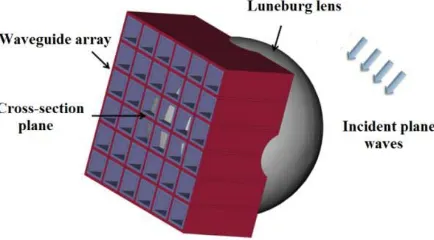
In [11], Jain et al. have proposed the design of a flat-base spherical Luneburg lens antenna which is fed by a planar waveguide array (see Figure 1). The Luneburg lens is designed to focus a plane wave, arriving from an arbitrary direction, at a point which is located diametrically opposite to that of the incident side. Luneburg has shown that the problem of findingεrof the lens can be formulated in terms of an integral equation [12], whose solution provides us the required material parameters of the lens. The radial variation ofεr is
εr = 2−(r/R)2 (1)
wherer is the distance from the center of the lens, and R is its radius.
Here, the same design has been used to develop a technique for DOA estimation because it not only preserves the salutary features of the conventional Luneburg lens, but is also much more convenient for measuring the fields on the planar surface of the array as opposed to the curved surface of the Luneburg lens. For instance, the waveguide array is not only highly efficient for extracting the signal from the incident waves in each waveguide, but it also has high isolation between the neighboring waveguides. This framework preserves the original properties of the Luneburg lens, namely wide bandwidth; wide scan angle capability and ability to handle multiple polarizations.
The spherical Luneburg lens (see in Figure 1) consists of 11 layers starting from the center. The first ten layers have a thickness of 3 mm each and the last layer is 1.75 mm thick. The dielectric parameters of the layers vary depending on their distance from the center [2]. The walls of the 6×6 waveguide array shown in Figure 1 are Perfect Electric Conductors (PECs) and they are 1 mm thick. Each waveguide has a square cross-section with a side length of 9 mm. It is well known that the angular resolution of an antenna is usually determined by the half-power beamwidth, which is inversely proportional to its aperture size. Assume that the aperture efficiency of the Luneburg lens is 100%, the predicted angular resolution is found to be 9◦, when the operating frequency is 30 GHz and the aperture sizeDis 63.5 mm.
3. WAVEGUIDE MODE EXTRACTION AND SIGNAL PROCESSING TECHNIQUES
To enhance the angular resolution of the lens, we propose a waveguide mode extraction technique followed by the use of a two-step signal processing algorithm. We begin by sampling the electric field at the cross-section plane of the waveguide array and then extracting the weights of the possible propagating modes in each waveguide. Next, we apply the correlation method to obtain an initial estimate of the possible DOAs. Following this we employ an SVD-based algorithm to achieve a more precise estimate of the DOAs.
Next, we detail the procedure for waveguide mode extraction. The cutoff frequencies of the electromagnetic waveguide can be complied from [13]:
fcutoff(m, n) =
1 2√με
m a 2 + n b 2 (2)
whereaandbrepresent the dimensions of the waveguide aperture at the transverse (x-y) plane;εandμ are the permittivity and permeability of the medium inside the waveguide, respectively; and the integers
m and nindicate different modes.
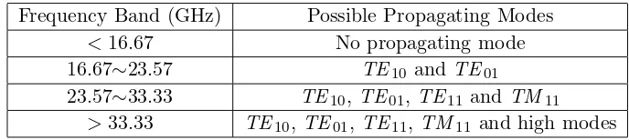
We set the operating frequency to be f = 30 GHz and choose the side dimensions of each square waveguide to be a = b = 9 mm. The cutoff frequencies for TE10, TE01, TE11 and TM11 modes are calculated using (2) and are found to be 16.67 GHz, 16.67 GHz, 23.57 GHz, and 23.57 GHz, respectively. The possible propagating modes within different frequency bands are listed in Table 1.
Table 1. Possible propagating modes within different frequency bands.
Frequency Band (GHz) Possible Propagating Modes
<16.67 No propagating mode
16.67∼23.57 TE10 and TE01
23.57∼33.33 TE10,TE01,TE11 and TM11
>33.33 TE10,TE01,TE11,TM11 and high modes
Once the possible modes are known, the field distribution on the face of each waveguide can be expressed as a weighted sum of the field distributions for these possible modes as follows:
˜
E=c1E˜TE10+c2E˜TE01+c3E˜TE11+c4E˜TM11 (3)
whereci (i= 1, 2, 3 and 4) are the weights of each mode andE˜TE10,E˜TE01,E˜TE11 and E˜TM11 are the bases corresponding to field distributions for TE10, TE01, TE11 and TM11 modes, respectively. The field distributions corresponding to the possible modes form a complete set of orthogonal bases; hence, they can be described any set of field distributions in the waveguide under consideration.
The weights can be obtained in two different ways. In the first approach, a dot product of (3) with the electric field distribution of the four modes is taken one at a time as follows:
˜ E·E˜
=c1
˜
ETE10 ·E˜
+c2
˜
ETE01·E˜
+c3
˜
ETE11·E˜
+c4
˜
ETM11·E˜
(4)
where E˜ representsE˜TE10,E˜TE01, E˜TE11 and E˜TM11. On doing so only one of the terms on the right hand side of (4) will be non-zero and hence the corresponding weight can be determined.
In the second approach, a matrixA, whose column comprises ofE-field components of four different modes, e.g., E˜TE10, E˜TE01, E˜TE11 and E˜TM11, is generated; hence we can relate the sampling data E˜ and the weights in matrix form as:
E=A·c (5)
Then using the inverse matrix operation, the weight of each mode is determined.
Ez-component, the maximum rank of A would be 2, 2 and 1, respectively. Hence, we should measure both Ex- and Ey-components to ensure that the matrix A is full-rank. Moreover, if all the sampling points are on a straight line, say along thex- or they-direction, the rank would again reduce to 3; and, hence, a unique solution cannot be obtained. To circumvent this problem, we employ four samples taken at differentx- andy-positions within the cross-section of the waveguides. Specifically, we set the sample points at (2.25 mm, 2.25 mm), (2.25 mm, 6.75 mm), (6.75 mm, 2.25 mm), and (6.75 mm, 6.75 mm) at the cross-section plane of each waveguide.
The step-by-step procedure can be summarized as follows:
(1) Measure the electric field distribution at the planar base of the Luneburg lens antenna with a waveguide array for different incident angles. Save the observed Ex-, and Ey-components of the field at the sampling points, and calculate the weights of the propagating modes in each of the 36 waveguides for each incident angle.
(2) Create a database matrix using the weights of the modes obtained in the previous step. The matrix consists of the weights of the modes in all of the waveguides for different angles of incidence. (3) Interpolate the database to achieve a finer interval for the angle of incidence. The finer database
matrix is written as B(N×M). Hence, we can generate an equation as follows:
eN×1=BN×M ·xM×1 (6)
whereB(N×M) represents the database, andN (i.e., 4×36 = 144) is the number of the weights and
M is the number of incident angles. Here e(N×1) represents the “measured” weights, andx(M×1) represents the possible DOAs.
(4) Calculate the weights of the modes from the “measured” data obtained from the field distribution due to unknown targets. Correlate the “measured” weights, i.e., e(N×1), to B(N×M) to determine the most probable target locations.
(5) Extract the columns of the database matrix that correspond to the most probable angular regions as a sub-database matrix, i.e., Bs(N×L), where L (L < M) represents the possible incident angles in the angular region of the initial estimate. Hence, (6) can be rewritten as:
eN×1 =BSN×L·xSL×1 (7)
where the matrixBs(N×L) corresponds to the most probable angular regions, andxs(M×1) represents the most probable regions of the DOA.
(6) Equation (7) usually represents an ill-posed problem. Hence, we apply the SVD to the sub-database matrix, i.e., to deriveBs=UDV, and use a threshold to reduce the matrix by deleting the singular vectors whose singular values fall below the threshold.
(7) Take a dot product of the K (K < L) remaining singular vectors U(N×K) with the “measured” weights, as well as the sub-database matrix, to obtain a reduced weight vectoren(K×1)and a reduced matrixBn(K×L).
enK×1=BnK×L·xSL×1 (8)
(8) Unlike (7), (8) represents a well-conditioned problem, and the size of the associated basis matrix Bn(K×L) is significantly reduced compared to that in (7). Hence, we directly pseudo-inverse the reduced basis matrix Bn(K×L) and take its product with the reduced vector en(K×1) to derive the final results.
The advantage of carrying out the first step by using the CM is to narrow the search region and reduce the computational complexity. Once we have determined the approximate location of the targets, we can use the second step to achieve more accurate estimates of the DOAs.
4. NUMERICAL RESULTS
loss of generality, the structure was excited with 16y-polarized plane waves with each a unit amplitude but 16 different incident angles, corresponding toϕ= 0◦ andθvarying from 30◦ to 45◦ with an interval of 1◦. In addition, we also consider the effect of an additive Gaussian white noise to mimic realistic scenarios.
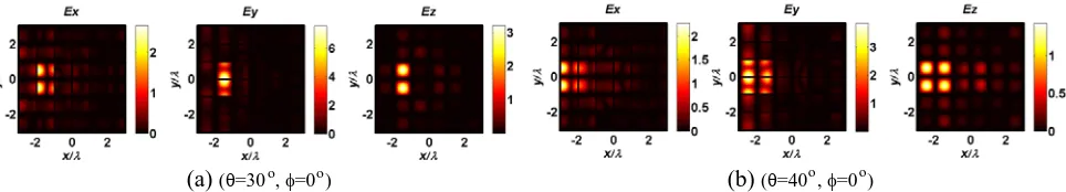
Figure 2 shows the Ex-,Ey-, and Ez-field distributions on the cross-section plane for two selected incident angles. Ey is always dominant over Ex and Ez, because the incident wave is y-polarized. Moreover, these field distributions vary slightly with gradual changes in the angles of incidence. The maximum of the electric field distribution shifts along the negative x-direction asθ varies from 30◦ to 45◦. Figure 3 shows a comparison of the weights for the entire 36 waveguides calculated by using the two methods discussed, herein. We see from this figure that the agreement is quite good.
Figure 4 shows a comparison between the simulated and reproducedE-fields, derived by using the waveguide mode extraction technique when θ = 30◦, ϕ = 0◦. It is evident that the waveguide mode extraction technique is able to accurately calculate the weights of the propagating modes and reproduce the field distribution, with less than 10% difference between the two. The 10% error can be attributed to the evanescent modes propagating in the waveguide, since the guide is not long enough for these modes to decay completely by the time they reach the cross-section plane.
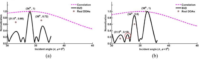
A case of three targets with angular separations as small as 2◦ was used to validate the approach. The three incident angles are set to be 31.5◦, 34◦ and 36◦ in θ, with ϕ= 0◦. Their scattering cross-sections are set to be (0.66, 1.0, and 0.72) in Figure 5(a) and (0.15, 0.6, and 1.0) in Figure 5(b). From Figure 5(a) it is obvious that the proposed method is capable of recovering the DOAs with high accuracy even if the targets are located in angular proximity of each other, a case which cannot be detected by using the CM alone. Figure 5(b) shows that when the scattering cross-section of the first target located at 31.5◦ is relatively low (15% of the maximum one), a false alarm emerges around 32◦, indicating that
(a) (θ=30 , o φ=0 )o (b) (θ=40 , o φ=0 )o
Figure 2. E-field distribution on cross-section plane of waveguide array for different incident angles: (a)θ = 30◦ and (b)θ = 40◦, with ϕ= 0◦.
(a) (b) (c)
Figure 3. Comparison of weights calculated in two different ways.
(a) (b) (c)
(a) (b)
Figure 5. Recovered DOAs by using proposed joint method.
scatterer would be difficult to locate if its radar cross-section is low, which is not entirely unexpected. Figure 5 also shows that the recovered DOAs are very close to the real ones; however, the recovered scattering cross-sections do not match the real ones, although their magnitudes do maintain the same relative order w.r.t. each other.
Finally, for the sake of completeness, we add Gaussian noise to the measured field values, with an amplitude level 30 dB below that of the signal.
5. CONCLUSIONS
In this work, we have presented a two-step approach, which is capable of achieving improved resolution in DOA estimation than that predicted by the half-power beamwidth of the aperture of a flat-base spherical Luneberg Lens with a planar waveguide array feed. The two-step approach, which involves waveguide mode extraction and signal processing techniques, has been shown to accurately detect multiple targets with an angular separation as small as 2◦, as long as the SNR is better than 30 dB. This concept can be naturally and readily extended to 2D/DOA scenarios, of course with increased computational burden.
REFERENCES
1. Balanis, C. A., Modern Antenna Handbook, Wiley, 2008.
2. Luneburg, R. K., Mathematical Theory of Optics, University of California Press, 1964.
3. Ma, H. F., B. G. Cai, T. X. Zhang, et al., “Three-dimensional gradient-index materials and their applications in microwave lens antennas,” IEEE Trans. Antennas Propag., Vol. 61, 2561–2569, 2013.
4. Dockrey, J. A., M. J. Lockyear, S. J. Berry, et al., “Thin metamaterial Luneburg lens for surface waves,” Physical Review B, Vol. 87, 125137, 2013.
5. Wu, L., X. Tian, M. Yin, et al., “Three-dimensional liquid flattened Luneburg lens with ultra-wide viewing angle and frequency band,”Appl. Phys. Lett., Vol. 103, 084102, 2013.
6. Dhouibi, A., S. N. Burokur, A. Lustrac, et al., “Compact metamaterial-based substrate-integrated Luneburg lens antenna,” IEEE Antennas and Wireless Propag. Lett., Vol. 11, 1504–1507, 2012. 7. Hua, C., X. Wu, N. Yang, and W. Wu, “Air-filled parallel-plate cylindrical modified Luneberg lens
antenna for multiple-beam scanning at millimeter-wave frequencies,”IEEE Trans. Microw. Theory Tech., Vol. 61, No. 1, 436–443, 2013.
8. James, G., A. Parfitt, J. Kot, and P. Hall, “A case for the Luneburg lens as the antenna element for the square-kilometre array radio telescope,”Radio Science Bulletin, Vol. 293, 32–37, Jun. 2000. 9. Liang, M., X. Yu, S.-G. Rafael, W.-R. Ng, M. E. Gehm, and H. Xin, “Direction of arrival estimation using Luneburg lens,”IEEE International Microwave Symposium (IMS) Digest (MTT), 1–3, Jun. 17–22, 2012.
11. Jain, S., R. Mittra, and M. Abdel-Mageed, “Broadband flat-base Luneburg lens for wide angle scan,”2014 IEEE Antennas and Propagation Society International Symposium (APS/URSI 2014), Memphis, TN, Jul. 6–11, 2014.
12. Luneburg, R. K., Mathematical Theory of Optics, University of California Press, 1964.
13. Guru, B. and H. Hiziroglu, Electromagnetic Field Theory Fundamentals, 2nd Edition, Cambridge University Press, 2004.