Title: HARD DECISION AND SOFT DECISION DECODING ALGORITHMS FOR LDPC AND QC-LDPC CODES

(1)

182

Available Online atwww.ijcsmc.com

International Journal of Computer Science and Mobile Computing

A Monthly Journal of Computer Science and Information Technology

ISSN 2320–088X

IJCSMC, Vol. 4, Issue. 9, September 2015, pg.182 – 191

RESEARCH ARTICLE

HARD DECISION AND SOFT DECISION

DECODING ALGORITHMS FOR LDPC

AND QC-LDPC CODES

**Er. Sonia*, Er. Swati Gupta**

*M.Tech Student, Deptt. of ECE, Geeta Institute of Management and Technology,Kurukshetra University, Haryana, India

[email protected]

Assistant Professor, Deptt. of ECE, Geeta Institute of Management and Technology,Kurukshetra University, Haryana, India

[email protected]

Abstract:- In this paper Hard Decision and Soft Decision decoding techniques for Quasi-Cyclic-Low Density Parity Check (QC-LDPC) code and

Low Density Parity Check (LDPC) code is introduced. QC-LDPC code is proposed to reduce the complexity of the Low Density Parity Check code

while obtaining the similar performance. The decoding processes of these codes are easy to simplify and implement. The algorithms used for

decoding techniques implemented on MATLAB for simulation results. LDPC & QC-LDPC codes can use the same decoding algorithms using the

parity check matrix. The decoding techniques is conducted by different algorithms such as Bit Flipping (BF) is example of the Hard decision

decoding techniques and Belief Propagation (BP) Log, Belief Propagation (BP) Probabilistic (PROB), Belief Propagation (BP) Log Simple is

example of the Soft decision decoding techniques.

Keywords:-“Low Density Parity Check Code”, “Quasi-Cyclic Low Density Parity Check code”, “Bit Error Rate”, “SNR”, “Decoding techniques”.

I. INTRODUCTION

Gallager first proposed LDPC codes in his PHD thesis 1962 [1], [2]. LDPC codes were carry out to achieved near the Shannon’s limit but at that time almost for thirty years the work done by Gallager was ignored until D.Mackay reintroduced these codes in 1996 [3]. Low density parity check codes are linear block codes using Generator Matrix G in an encoder and Parity Check Matrix H in a decoder. Tanner Graph is the bipartite graph introduced to graphically represent these codes[12]. They also help to describe decoding algorithm.

(2)

183

in a matrix which gives compact representation of H matrix [5], [6]. When designing a QC-LDPC code the parity check matrix H should have some properties that optimize the behavior of the belief propagation based decoder. QC-LDPC codes, based on circulant permutation matrices. If the weight w of circulant is equal to 1, then the circulant is called permutation matrix. The generator of the circulant is characterized by the first row on the first column of the same circulant.

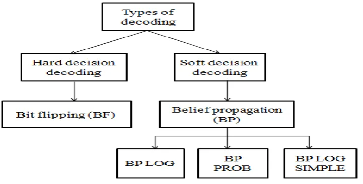
II. DECODING TECHNIQUES

The decoding techniques used in this paper are Sum Product Algorithm (SPA) and Bit Flipping (BF) algorithm [14]. Sum product algorithm also called belief propagation. Bit flipping algorithm is also called iterative decoding. LDPC & QC-LDPC codes can use the same decoding algorithm using the parity check matrix.

Iterative Decoding:-There are different iterative decoding algorithms having two derivations. Iterative Decoding algorithms based on their alphabet are generally classified as in hard decision and soft-decision decoding algorithms. There are various algorithms to deal with decoding of LDPC and QC-LDPC codes [15]. They are classified according to their complexities to get decoded for different codes. Detail explanation of hard and soft decision decoding algorithms with example.

Fig 1: Types of decoding techniques Hard Decision Decoding

In this hard decoding scheme [3] the check nodes finds the bit in error by checking the parity which may be even or odd and the messages from variable nodes are transmitted to check nodes, check node checks the parity of the data stream received from variable nodes connected to it. And then if number of 1’s received at check nodes satisfies the required parity, then it sends the same data back

to message nodes, else it adjusts each bit in the received data stream to satisfy the required parity and then transmits the new message back to message nodes. The bit flipping algorithm is an example of hard decision decoding [11], [13]. The Bit flipping decoder is going to be immediately terminated, whenever a valid code word has been found. By checking if all the parity check equations are satisfied then process get terminated.

BIT FLIPPING:-

(3)

184

Below example shows this process step by step [4]. The three steps are explained in detail:-

H = [

]

Step1:- Initialization

A value is assigned to each bit. After this all information is sent to the connected check nodes.

 Check nodes 3, 4 and 6 are connected to the bit node 1.

Check nodes receives bit values send by bit nodes. Step2:- Parity Update

The parity is calculated from this parity check equation and if the parity check equation has even number of 1`s, the parity will be satisfied. Check nodes 1 and 3 satisfies the parity check equation but check nodes 2 and 4 does not satisfy the parity check equation. For example:- Bit 1 will change its value from 1 to 0 if more number of received messages indicate “not satisfied” and the update information will be send to the check node.

Step3:- Bit Update

Step2 will be repeated again and again this time until all the parity check equations are satisfied. When all the parity check equations are satisfied, the algorithm will terminate and the final value of the decoded will be 001011.

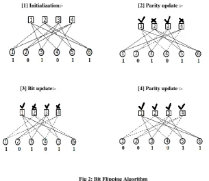
Below figure 2 shows step by step Bit Flipping in details:-

[1] Initialization:- [2] Parity update :-

[3] Bit update:- [4] Parity update :-

Fig 2: Bit Flipping Algorithm Soft Decision Decoding

(4)

185

bit is a 0 or a 1. The sum product algorithm is a soft decision decoding message passing algorithm. Priori probabilities for the received bits is the input probabilities as here they were known in advance before running the LDPC and QC-LDPC decoder. The bit probabilities returned by the decoder are called the posterior probabilities.

Sum Product Message Passing Algorithm (SPA):-

The sum-product algorithm is similar to the bit-flipping algorithm [8], but the major difference is that the messages representing each decision with probabilities in SPA whereas bit-flipping decoding on the received bits given as input, accepts an initial hard decision and the sum -product algorithm is a soft decision algorithm which accepts the probability of each received bit as input.

For a binary variable X it is easy to find P(x = 1) = 1−P(x = 0) and so we only need to store one probability value for x. Log

likelihood ratios are used to represent the metrics for a binary variable by a single value [9].

L(x) = p(X=0)

)

There are step by step explained in detail sum product algorithm:-

Step1:- Initialization

Communication to every check node j from every bit node I called LLR of the received signal i.e. “ ”. The properties of the

communication channel are hidden in this signal. The channel is AWGN with signal to noise ratio ⁄ .

Step2:- Check to Bit

The communication of the check node with the bit node is the probability for satisfaction of the parity check equation if we assume that bit =1 expressed in the following equation as LLR.

∏

Where is the current estimate, available to check j, of the probability that bit is a one. If bit is a zero, The probability that the

parity-check equation is satisfied is thus ( ) here it is expressed as a log likelihood ratio,

= LLR ( ) = Log (

)………… (2)

And substituting (2) we get

= log ( ∏

∏

………. (3)

where

Mj ,i = LLR ( ) = log (

)

Step3:- Codeword Test

Here each bit hasaccess to the input a priori Log Likelihood Ratio, ri, and the LLRs from every connected check nodes. The total Log Likelihood Ratio of the i-th bits is the sum of these LLRs.

L = LLR ( ) = ∑ ……….. (4)

Step4:- Bit to Check

The communication of each bit node I to the connected check node is the calculated Log Likelihood Ratio:- L = LLR ( ) = ∑ ……….. (5)

(5)

186

will decrease the complexity of the decoding process since a sum is more convenient to implement in hardware. The two decoding algorithms have almost equal bit error rate performances.

Probabilistic domain Belief Propagation (BP) decoding algorithm:- A posteriori probability and for each bit for an Additive

White Gaussian Noise channel.

( | )

…………. (a)

Logarithmic BP decoding algorithm is an enhanced version of the probabilistic BP algorithm, introducing logarithmic likelihood ratios (LLR) which reduce most multiplications to additions.

Logarithmic Domain Belief Propagation decoding algorithm:- In case of probability (PROB) domain sum product algorithm decoder, mostly multiplication is involved, but in case of log domain decoder multiplication is replaced with addition as log-function is used instead of normal function, hence complexity of implementation reduces.

It should be clear log-domain sum product algorithm has lower complexity and is more numerically stable than the probability-domain sum product algorithm.

III. SIMULATION RESULTS

Simulations have been carried out using MATLAB and the parameters used in the simulation are shown in Table 1. Code generated by various methods was simulated. We simulate the code error-correcting performance, with the assumption that each code is modulated by BPSK and transmitted over AWGN channel. The simulation parameters used here are shown in table:

Table 1: Simulation parameter

Simulation Tool used MATLAB

Iterations 10

Modulation BPSK

Channel Model AWGN

Number of rows 30

Number of columns 60

Decoding Algorithms

BF, BP LOG DOMAIN, BP PROB DOMAIN, BP LOG SIMPLE

Simulation result for LDPC code using different decoding algorithms:-

Now simulation results shows below for LDPC code using Bit flipping, Belief propagation logarithmic, Belief propagation probabilistic, belief propagation log simple.

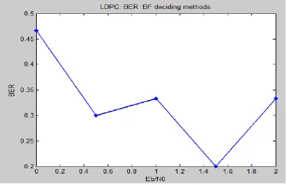
Figure 3 shows Bit error rate versus ⁄ for LDPC using BF decoding algorithm. For various SNR, bit error rate is calculated. In this figure for 0 ⁄ bit error rate is 0.4667, for 0.5 ⁄ bit error rate is 0.3000, for 1 ⁄ bit error rate is 0.3333, for 1.5

(6)

187

Fig 3: LDPC, Bit flipping decoding methods

Figure 4 shows Bit error rate versus ⁄ for LDPC code using BP-LOG-SIMPLE decoding algorithm. For various SNR, bit error rate is calculated. In this figure for 0 ⁄ bit error rate is 0.2000, for 0.5 ⁄ bit error rate is 0.2333, for 1 ⁄ bit

error rate is 0.1333, for 1.5 ⁄ bit error rate is 0.1000 and for 2 ⁄ bit error rate is 0.0667.

Fig 4: LDPC, BP LOG SIMPLE decoding methods

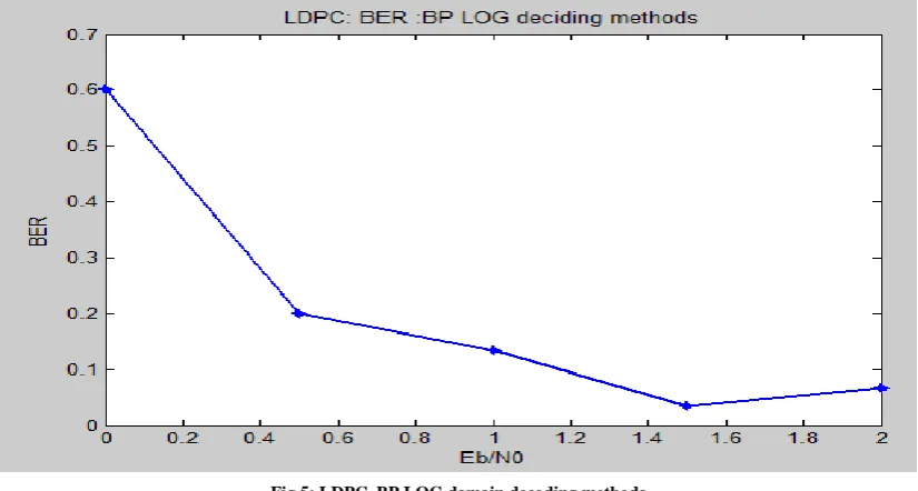
Figure 5 shows Bit error rate versus ⁄ for LDPC code using Belief Propagation LOG domain decoding algorithm. For various

(7)

188

Fig 5: LDPC, BP LOG domain decoding methods

Figure 6 shows Bit error rate versus ⁄ for LDPC code using Belief Propagation PROB domain decoding algorithm. For various

SNR, bit error rate is calculated. In this figure for 0 ⁄ bit error rate is 0.6000, for 0.5 ⁄ bit error rate is 0.2000, for 1 ⁄ bit error rate is 0.1333, for 1.5 ⁄ bit error rate is 0.0333 and for 2 ⁄ bit error rate is 0.0667.

Fig 6: LDPC, BP PROB domain decoding methods

Belief propagation logarithmic algorithm and belief propagation probabilistic algorithm shows same bit error rate for same ⁄ . Belief propagation logarithmic decoding algorithm simplify in the belief propagation logarithmic simple decoding algorithm.

Simulation result for QC-LDPC code using different decoding

(8)

189

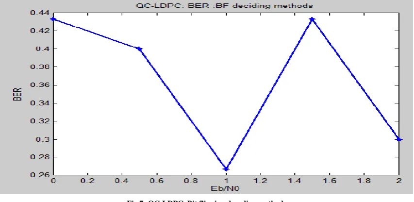
Figure 7 shows Bit error rate versus ⁄ for QC-LDPC code using bit flipping decoding algorithm. For various SNR, bit error rate is calculated. In this figure for 0 ⁄ bit error rate is 0.4333, for 0.5 ⁄ bit error rate is 0.4000, for 1 ⁄ bit error rate is 0.2667, for 1.5 ⁄ bit error rate is 0.4333 and for 2 ⁄ bit error rate is 0.3000.

Fig 7: QC-LDPC, Bit flipping decoding methods

Figure 8 shows Bit error rate versus ⁄ for QC-LDPC code using Belief Propagation LOG SIMPLE decoding algorithm. For various SNR, bit error rate is calculated. In this figure for 0 ⁄ bit error rate is 0.1667, for 0.5 ⁄ bit error rate is 0.1333, for 1

⁄ bit error rate is 0.1667, for 1.5 ⁄ bit error rate is 0.0667 and for 2 ⁄ bit error rate is 0.0667.

Fig 8: QC-LDPC, BP LOG SIMPLE decoding methods

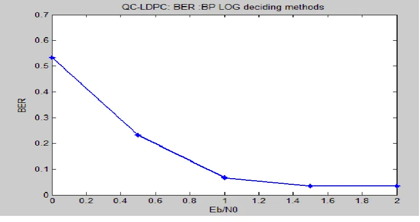
Figure 9 shows Bit error rate versus ⁄ for QC-LDPC code using Belief Propagation LOG domain decoding algorithm. For various SNR, bit error rate is calculated. In this figure for 0 ⁄ bit error rate is 0.5333, for 0.5 ⁄ bit error rate is 0.2333, for 1

(9)

190

Fig 9: QC-LDPC, BP LOG decoding methods

Figure 10 shows Bit error rate versus ⁄ for QC-LDPC code using Belief Propagation LOG PROB domain decoding algorithm. For various SNR, bit error rate is calculated. In this figure for 0 ⁄ bit error rate is 0.5333, for 0.5 ⁄ bit error rate is 0.2333,

for 1 ⁄ bit error rate is 0.0667, for 1.5 ⁄ bit error rate is 0.0333 and for 2 ⁄ bit error rate is 0.0333.

Fig 10: QC-LDPC, BP PROB decoding methods

Belief propagation logarithmic algorithm and belief propagation probabilistic algorithm shows same bit error rate for same ⁄ . Belief propagation logarithmic decoding algorithm simplify in the belief propagation logarithmic simple decoding algorithm.

IV. CONCLUSION

(10)

191

REFERENCES

[1] Gallager, R.G., “Low-Density Parity-Check codes,” IRE Trans. Info. Theory, Vol. IT-8, January 1962.

[2] Gallager, R. G., Low-Density Parity-Check Codes, Cambridge, MA: The MIT Press, 1963.

[3] Kai Zhang, Xinming Member and Zhongfeng wang, “High Throughput Layered Decoder Implementation for Quasi-Cyclic LDPC Codes”, IEEE, vol. 27, no. 6, August 2009.

[4] Mohammad Rakibul ISLAM, Jinsang KIM “Quasi Cyclic- LDPC code for High SNR Data Transfer”, RADIOENGINEERING, vol.19, no. 2, June 2010.

[5] Mohammad Rakibul ISLAM, “Quasi Cyclic- LDPC code for High SNR Data Transfer,” Vol.19, No. 2, June 2010. [6] NAVEED NIZAM, “On the Design of Cyclic-Quasi Cyclic LDPC Codes,” 3 June 2013.

[7] Yaqi Li, Bo Rong, Bo Liu, Yiyan Wv and Gilles Gagnon, “Rate-compatible LDPC-RS Product Codes Based on Raptor-like LDPC codes”,IEEE 2013.

[8] JohnC. Porcello and Senior member IEEE, “Designing and Implementing Low Density Parity Check (LDPC) Decoders using FPGAs”, IEEE 2014.

[9] Namrata P. Bhavsar and Brijesn Vala “Design of Hard and Soft Decision Decoding Algorithms of LDPC”, International Journal of Computer Applications, vol.90, no.16, March 2014.

[10]Namrata P. Bhavsar, “Design of Hard and Soft Decision Decoding Algorithms of LDPC,” International Journal of Computer Applications, vol.90, no.16 March2014.

[11]Chinna Babu.J, S.Prathyusha, “Hard Decision and Soft Decoding Algorithms of LDPC and Comparison of LDPC With Turbo Codes, RS Codes and BCH Codes,” IRF International Conference, 27th july-2014.

[12]Mini Manpret and Prabhdeep Singh, “Decoding techniques of error control codes called LDPC,” ijesrt, vol. 3, issue 8, August 2014.

[13]Monica V.Mankar, Abha Patil and G.M.Asutkar, “Single mode Quasi-cyclic LDPC Decoder Using Modified Belief Propagation,” IEEE 2014.

[14]Sonia, Geeta Arora, “A survey of different decoding schemes for LDPC block codes,” IJECS Volume 4 issue 5 May 2015.

[15]Sonia, Geeta Arora, “Implementation of different decoding techniques for QC-LDPC codes,” IJESRT Volume 4 issue 6 June 2015.

Title: HARD DECISION AND SOFT DECISION DECODING ALGORITHMS FOR LDPC AND QC-LDPC CODES﻿

182