On the Role of Expander Graphs in Key
Predistribution Schemes for Wireless Sensor
Networks
Michelle Kendall and Keith Martin
Information Security Group, Royal Holloway, University of London, Egham, Surrey, TW20 0EX, UK
Abstract. Providing security for a wireless sensor network composed of small sensor nodes with limited battery power and memory can be a non-trivial task. A variety of key predistribution schemes have been proposed which allocate symmetric keys to the sensor nodes before deployment. In this paper we examine the role of expander graphs in key predistri-bution schemes for wireless sensor networks. Roughly speaking, a graph has good expansion if every ‘small’ subset of vertices has a ‘large’ neigh-bourhood, and intuitively, expansion is a desirable property for graphs of networks. It has been claimed that good expansion in the product graph is necessary for ‘optimal’ networks. We demonstrate flaws in this claim, argue instead that good expansion is desirable in the intersection graph, and discuss how this can be achieved. We then consider key predistribu-tion schemes based on expander graph construcpredistribu-tions and compare them to other schemes in the literature. Finally, we propose the use of expan-sion and other graph-theoretical techniques as metrics for assessing key predistribution schemes and their resulting wireless sensor networks.
Keywords: Wireless Sensor Networks, Key Predistribution, Expander Graphs
1
Introduction
A wireless sensor network (WSN) is a collection of small, battery powered de-vices called sensor nodes. The nodes communicate with each other wirelessly and the resulting network is usually used for monitoring an environment by gather-ing local data such as temperature, light or motion. As the nodes are lightweight and battery powered, it is important to consider battery conservation in order to allow the network to remain effective for the appropriate period of time, and to ensure that the storage required of the nodes is not beyond their memory capacity.
proposed for such scenarios. In some cases there is an online key server or base station to distribute keys to the nodes where needed; if not,key predistribution schemes (KPSs) are required, which assign keys to nodes before deployment. Due to the resource-constrained nature of the nodes, it may be infeasible to use asymmetric cryptographic techinques in some WSN scenarios, and so we consider symmetric key predistribution schemes.
Since networks may be modelled as graphs, tools from graph theory have been used both to analyse and to design networks. In particular, we explore the role of expander graphs in KPSs for WSNs. The expansion of a graph is a measure of how well connected it is, and how difficult it is to separate subsets of vertices; we will see the precise definition in Sect. 2.3. The term ‘expander graphs’ is used informally to refer to graphs with good expansion.
In 2006, expander graph theory was introduced to the study of KPSs for WSNs from two perspectives. On the one hand, Camtepe et al [5] showed that a mathematical construction for an expander graph could be used to design a KPS, resulting in a network which is well connected under certain constraints. On the other hand, Ghosh [13] claimed that good expansion is a necessary condition for ‘optimal’ WSNs. We examine these claims and determine the role of expander graphs in KPSs for WSNs.
Firstly, we show that Ghosh’s claim is flawed but identify where expansion properties are desirable for WSNs, namely in the intersection graph rather than the product graph. We then analyse the effectiveness of constructions for KPSs based on expander graphs, showing that they provide perfect resilience against an adversary but lower connectivity and expansion than many existing KPSs, for the same network size and key storage. We argue that expansion is an important metric for assessing KPSs to be used alongside the other common metrics of key storage, connectivity and resilience for a given network size. However, we note the difficulty of finding the expansion coefficient of a graph and so propose es-timating the expansion and using other graph-theoretical techniques to indicate weaknesses.
We begin by introducing the relevant terminology and concepts in Sect. 2. In Sect. 3 we outline Ghosh’s claims and show by means of a counter-example that his conclusion is misdirected towards expansion in product graphs rather than intersection graphs. In Sect. 4 we discuss how to maximise the probability of a high expansion coefficent in the intersection graph, and in Sect. 5 we analyse the extent to which KPSs based on expander graph constructions achieve this, in comparison to other schemes from the literature. Finally, in Sect. 6 we suggest practical metrics for analysing and improving KPSs and the resulting WSNs, and conclude in Sect. 7.
2
Background
2.1 Key Predistribution Schemes for Wireless Sensor Networks
the nodes have been deployed in the environment, they broadcast identifiers which uniquely correspond to the keys they store, and determine the other nodes (within communication range) with which they share at least one common key, in order to form a WSN.
There are many ways of designing a KPS, and different KPSs suit different WSN applications. We consider KPSs which assign symmetric keys, since small sensor nodes are resource-constrained with low storage, communication and com-putational abilities, and are often unable to support asymmetric cryptography. In order to make best use of the nodes’ limited resources, it is usually desirable to minimise thekey storagerequirement whilst maximising theconnectivity and resilience of the network. We now define these concepts more precisely.
– Key storage is the maximum number of keys which an individual node is required to store for a particular KPS.
– Connectivity of a network can be measured or estimated bothglobally and locally. We will refer again to global connectivity in Sect. 6 but in general we will use the measure of local connectivityPr1. This is defined to be the probability that two randomly-chosen nodes are ‘connected’ because they have at leastqkeys in common. Most KPSs require nodes to share just one key before they can establish a secure connection, ie.q = 1, and so Pr1 is simply the probability that a random pair of nodes have at least one key in common. Some schemes such as theq-composite scheme of Chan et al. [6] introduce a threshold such that nodes may only communicate if they have at leastq >1 common keys. Where two nodes share more thanqkeys, some protocols dictate that they should use a combination of those keys, such as a hash, to encrypt their communications.
– Resilienceis a measure of the network’s ability to withstand damage from an adversary. We use the adversary model of a continuous, listening adversary, which can listen to any communication across the network and continually over time ‘compromise’ nodes, learning the keys which they store. We mea-sure the resilience with the parameter fails: we suppose that an adversary
has compromisedsnodes, and then compute the probability that a link be-tween two uncompromised nodes in the network is compromised, that is, the adversary knows the key(s) being used to secure it. Equivalently, fails
measures the fraction of compromised links between uncompromised nodes throughout the network, after an adversary has compromiseds nodes. No-tice that high resilience corresponds to a low value of fails. We say that a
network has perfect resilience against such an adversary if fails = 0 for all
1≤s < n−2.
To illustrate the trade-offs required between these three parameters, we con-sider some trivial examples of KPSs.
1. Every node is assigned a single keykbefore deployment.
of a single node would reveal the keyk, rendering all other links insecure. Formally, fails = 1 for all 1 ≤s ≤ n−2, where n is the total number of
nodes.
2. A unique key is assigned to every pair of nodes.
That is, for all 1≤i, j≤n, nodesni andnj are both preloaded with a key
kij, wherekij 6=klm for alll6=i, m6=j. This is called thecomplete pairwise
KPS. Such a KPS would have perfect resilience and maximum connectivity, as Pr1 = 1 for all pairs of nodes. However, each node would have to store
n−1 keys, which is infeasible whennis large. 3. Every node is assigned a single unique key.
Whilst providing minimal key storage and perfect resilience, this KPS has no connectivity, asPr1= 0 for all pairs of nodes.
We see, then, that it is trivial to optimise any two of these three parameters. However, for many WSN applications these schemes are inappropriate, and so we consider KPSs which find trade-offs between all three of these metrics. A variety of such KPSs have been proposed, both deterministic and random, a survey of which is given in [4][7][19][23].
We now describe the Eschenauer Gligor KPS [12] as an example of a KPS which provides values for the three metrics which are appropriate for many WSN scenarios. It will also be used as a comparison for KPSs based on expander graph constructions in Sect. 5.
Example 1. The Eschenauer Gligor KPS [12] works in the following way. A key poolK is generated. To each nodeni is assigned a random subset ofkkeys from
K. The probability of two nodes sharing at least one key is
Pr1= 1−
|K|−k k
|K| k
. (1)
An equivalent formula is given in [12]. We verify (1) by considering the prob-ability of two arbitrary nodes ni and nj sharing no common keys. If node ni
stores a set Si of k keys, node nj stores Sj andSi∩Sj =∅, then every key of
Sj must have been picked from the key poolK \Si, that is from a set of|K| −k
keys. Therefore the probability of two nodes having no keys in common is equal to the number of ways of choosingk keys from a key pool of |K| −k, divided by the number of ways of choosingk keys from the full key pool.
As explained in [6], the resilience after the compromise ofsnodes is
fails=
1−
1− k
|K|
sq
. (2)
fail1=|K|k . Ifq >1keys are shared between the nodes then the value offail1 will be smaller, asfail1=
k |K|
q .
Table 1 demonstrates the value of Pr1 and upper bound for fail1 for some different sizes of key pool and key storage. (We assume for this example that all nodes are within communication range of one another.) It can be seen that by adjusting the values of |K|andk, with ksmall, we can achieve arbitrarily large Pr1 whilst keepingfail1 relatively small. This makes the Eschenauer Gligor KPS appropriate for many WSN scenarios.
Table 1.Example values for an Eschenauer Gligor KPS
|K| k Pr1 fail1
500 25 0.731529 0.050 500 50 0.996154 0.100 1000 25 0.473112 0.025 1000 50 0.928023 0.050
In accordance with most papers in the literature, we will use key storage, connectivity and resilience along with network size as metrics for comparing KPSs. Network size is relevant since for small networks the complete pairwise KPS is practical, and because some KPSs are not adaptable for all sizes of network. For example we will see in Sect. 5 that the KPS proposed by Camtepe et al [5] is only possible for networks of sizen=t+1 wheretis a prime congruent to 1 mod 4.
Later, in Sect. 6, we will propose that in addition to network size, key storage, connectivity and resilience, it is important to consider expansion as a metric when comparing KPSs.
2.2 Graph Theory
We now introduce some graph-theoretic definitions, beginning with general ter-minology in this section before giving the specific definitions related to expander graphs in Sect. 2.3.
Agraph G= (V, E) is a set of vertices V ={v1, . . . , vn} and a set of edges
E. We use the notation (vi, vj)∈Eto express that there is an edge between the
verticesvi andvj, and we say that the edge (vi, vj) isincident to its endpoints
vi andvj. Wherever an edge (vi, vj) exists,viandvj can be said to beadjacent.
are not directed from one vertex to the other, there are no edges from the a node to itself, and any edge between two vertices is unique.
Given subsets of verticesX, Y ⊂V, the set of edges which connectX andY
is denoted
E(X, Y) ={(x, y) :x∈X, y∈Y and (x, y)∈E} ,
and thecomplementXofXis the vertices which are not inX, that is,X =V\X. An ordered set of consecutive edges{(vi1, vi2),(vi2, vi3), . . . ,(vi(p−1), vip)}in
which all the verticesvi1, vi2, . . . , vipare distinct is called apathof lengthp−1. A
cycleis a ‘closed’ path which begins and ends at the same vertex, ie. a cycle is a path{(vi1, vi2),(vi2, vi3), . . . ,(vi(p−1), vip)}wherevi1, vi2, . . . , vi(p−1)are distinct butvi1=vip. We say that a graph isconnected if there is a path between every
pair of vertices, and complete if there is an edge between every pair of vertices. Thedegree d(v) of a vertex v is the number of edges incident to that vertex. If all nodes have the same degreer, we call the graphr-regular.
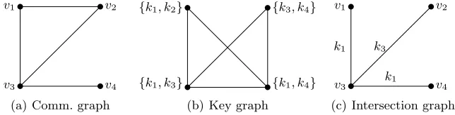
We draw a graph of a WSN by representing the nodes as vertices and the ‘connections’ as edges. To be precise in our analysis, we distinguish between the two possible types of ‘connection’ and consider the separate constituent graphs of a network: the communication graph G1 = (V, E1) where (vi, vj) ∈ E1 if
vi and vj are within communication range, and the key graph G2 = (V, E2) where (vi, vj)∈E2 ifvi andvj share at leastq common keys. An example of a
communication graph and a key graph are given in Fig. 1.
v1 v2
v3 v4
(a) Comm. graph
{k1, k2} {k3, k4}
{k1, k3} {k1, k4}
(b) Key graph
v1 v2
v3 v4
k1 k3
k1
(c) Intersection graph
Fig. 1.Example of corresponding communication, key and intersection graphs
If the communication graph is complete, it is often omitted from the analysis as there is no need to check whether nodes can communicate. However, as we will explain in Sect. 4, the communication graph is commonly modelled using a random graph, and it then becomes important to analyse how the communication and key graphs relate to each other.
We say that two nodes vi and vj can communicate securely if (vi, vj) ∈
If two nodes are not adjacent in the intersection graph then there are usually ways for them to communicate by routing messages through intermediary nodes and/or establishing a new key. Since any protocol for either of these methods requires extra communication overheads, it is desirable to minimise thediameter of the intersection graph, that is to minimise the longest path length between nodes. Similarly, it may also be desirable to minimise the average path length of the intersection graph.
Finally, we introduce another way of combining two graphs, which will be needed for Sect. 3 where we consider Ghosh’s claims.
Definition 1. The (Cartesian) product graphof two graphsG= (VG, EG)and
H = (VH, EH) is defined as G.H = (VG ×VH, EG.H), where the set of edges
EG.H is defined in the following way:(uv, u0v0)∈EG.H if
(u=u0 or(u, u0)∈EG)
and
(v=v0 or (v, v0)∈EH) .
We will now define expander graphs and explain why their properties are desirable for WSNs.
2.3 Expander Graphs
For a thorough survey of expander graphs and their applications, see [14]. The expansion of a graph is a measure of the quality of its connectivity.
Definition 2. A finite graph G = (V, E) is an -expander graph, where the edge-expansion coefficient is defined by
= min
S⊂V:|S|≤|V2|
|E(S, S)|
|S|
,
where|E(S, S)|denotes the number of edges from the setS to its complement. The phrase ‘expander graph’ is used informally to refer to graphs with good expansion, that is, graphs with a high value of, as we explain below. We note that definitions vary across the literature, in particular some defintions use the strict inequality |S| < |V2|. Another name for the edge-expansion coefficient is theisoperimetric number, and in a graph where every vertex has the same weight this is equivalent to theCheeger constant; see [9] for further details.
We now explore what the definition of the edge-expansion coefficientmeans, and why a high value ofis desirable, through the following observations:
– If = 0 then we see from the definition that there exists a subset S ⊂ V
without any edges connecting it to the rest of the graph. This implies that the graph is not connected.
– Ifis ‘small’, for example= 1
100, then there exists a set of verticesSwhich is only connected to the rest of the graph by one edge per 100 nodes inS. This is undesirable for a WSN for the following reasons:
• The set S is vulnerable to being ‘cut off’ from the rest of the network by a small number of attacks or faults. IfS containsc×100 nodes then there are onlycedges betweenSandS. A small number of compromises or failures amongst the particular≤2cnodes incident to these edges will render all communication betweenS andS insecure.
• Since S is connected to the rest of the network by comparatively few edges, a higher communication burden is placed on the small set of≤2c
nodes, since a higher proportion of data needs to be routed through them. This will drain the batteries of the nodes nearest to the edges between S and S faster than those of an average node, so that after some period of time they will run out of energy, disconnecting S from the rest of the network even though many nodes in S may still have battery power remaining.
• Reliance on a small number of edges to connect large sets of nodes may create bottlenecks in the transmission of data through the network, mak-ing data collection and/or aggregation less efficient.
– Ifis larger, particularly if >1, then there is no ‘easy’ way to disconnect large sets of nodes, and communication burdens, battery usage and data flow are more evenly spread.
We see from these observations that intersection graphs with higher values ofare more desirable for WSNs. A graph with a ‘large’ value ofis often said to have ‘good expansion’. The the size ofis subject to the following bounds.
Proposition 1. For any connected graph G= (V, E)with |V| ≥2,
0< ≤min
v∈Vd(v) .
Proof. We begin by considering the lower bound. Suppose for a contradiction that = 0. Then there exists a set S⊂V such|E(S, S)|= 0. This contradicts the fact thatGis connected. Sincecannot be negative, we have that >0.
For the upper bound, consider the set S = {v} where v ∈ V. It is clear that |E(S, S)|=d(v), where d(v) is the degree of v as defined in Sect. 2.2, and so |E(|S|S,S)| = d(1v) =d(v).Since the definition of the edge-expansion coefficient
uses the minimum value over all S ⊂ V with |S| ≤ |V2|, we have that ≤
minv∈V d(v). ut
The papers by Camtepe et al. [5] and Shafiei et al. [21] propose KPSs based on expander graph constructions. These methods of designing a KPS ensure that the key graph has good expansion, and we further examine these proposals in Sect. 5. First, we consider the claims made by Ghosh in [13] about the necessity of good expansion for ‘optimal’ networks.
3
Expansion in Product Graphs
In [13] Ghosh considers KPSs with large network size, low key storage per node, high connectivity and high resilience. He considers jointly ‘optimising’ these parameters, although exactly what this means is unclear, since different appli-cations will prioritise them differently. Nevertheless, he argues that if a KPS is in some sense ‘optimal’, the product graph of the key graph and communication graph must have ‘good expansion properties’. We show by a counterexample that expansion in the product graph is not a helpful measure because the product graph is almost inevitably an expander graph. Additionally, we show that the product graph is unable to capture the required detail to analyse a WSN, and that it is the intersection graph where such analysis is relevant.
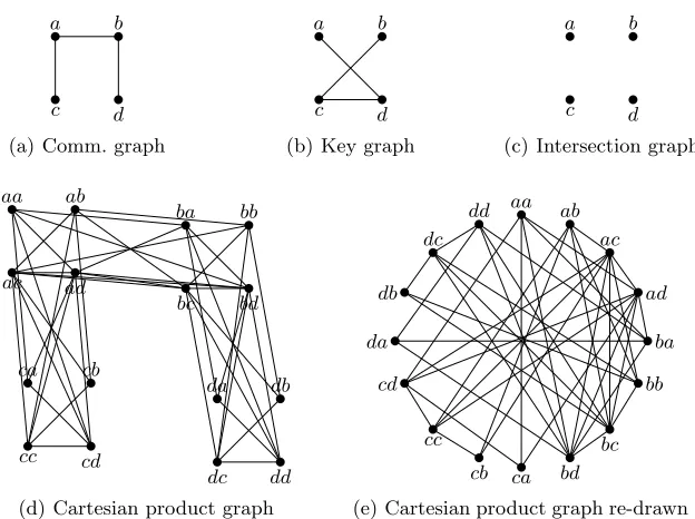
In Fig.s 2 and 3 we consider examples of product graphs and examine how they relate to their constituent communication and key graphs. Figure 2 shows a communication and a key graph, and their corresponding intersection and product graphs. The product graph is represented in Fig. 2(d) in a way which demonstrates its construction, and redrawn in Fig. 2(e) for clarity.
Figure 2(d) illustrates that the product graph construction results in four copies of the key graph, connected to each other in a pattern which resembles the communication graph. To provide an alternative perspective, we re-draw the same graph with the vertices arranged in a circle in Fig. 2(e). To understand the construction, recall Def. 1 which defines the vertices and edges of the product graph. We find that there is an edge in the product graph (ac, ab)∈EG.Hbecause
a=aand (c, b)∈EH. Similarly, (ca, ba)∈EG.Hbecause (c, b)∈EGanda=a.
However, we find that (aa, ab)∈/EG.H because whilsta=a, (a, b)∈/ EH.
In Fig. 2 the communication and key graphs are identical, giving the best possible case for intersection. We now calculate the expansion coefficient of the product graph. Consider setsS of 1,2, . . . ,8 vertices (recall from the definition that we should consider subsets S with |S| ≤ |V2|, and here |V| = 16). We observe that any single vertex is connected to the rest of the graph by at least three edges, any set of two vertices is connected to the rest of the graph by at least six edges, etc., so that
= min 3
1, 6 2,
9 3,
9 4,
11 5 ,
16 6 ,
12 7 ,
10 8
.
That is, = 108 = 54, so the product graph of Fig. 2 has expansion coefficient
= 54.
a b
c d
(a) Comm. graph
a b
c d
(b) Key graph
a b
c d
(c) Intersection graph
aa ab
ac ad
ba bb
bc bd
ca cb
cc cd
da db
dc dd
(d) Cartesian product graph
aa ab
ac
ad
ba
bb
bc bd ca cb cc cd da
db dc
dd
(e) Cartesian product graph re-drawn
Fig. 2.A product graph corresponding to an identical communication and key graph pair.
a way that the intersection graph, shown in Fig. 3(c), has no edges. Clearly for WSN purposes this would mean that no secure communication was possible.
However, the product graph does have edges, and indeed appears well con-nected. By observation, we find that it too has expansion coefficient = 5
4. Indeed, after some inspection, we find that the product graphs of Fig.s 2 and 3 are isomorphic, using a simple bijection to relabel vertices as follows:
Fig. 2(e) Fig. 3(e) (a∗) → (c∗) (b∗) → (d∗) (c∗) → (b∗) (d∗) → (a∗)
This means that all graph-theoretic properties of connectivity, expansion, degree, diameter etc. are identical between the two product graphs. From this we see that a product graph with good expansion can occur when the key and communication graphs intersect ‘fully’, ie. when EG∩EH =EG =EH, and when there are no
edges in the intersection, ie. EG ∩EH = ∅. This shows that the expansion of
a b
c d
(a) Comm. graph
a b
c d
(b) Key graph
a b
c d
(c) Intersection graph
aa ab
ac ad
ba bb
bc bd
ca cb
cc cd
da db
dc dd
(d) Cartesian product graph
aa ab
ac
ad
ba
bb
bc bd ca cb cc cd da
db dc
dd
(e) Cartesian product graph re-drawn
Fig. 3.A product graph corresponding to a communication and key graph pair with empty intersection.
the connectivity of WSNs without reference to the intersection graph. Ghosh’s claim that an ‘optimal’ combination of key and communication graph will result in a product graph with good expansion tells us very little, since good expansion in the product graph is almost inevitable, as we will now explain.
Proposition 2. A (Cartesian) product graph G.H = (VG×VH, EG.H) is
con-nected if and only if both G= (VG, EG)andH = (VH, EH) are connected.
Proof. If the product graph is connected then there is a path between all pairs of verticesu1v1, upvq ∈V ×V, say
(u1v1, u2, v2),(u2v2, u3v3), . . . ,(up−1vq−1, upvq) .
Using the definition of the product graph, this implies that either u1 =u2 or (u1, u2)∈EG, and indeed for all 1≤i≤p−1, either ui =ui+1 or (ui, ui+1)∈
EG. Thus eitheru1=upor there is a path fromu1toupinG. Since this is true
for all pairs of vertices u1, up ∈V, we have that G is connected. By the same
argument,H is also connected.
Suppose that G and H are both connected graphs. Then for each distinct pair of verticesu1, up ∈VG, there is a path between them, say
Similarly, for each distinct pair of verticesv1, vq ∈VH, there is a path, say
(v1, v2),(v2, v3), . . . ,(vq−1, vq) .
By the definition of EG.H, we have that (u1v1, u2v2) ∈ EG.H. Thus we can
construct a path
(u1v1, u2v2),(u2v2, u3v3), . . . ,(up−1vq−1, upvq)
in G.H between any pair of vertices, and thereforeG.H is connected. ut
Corollary 1. If GandH are connected, the product graph G.H has expansion coefficientG.H >0.
Proof. Recall from Prop. 1 that a connected graph is an expander graph for some value of. Therefore, ifGandH are connected, the product graph will be
an expander graph for some value of G.H>0. ut
We conjecture that with high probability, G.H > G, H and G.H >> 0.
We justify this by considering the comparatively large degrees of nodes in the product graph, and the product graph’s similarity to an expander graph con-struction.
For any node v ∈ V with degrees dG(v), dH(v) in the communication and
key graphs respectively, we can compute its degree in the product graph as
dG.H(v) =dG(v)dH(v) +dG(v) +dH(v) . (3)
Using Prop. 1, we have that
G.H≤min
v∈V(dG(v)dH(v) +dG(v) +dH(v)) ,
a much higher bound than for the constituent graphs. Since, on average, vertices of the product graph have higher degree than vertices in the constituent graphs, and since the construction of the product graph makes ‘isolated’ sets of ver-tices extremely unlikely, we see thatG.H is likely to be large, and in particular
greater than either ofG andH. By comparison, the expansion coefficient of the
intersection graph G∩H is forced to be no more than those of the constituent
graphs, G andH, as explained in the next section.
4
Expansion in Intersection Graphs
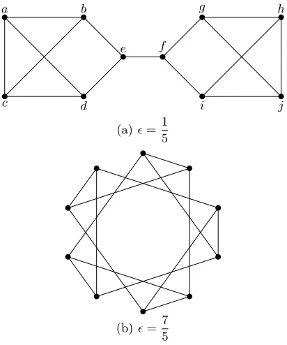
We claim that when comparing two networks of the same size with identical key storage, connectivity and resilience parameters, the intersection graph with the better expansion represents the better WSN. We justify this using the following example.
Example 2. Consider Fig. 4 and suppose that these are two intersection graphs, representing WSNs. Each graph is 3-regular on 10 nodes. We suppose that an Eschenauer Gligor KPS (as described in Sect. 2.1) has been used to construct the key graph, where each node stores three keys chosen randomly from a pool of 25 keys. To simplify the analysis, we say that where nodes have more than one key in common, they select just one of them for use in securing their communications.
a
c
b
d
e f
g
i
h
j
(a)=1 5
(b)= 7 5
Fig. 4.Examples of 3-regular graphs on 10 nodes with different expansion parameters.
Using the formulae given in Sect. 2.1 we calculate thatPr1= 1−( 22
3) (25
3)
≈0.33,
fail1 = 253 andfails= 1− 1−253 s
that = 7
5; any set of 5 vertices is connected by at least 7 edges to the rest of the graph.
For WSN applications, the network represented by Fig. 4(a) is less desirable, because
– it is more vulnerable to a listening adversary, who could decrypt a high pro-portion of communications through the network by the compromise of a single nodeeorf
– nodeseandf are more vulnerable to battery failure
– battery failure of just one of the two nodes e and f would disconnect the network
– communication bottlenecks are likely to occur around nodeseandf, making communication through the network less efficient.
Conversely, in Fig. 4(b) the communication burdens are distributed evenly across the nodes so that battery power will be used more evenly and there are no weak spots for an adversary to target in order to quickly damage the rest of the network. The graph can only be split into disjoint sets by the removal of 4 or more nodes, that is, almost half of the network. It is clear then that Fig. 4(b) represents the less vulnerable WSN.
From this example we see that some strengths and weaknesses of the ‘layout’ of the WSN are hidden if we only consider the size, key storage, connectivity and resilience, and in Sect. 6 we discuss the practicality of using expansion as another metric for assessing networks. Before that, we consider how best to probabilistically maximise the expansion in an intersection graph, and in Sect. 5 we will consider schemes which aim to produce key graphs with good expansion. We now consider how to achieve high expansion in an intersection graph
G∩H.
Proposition 3. An intersection graphG∩H = (V∩V, EG∩EH)has expansion
parameter
G∩H≤min{G, H} .
Proof. We begin by considering the degree of a node in the intersection graph, which is
dG∩H(v)≤min (dG(v), dH(v))
because each edge (v, w) incident to a vertex v in G will be removed in the intersection unless there is also an edge (v, w) inH. Using Prop. 1, we have that
G∩H≤minv∈V{dG∩H(v)}.
Without loss of generality, suppose thatG≤H. Consider a setSof vertices
inGwhich achieves the minimum |E(|S|S,S)|=G. If every edge ofE(S, S) remains
in the intersection then G∩H ≤ G, otherwise G∩H < G, since no edges are
added elsewhere in the intersection. Therefore we have thatG∩H ≤min{G, H}.
We see that it is necessary thatGandH have high expansion coefficients for
G∩H to be a good expander. If the communication graph is complete then the expansion of the key graph will be preserved in the intersection. If information about the locations of the nodes is known a priori or if there is some control over the communication graph, then keys can be assigned to nodes in a more efficient manner; see [18] for a survey of KPSs for such scenarios.
However, we usually assume that there is little or no control over the commu-nication graph and model it as a random graph, typically using either the Erd¨os R´enyi model [11] or the random geometric model, as in [5]. If the communication graph is random, all that can be done to aid good expansion in the intersection graph is to design the KPS so that the key graph has as high expansion as possi-ble for a particular network size and for given levels of key storage, connectivity and resilience.
5
Analysing the Expansion Properties of Existing KPSs
Many KPSs produce key graphs with high expansion coefficients for chosen levels of key storage and resilience, as demonstrated by the following examples.
– Random graphs are good expanders with high probability [14], and so Es-chenauer and Gligor’s random KPS [12] is likely to produce key graphs which are good expanders, as are other random KPSs such as those given in [6]. – Deterministic schemes based on combinatorial designs, as unified in [19],
typically guarantee properties such as constant node degree andµcommon intersection. That is, if two nodes are not adjacent then they haveµcommon neighbours, meaning that the graph has diameter 2, and is therefore a good expander. In particular, two deterministic KPSs based on constructions for ‘strongly regular’ graphs are given in [17].
– Camtepe et al. [5] and Shafiei et al. [21] propose KPSs based on expander graph constructions and demonstrate that these schemes compare well to other well-regarded KPS approaches.
We now consider the KPSs based on expander graph constructions in more detail, and compare them to the other schemes listed above. Camtepe et al. [5] use the Ramanujan construction which produces an ‘asymptotically optimal’ expander graph (see [14]) for network sizen=t+ 1 and key storagek=s+ 1, wheretandsare primes congruent to 1 mod 4. Shafiei et al. [21] use the zig-zag construction, which has the benefit of being more flexible to produce key graphs for any sizes ofnandk. Both papers use the following method:
1. construct an expander graphGfor the appropriate network size and degree – in the case of [5], remove any self-loops or multiple edges and replace with randomly-selected edges such that all nodes have the same degree 2. assign a unique pairwise key to every edge of G
This ensures that the key graph has high expansion for the chosen network size and node degreerwhich equals the key storagek.
However, we claim that it is possible to achieve higher expansion in a KPS for the same network size and key storage. This is because in the KPSs based on expander graph constructions, the node degreeris the same as the key storage
k, because unique pairwise keys are used. In other KPSs we usually expect that
k < d(v) for all verticesv, as illustrated by the following example.
Example 3. In the Eschenauer Gligor random KPS [12], the key storage k is almost certainly less than the degree d(v) of each nodev ∈V in the key graph. For example, if nodes store50 keys randomly selected from a pool of 1000 keys, then the expected degree of any node is
(n−1)× 1−
950 50
1000 50
!
.
If the network has 1000 nodes, this means that the expected degree is ≈71.905. This implies that for the same values ofkandn,Pr1is greater in the Eschenauer Gligor scheme than in KPSs produced by expander graph constructions. Since random graphs are known to be good expanders with high probability, this means that, contrary to intuition, a key graph based on an expander graph construction is likely to be a worse expander than a key graph generated by the Eschenauer Gligor scheme.
Similarly, most schemes based on combinatorial designs also reuse keys so that k < d(v), and therefore produce graphs with higher average degree and better expansion than those based on expander graph constructions. A benefit of the KPSs based on expander graph constructions is that each key is only used for one edge, meaning that the graphs have perfect resilience: fails = 0 for all
1≤s≤n−2. Therefore, in comparison to many other comparable schemes with perfect resilience, these constructions do provide graphs with good expansion. However, for fixed values ofkandn, if it is desirable to achieve high expansion and higher connectivity at the cost of slightly lowered resilience, then a KPS based on an expander graph construction is not the best choice.
6
Using Expansion as a Metric
Difficulty of determining the expansion coefficient. Determining the expansion coefficient of a given graph is known to be co-NP-complete [3], and so testing KPSs for their expansion coefficient is not an easy task. Additionally, even if the expansion coefficient of the key graph is known, the expansion of the intersection graph will not be known a priori if the communication graph is modelled as a random graph.
Nevertheless, a method for estimating the expansion coefficient using the eigenvalues of the incidence matrix of the graph is given in [9], which could be used in the comparison of KPSs. Indeed, if it is possible to determine the locations of the nodes after deployment, for example using an online base station or GPS, it may be feasible to construct the intersection graph and therefore estimate the expansion, once the WSN has been deployed. This is likely to be relevant if post-deployment key management protocols are available such as key refreshing [2] or key redistribution [10], for which it could be useful to know as much as possible about the vulnerability of the WSN. Some key management protocols are able to provide targeted improvements to specific weak areas of the network, and we explain below how best to identify such weaknesses.
Limitations of the expansion coefficient. We note that the expansion coefficient alone does not claim to fully describe the structure of the graph, giving only a ‘worst case’ assessment. That is, the value ofonly reflects the weakest point of the graph and tells us nothing about the structure of the graph elsewhere.
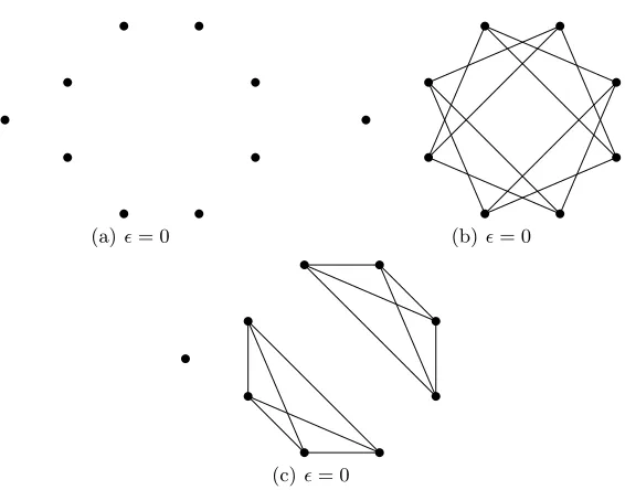
For example, consider an intersection graph onn nodes which is effectively partitioned into two sets: a set of n−1 nodes with high expansion, and a fi-nal node which is disconnected from the rest of the graph, as demonstrated in Fig. 5(b). We would find that= 0, and we would suspect that the graph is less than desirable for WSN applications.
However, particularly in a network of thousands of nodes, the disconnection of one is unlikely to be severely detrimental to the network; indeed, loss of some nodes due to poor positioning or battery failure may be expected. Knowing only that = 0 does not distinguish between the following cases:
1. the graph is completely disconnected (Fig. 5(a))
2. a single node is disconnected from the rest of the graph, which otherwise has good expansion (Fig. 5(b))
3. the disconnected graph is a union of smaller graphs, some with good expan-sion (Fig. 5(c))
If an intersection graph falls into Case 1 then it is likely that the key graph has low connectivity, ie. a low value of Pr1. However, for the same values of network size, key storage, connectivity and resilience, knowing only that = 0 in the intersection graph cannot distinguish between the Cases 2 and 3, though Case 2 is likely to be much better for WSN applications.
(a)= 0 (b)= 0
(c)= 0
Fig. 5.Distinguishing between cases where= 0
order to analyse a proposed KPS, and where possible to analyse the resulting intersection graph.
Components We note that to distinguish between the cases in Fig. 5 it is relevant to know the number ofcomponents. A component of a graph is a con-nected subgraph containing the maximal number of edges [8], that is, a subset
S of one or more vertices of the graph, where the vertices of S are connected but E(S, S) =∅. Hence Fig. 5(a) has nine components, Fig. 5(b) has two, and Fig. 5(c) has three. For WSN applications where data must be routed throughout the network, it is desirable to minimise the number of components.
Unlike finding the expansion coefficient of a graph, calculating the number of components can be done in linear time using depth-first search, as described in [15]. The global connectivity of a graph is the number of nodes in its largest component divided by the total number of nodes. We wish the global connectivity to be as close to one as possible.
Cut-edges Acut-edge (also known as abridge) is an edge whose deletion in-creases the number of components. Equivalently, an edge is a cut-edge if it is not contained in any cycle of the graph. This is illustrated in Fig. 4, where the edge (e, f) is a cut-edge.
the nodes at their endpoints, and create weak points of the network where a small fault or compromise by an adversary creates a lot of damage. Therefore, one of the reasons why expander graphs are desirable for WSNs is because they are less likely to have cut-edges:
– If > 1
b|V2|c then we know that there is no cut-edge which, if removed, would
separate the graph into two components, each of size |V2|. – If= 1
2 then it is possible that there are cut-edges which, if removed, would disconnect at most two nodes from the network
– If >1 then for all S⊂V with|S| ≤ |V2|,
|E(S, S)|>|S| ≥1 ,
and so there can be no cut-edges in the graph.
Determining whether a graph contains cut-edges can also be done by a linear time algorithm [22].
Cutpoints There is also a related notion ofcutpoints in graphs, for which we will need the following definitions from [8]. A subgraph of a graphG(V, E) is a graphGS(VS, ES) in whichVS ⊂V andES ⊂E. IfVS orES is a proper subset
(that is, VS 6=V or ES 6=E), then the subgraph is aproper subgraph ofG. If
VS orES is empty, the subgraph is called the null graph.
In a connected graphG, if there exists a proper non-null subgraphGS such
thatGS and its complement have only one nodeniin common, then the nodeni
is called acutpoint ofG. In an unconnected graph, a node is called a cutpoint if it is a cutpoint of one of its components. IfGhas no self-loops, then a cutpoint is a node whose removal increases the number of components by at least one. We see then that in Fig. 4(a), nodeseandf are cutpoints, and that graphs with good expansion will have few cutpoints.
If a graph contains no cutpoints it is said to benonseparable orbiconnected, which again is clearly desirable for an intersection graph representing a WSN. The website [1] gives examples of Java algorithms which find the nonseparable components of given graphs and can even add edges to make graphs nonsepara-ble.
These tools are just a few of the simple, effective ways to analyse an inter-section graph of a deployed WSN, and to make intelligent improvements to the structure of the graph wherever the post-deployment key management protocols allow.
7
Conclusion
with good expansion are well connected with low diameter and do not have the vulnerabilities of cut-edges and cutpoints. We have shown that the expan-sion coefficient of the product graph is not a relevant metric, but that it is the intersection graph where good expansion is desired.
In a setting where there is control over the communication graph, the expan-sion of the intersection graph should be an important consideration in the design of the key graph. If there is no control over the communication graph, then after choosing levels of network size, key storage, connectivity and resilience, the best choice of KPS is the one with the highest expansion, since it will maximise the probability of achieving good expansion in the intersection graph.
We have shown that KPSs based on expander graph constructions are able to produce key graphs with high expansion for a given network size and key storage, and use unique pairwise keys to give perfect resilience. However, many existing KPSs are able to achieve better expansion for the same key storage and network size, at the cost of lower resilience.
Finally, we have suggested that expansion is an important metric for compar-ing KPSs proposed for WSNs, and a useful parameter for analyscompar-ing intersection graphs after deployment in order to improve weak parts of the network. Deter-mining the expansion of a graph is co-NP-complete and gives only a worst-case assessment of the graph. Therefore we have proposed the use of linear time algorithms to estimate the expansion, and introduced related graph-theoretic properties which could be used to analyse the key and intersection graphs of WSNs.
References
1. Analyzing Graphs http://docs.yworks.com/yfiles/doc/developers-guide /analysis.html
2. Simon Blackburn, Keith Martin, Maura Paterson, and Douglas Stinson. Key Re-freshing in Wireless Sensor Networks. InInformation Theoretic Security, volume 5155 ofLecture Notes in Computer Science, pages 156–170. Springer Berlin / Hei-delberg, 2008.
3. M Blum, R M Karp, O Vornberger, C H Papadimitriu, and M Yannakakis. The Complexity of Testing whether a Graph is a Superconcentrator. In Information Processing Letters, 13(4-5):164–167, 1981.
4. Seyit Ahmet Camtepe and Bulent Yener. Key Distribution Mechanisms for Wire-less Sensor Networks: a Survey.Rensselaer Polytechnic Institute, Computer Science Department, Tech. Rep. TR-05-07, 2005.
5. Seyit Ahmet Camtepe, Bulent Yener, and Moti Yung. Expander Graph Based Key Distribution Mechanisms in Wireless Sensor Networks. In ICC 06, IEEE International Conference on Communications, pages 2262–2267, 2006.
6. Haowen Chan, Adrian Perrig, and Dawn Song. Random Key Predistribution Schemes for Sensor Networks. In SP ’03: Proceedings of the 2003 IEEE Sympo-sium on Security and Privacy, pages 197–213, Washington, DC, USA, 2003. IEEE Computer Society.
8. Wai-Kai Chen. Applied Graph Theory. 15(1):484, 1971.
9. Fan R. K. Chung. Spectral Graph Theory. American Mathematical Society, Cali-fornia State University, Fresno, 1994.
10. Jacek Cichon, Zbigniew Golebiewski, and Miroslaw Kutylowski. From Key Predis-tribution to Key RedisPredis-tribution. InAlgorithms for Sensor Systems, volume 6451 ofLecture Notes in Computer Science, pages 92–104. Springer Berlin / Heidelberg, 2010.
11. Paul Erd¨os and Alfr´ed R´enyi. On the Evolution of Random Graphs. In Publication of the Mathematical Institute of the Hungarian Academy of Sciences, pages 17–61, 1960.
12. Laurent Eschenauer and Virgil D Gligor. A key-management scheme for distributed sensor networks. InCCS ’02: Proceedings of the 9th ACM Conference on Computer and Communications Security, pages 41–47, New York, NY, USA, 2002. ACM. 13. Subhas Kumar Ghosh. On Optimality of Key Pre-distribution Schemes for
Dis-tributed Sensor Networks. InSecurity and Privacy in Ad-Hoc and Sensor Networks, volume 4357 ofLecture Notes in Computer Science, pages 121–135. Springer Berlin / Heidelberg, 2006.
14. Shlomo Hoory, Nathan Linial, and Avi Wigderson. Expander graphs and their applications. In Bulletin of the American Mathematical Society, 43(04):439–562, August 2006.
15. John Hopcroft and Robert Tarjan. Algorithm 447: efficient algorithms for graph manipulation. InCommun. ACM, 16(6):372–378, June 1973.
16. J. Kleinberg and R. Rubinfeld. Short Paths in Expander Graphs. Annual Sympo-sium on Foundations of Computer Science, 37:86–95, 1996.
17. Jooyoung Lee and Douglas R. Stinson. Deterministic key predistribution schemes for distributed sensor networks In Selected Areas in Cryptography, volume 3357 of
Lecture Notes in Computer Science, pages 294–307, Springer Berlin / Heidelberg, 2005.
18. Keith Martin and Maura Paterson. An Application-Oriented Framework for Wire-less Sensor Network Key Establishment. InElectronic Notes in Theoretical Com-puter Science, 192(2):31–41, 2008.
19. Maura Paterson and Douglas R. Stinson. A unified approach to combinatorial key predistribution schemes for sensor networks. Cryptology ePrint Archive, Report 201, 2011.
20. O Reingold, S Vadhan, and A Wigderson. Entropy waves, the zig-zag graph prod-uct, and new constant-degree expanders and extractors. InProceedings of the 41st Annual Symposium on Foundations of Computer Science, pages 3–28, Washington, DC, USA, 2000. IEEE Computer Society.
21. H Shafiei, A Mehdizadeh, A Khonsari, and M Ould-Khaoua. A Combinatorial Approach for Key-Distribution in Wireless Sensor Networks. InGlobal Telecom-munications Conference, 2008. IEEE GLOBECOM 2008. IEEE, pages 1–5, 2008. 22. Robert Tarjan. A Note on Finding the Bridges of a Graph. InInformation
Pro-cessing Letters, pages 160–161, 1974.
23. Yang Xiao, Venkata Krishna Rayi, Bo Sun, Xiaojiang Du, Fei Hu, and Michael Galloway. A survey of key management schemes in wireless sensor networks. In