DOI: 10.1534/genetics.103.026146
Comparative Evaluation of a New Effective Population Size Estimator Based
on Approximate Bayesian Computation
David A. Tallmon,*
,†,1Gordon Luikart* and Mark A. Beaumont
†*Laboratoire d’Ecologie Alpine, UMR Centre National de la Recherche Scientifique 5553, Universite´ Joseph Fourier, F38041 BP 53 Cedex 09, Grenoble, France and†School of Animal and Microbial Sciences,
University of Reading, Whiteknights, Reading RG6 6AJ, United Kingdom Manuscript received December 26, 2003
Accepted for publication March 1, 2004
ABSTRACT
We describe and evaluate a new estimator of the effective population size (Ne), a critical parameter in evolutionary and conservation biology. This new “SummStat”Neestimator is based upon the use of summary statistics in an approximate Bayesian computation framework to inferNe. Simulations of a Wright-Fisher population with knownNeshow that the SummStat estimator is useful across a realistic range of individuals and loci sampled, generations between samples, andNevalues. We also address the paucity of information about the relative performance ofNeestimators by comparing the SummStat estimator to two recently developed likelihood-based estimators and a traditional moment-based estimator. The SummStat estimator is the least biased of the four estimators compared. In 32 of 36 parameter combinations investigated using initial allele frequencies drawn from a Dirichlet distribution, it has the lowest bias. The relative mean square error (RMSE) of the SummStat estimator was generally intermediate to the others. All of the estimators had RMSE⬎1 when small samples (n⫽20, five loci) were collected a generation apart. In contrast, when samples were separated by three or more generations andNeⱕ50, the SummStat and likelihood-based estimators all had greatly reduced RMSE. Under the conditions simulated, SummStat confidence intervals were more conservative than the likelihood-based estimators and more likely to include trueNe. The greatest strength of the SummStat estimator is its flexible structure. This flexibility allows it to incorporate any potentially informative summary statistic from population genetic data.
T
HE effective population size (Ne) plays a central between sample periods (NeiandTajima1981;Wangrole in how a population evolves becauseNeaffects 2001;Berthieret al.2002). The most widely used
esti-the degree to which a population can respond to selec- mator is a method-of-moments estimator (moment
esti-tion, as well as its sensitivity to inbreeding effects (Crow mator), which infersNefrom the standardized variance
andKimura1970;Lande1995;Lynchet al.1995). As in allele frequencies sampled one or more generations
a result of the critical importance ofNe to evolution, apart. The change in allele frequencies (F) between
a great deal of effort has focused upon estimatingNe sample periods is an inverse function ofNe. Therefore,
accurately and precisely, and there is always a demand Necan be derived from the amount of change in allele
for efficient and usefulNeestimators. Currently, many frequencies (NeiandTajima1981;Waples1991).
How-different methods are available to inferNe, including ever, this estimator uses only the first two moments of
ones based on demographic or genetic data. These the allele frequency distribution to obtain Ne and a
methods vary in the types of information they use, their number of approximations are made in its derivation.
accuracy, and the kinds of Ne estimates they provide Several studies have noted that it is often biased high
(CrowandDenniston1988;HarrisandAllendorf (Luikartet al.1999; Wang2001;Berthieret al.2002).
1989;Waples1991;Schwartzet al.1998; Storzet al. Likelihood-based methods have been proposed to
im-2002). prove N
e estimation from temporally spaced samples
Necan be estimated from genetic data in one or more and have become more feasible because fast computers
samples (Waples 1991). Most one-sample estimators required to calculate likelihoods are more generally
use associations among alleles at different loci to infer available. In theory, these estimators should be more
Ne (Hill 1981; Vitalis and Couvet 2001). Multiple- accurate and precise than the moment estimator
be-sample methods inferNefrom temporal changes in al- cause they use more of the information provided by the
lele frequencies or the rate of coalescence of alleles
data.WilliamsonandSlatkin(1999) andAnderson
et al.(2000) developed maximum-likelihood-based esti-mators that outperform the moment estimator.
How-1Corresponding author:LECA-Ge´nomique des Population et
Biodiver-ever, these methods are computationally extremely
in-site´, UMR CNRS 5553, Universite´ Joseph Fourier, F-38041 BP 53 Cedex
09, Grenoble, France. E-mail: [email protected] tensive, so they have been evaluated only with extremely
smallNeand three or fewer alleles per locus. Recently, same summary statistics generated under simulated
con-ditions with known parameter values. Most applications
Wang (2001) used time-saving analytical
approxima-tions based on the method ofWilliamsonandSlatkin have used a rejection sampling method (Pritchardet
al.1999), in which all summary statistic values that fall
(1999) to provide a more efficient likelihoodNe
estima-tor. Unlike the latter study, which could be used only outside a given tolerance range are rejected, and only
those summary statistics that fall within the tolerance
for biallelic markers, he assumed kalleles at the same
locus could be treated as if fromkindependent, biallelic range are used to estimate the target parameters (e.g.,
Tishkoffet al.2001). The approach we use here differs loci to generate the total likelihood, with an adjustment
to take into account that there are onlyk⫺1 indepen- by using local linear regression and smooth weighting of
summary statistics and associatedNevalues falling within
dent allele frequencies. This pseudo-likelihood
estima-tor appeared to perform well relative to the full-likeli- the tolerance range.Beaumontet al.(2002) showed that
local linear regression and smooth weighting can be used hood estimators, but was compared only with three
alleles per locus and smallNe. to improve the accuracy and precision of parameter
estimation from summary statistics over that provided
More recently, Berthier et al. (2002) developed a
novel likelihood-based approach to obtainNˆefrom two by rejection sample methods.
We develop a novel Ne estimator using four simple
samples using a genealogical representation from
coa-lescent theory. Likelihoods were estimated by impor- summary statistics and local weighted regression in a
Bayesian framework. The four summary statistics are tance sampling. Markov chain Monte Carlo (MCMC)
was then used to give a Bayesian posterior distribution the divergence between samples using Weir and
Cock-erham’s (Weir 1990), the change in the number of
forNe. Using a prior distribution to set an upper limit for
Ne, which ensured convergence of the MCMC estimates, alleles from the first to second sample (⌬a), the change
in within-sample gene diversity from the first to second
Berthier et al. (2002) showed their estimator to be
superior to the moment estimator when genetic drift sample (⌬Hs;Nei1987), and the total expected
hetero-zygosity between samples (Ht;Weir1990). We evaluate
was strong. Being based on the coalescent, it is only an
approximation to the genealogy of the Wright-Fisher the performance of this summary statistics (SummStat)
estimator and compare its performance relative to three model, which assumes discrete generations. The
ap-proximation is most accurate when the sample size is existing estimators. These estimators include the
stan-dard moment estimator, which has well-known properties small relative toNeandNeis large. Because their
estima-tor relies upon Monte Carlo methods to provide the over a wide range of parameter values, and promising
likelihood estimators developed recently byBerthieret
posterior distribution of Ne, it is computationally
de-manding and has not been extensively evaluated with al.(2002) andWang(2001) that are not as well known
and have not been compared to each other. For this simulations, nor has it been compared to the
pseudo-likelihood estimator ofWang(2001). comparison we use simulated populations of knownNe
and levels of genetic variation at marker loci typical of
We develop a newNeestimator by combining simple
summary statistics from multiple genetic samples with microsatellites, the preferred marker forNeestimation
(Luikartet al. 1999). We compare the accuracy and approximate Bayesian computation and compare this
estimator to existing ones. Bayesian approaches are at- precision of these fourNeestimators, using a range of
Ne’s (20–100), numbers of loci (5 or 15), and sample
tractive because they allow for background information
to be incorporated into the model, provide posterior sizes (20 or 60) separated by a range of generations
(1–10) typical in studies of natural populations. Finally, probability distributions for parameters of interest, and
integrate out cumbersome nuisance parameters that are we illustrate the use of the methods with a real
microsa-tellite data set from an experimental population of
mos-common in population genetics data (Shoemakeret al.
1999). Potentially exact Bayesian computation (in the quito fish (Spenceret al.2000).
sense that the posterior distribution can be approxi-mated to any desired level of accuracy) using MCMC is
METHODS
often very time consuming and requires a substantial
amount of programming effort (Beaumontet al.2002). SummStat estimator:We developed anNeestimator
using the summary statistics approach developed by sev-These constraints make potentially exact Bayesian
analy-ses impractical for many applications and difficult to eral authors (FuandLi1997;Tavare´et al.1997;Weiss
andvon Haeseler1998) and modified byBeaumont
evaluate in many cases, especially for large data sets.
Thus, alternative, less time-consuming methods are de- et al. (2002) to incorporate weighted local regression
in a Bayesian context. The general method is described sirable.
The use of summary statistics has been proposed as in detail by Beaumont et al.(2002) and briefly here.
This approach is especially useful when inferences about a means to avoid the problems presented by complex
population genetics analyses (Tavare´et al.1997). This some parameter of interest, ⌽, are difficult to make
using full likelihoods. In this method, J values of ⌽i
requires the comparison of summary statistics from a
each⌽ia data set,Di, is simulated using a Wright-Fisher wherea1,iand a2,i are the estimated number of alleles
at locusi in samples 1 and 2, respectively; the change
model described below. Summary statistics,Si, are then
calculated from the data and scaled to have unit vari- in mean within-sample gene diversity from the first to
second sample,
ance. Thus, the Si and ⌽i are drawn from the joint
distributionP(S,⌽). The posterior distributionP(⌽|S⫽
S*) is the conditional distribution of⌽given the target ⌬Hˆs⫽
冢
1⫺1
L
兺
L
i⫽1
p2
1,i
冣
⫺冢
1⫺1
L
兺
L
i⫽1
p2 2,i
冣
,summary statisticsS*, calculated from the sample data.
To approximate this, the simulated candidate value⌽i
wherep2
1,iandp22,iare the squares of the estimated
fre-and associatedSiare accepted when the Euclidean
dis-quency of each allele present at locusiin the first and
tance ||Si ⫺ S*|| ⬍ g, where g defines a distance such
second samples, respectively (Nei1987); and total
ex-that a proportiondgof points closest toS* are accepted
pected heterozygosity between samples,
(Fu and Li 1997; Tavare´ et al. 1997; Pritchard et
al.1999). To improve the accuracy of the “rejection”
Hˆt⫽ 1⫺
1
L
兺
L
i⫽1
p2 i,
scheme, in the method ofBeaumontet al.(2002) each
accepted⌽iis given a weight that declines quadratically
as a function of ||Si ⫺S*|| from 1 at distance 0 to 0 at where p2i is the estimated frequency of each allele in
the combined samples (Weir1990). All estimated values
distanceg, and then weighted linear regression is used
to adjust the values of⌽i. The method fits a regression for these summary statistics also included appropriate
sample size corrections. line such that each⌽i⫽a⫹bSi⫹ei, and then, assuming
constant variance within the interval given by ||Si ⫺ It is important to note that we could have included any
summary statistics that can be calculated from standard S*|| ⬍ g, makes the adjustment⌽⬘i ⫽ a ⫹ b(S* ⫺ Si).
These⌽⬘i are then assumed to be random samples from population genetic data, but limited ourselves to four
that are straightforward to calculate, commonly used in
the posterior distributionP(S,⌽), which, depending on
how close to sufficient are the summary statistics, is itself population genetics studies, and thought to be related
to our parameter of interest,Ne, on the basis of previous
assumed to be close toP(D|⌽).
To examine our SummStat Neestimator, we created research and some preliminary simulations of our own.
The simulation model sampled from a uniform flat an individual-based, Wright-Fisher simulation model of
diploid organisms using the programming language C. prior distribution ofNebetween 4 and 400 to generate
J⫽ 50,000 values of the summary statistics. This prior
This model differs slightly from a Wright-Fisher model
in that there are two allogamous sexes and equal num- is reasonable becauseNecan fall in this range, even for
some populations with thousands of individuals, and bers of each sex. In the present case, the model was
initialized using genotypes drawn from a uniform Dir- because most applications of Ne estimators are cases
where Ne is small (Waples 1991). To test the
perfor-ichlet distribution with eight alleles per locus, but it can
also be initialized using a coalescent-based microsatellite mance of the SummStat estimator, we simulated
inde-pendent populations of knownNeand calculated
sum-distribution with any specifiedvalue or range of values.
Following the collection of the first sample ofndiploid mary statistics for each target data set sampled from
each population (see details of sampling conditions
be-individuals at timet1⫽0, a breeding population of size
Newas created and randomly mated fortgenerations, low). We used natural log of Ne in all regressions to
adjust the values of⌽i to ensure that the results were
when the second sample of n diploid individuals was
collected from progeny of adults in generationt2. Fol- robust to changes ing. Values ofNeaccepted withindg⫽
0.02, as described above, were then regarded as samples lowing the collection of the second sample, summary
statistics were estimated over theL loci sampled. This from the posterior distribution ofNe. The mode and
credible intervals of the posterior distribution of
back-sampling schedule follows plan 2 of Waples (1989).
The summary statistics consisted of a common measure transformedNevalues were calculated using the density
estimation method ofLoader(1996), implemented in
of divergence between samples, the coancestry
coeffi-cient, the statistical package R (RDevelopment Core Team
2003). The log transformation did not prevent some regression-adjusted points from projecting beyond the
ˆ ⫽ 1
L
兺
L
i⫽1
(Qi⫺qi)/(1⫺qi) ,
upper bound ofNe.
Comparison to other estimators: We compared the whereQiis the estimated probability of identity of alleles
performance of the SummStat estimator to three
exist-in a sample at locusiandqiis the estimated probability
ing two-sample Ne estimators, including a coalescent
of identity of alleles in the two samples at locusi(Weir
(TMVP;Beaumont2003, which is based on the program
1990); the mean change in the number of alleles from
TM3 inBerthieret al.2002), a moment (NeiandTajima
the first to second sample,
1981), and a pseudo-likelihood (MLNE;Wang2001)
esti-mator. The comparisons were conducted over a range
⌬aˆ⫽ 1
L
兺
L
i⫽1
(a1,i ⫺a2,i) ,
sizes (Ne⫽ 20, 50, 100), generations between samples cies are drawn from a uniform Dirichlet distribution in
(t⫽1, 3, 5, 10), sample sizes (n⫽20, 60 diploid individu- most simulation-based studies ofNeestimators,
includ-als), and numbers of loci (L⫽5, 15). Note that in some ing ours (Andersonet al.2000;Wang2001). This
corre-situations the sample size exceeded the effective size, sponds to specific assumptions about the mutation
pro-which is common when sampling natural populations cess—namely, that it is a k-allele model where each
in which the number of juvenile or adult individuals mutation occurs at rate⌰, and the probability of
muta-can greatly exceed the number of breeders (Frankham tion to any specific allele is 1/k. We investigated the
1995) and corresponds to sampling plan II of Waples robustness of our results to assumptions about the
un-(1989). Only one set of simulations with largeNe⫽100 derlying allele frequency distribution by initializing a
is included (t ⫽ 1, 3, 5, 10;n ⫽ 60; L⫽ 15), because set of simulations and priors with allele frequency data
of the long time required to run all of the models on drawn from the coalescent. For these simulations the
largeNepopulations and because most applications of Wright-Fisher population described above was used.
Ini-Neestimators are to natural populations with smallNe. tial levels of polymorphism were determined by a
ran-We ran 600 independent iterations of each combination domly selected value of⌰ ⫽5–15, and the population
of parameter values for the model comparisons. The was first sampled t
1 ⫽ 1–10 generations following a
models were compared in terms of bias and precision change in effective size to N
e ⫽ 20. We used uniform
ofNˆe, using a number of metrics: relative mean square flat priors for ⌰ and the t
1. The second sample was
error (RMSE) of the mode, median bias of the mode, collectedt
2⫽1, 3, 5, or 10 generations aftert1. In each
95th percentile of 95% confidence/credible intervals, sample,n ⫽ 60 individuals were genotyped atL ⫽ 15
and proportion of confidence/credible intervals that loci. The estimators were evaluated as described above
excluded trueNe. We also show the bootstrapped esti- on the basis of 600 iterations of each set of conditions.
mates of the standard errors of the RMSE estimates. With this slight modification we are now able to obtain
All sampled genotypes generated in our simulations the posterior distribution ofN
emarginal to both⌰and
were written to files to provide input for TMVP and t
1. This highlights the advantage of approximate
Bayes-MLNE. TMVP is an updated version of the TM3 pro- ian computation based on summary statistics, and it
gram used in Berthier et al. (2002) and provides a is straightforward to make changes in the model with
posterior distribution of Ne using a MCMC approach minimal programming effort.
with importance sampling (Beaumont2003). For the
Real data set:To further illustrate the SummStat esti-simulations used here, the size of the importance sample
mator, we estimated Ne for an experimentally
bottle-was 20, 20,000 MCMC updates were used with 10 updates
necked population reported in Spencer et al. (2000)
between estimate outputs, and anNeceiling was set at 400. and evaluated by Berthier et al. (2002), using their
The TMVPNeevaluated in this article is the mode from coalescent-based
Neestimator and the moment
estima-the posterior MCMC distribution of values (except for an
tor. The target data set was collected from a large source initial 10% of values discarded as burn-in).
population of mosquito fish (Gambusia affinis) that was
MLNE provides a pseudo-likelihoodNeas described
sampled and then experimentally reduced to eight pairs
in Wang (2001). We used an updated version of the
of founders, allowed to grow for two generations, and
program, described in Wang and Whitlock (2003),
then resampled (Spenceret al.2000). Forty individuals
which provides a ceiling forNe. We used anNeceiling
were genotyped at eight microsatellite loci in each
sam-of 400 in these simulations. MLNE also providesNefrom
ple. Although trueNeis unknown for this population,
the moment estimator of NeiandTajima(1981), but
Ne⫽16 is the hypothesized value. For this target data
no confidence intervals. Therefore, the 95% confidence
set we generated values for the same summary statistics intervals of the moment estimator are not reported and
used in our simulations:ˆ⫽0.283,⌬aˆ⫽ ⫺5.50,⌬Hˆs⫽
described here, but they have been explored previously
⫺0.096, and Hˆt ⫽ 0.708. We used the same
Wright-and their precision Wright-and bias are well known (Luikart
Fisher model described above to simulate 50,000 popu-et al.1999;Wang2001;Berthier et al.2002).
lations, with anNerandomly drawn from a uniform flat
Robustness to prior probability distribution ofNe:We
prior between 4 and 500 and initial levels of polymor-investigated the robustness of the SummStat estimator
phism determined by the coalescent with a uniform flat to changes in the prior probability distribution (using
prior for between 5 and 15. In each simulation, 40
the same metrics described above) when the lower limit
diploid individuals were sampled and genotyped at eight of the prior remained at 4 and upper limit of the prior
loci in generations 0 and 2. These genotypes were used
probability distribution for Ne was 200, 400, or 1000.
to calculate the same summary statistics calculated for
TrueNewas set to 50. Diploid individuals were sampled
the target data set, with the tolerance set at 0.02. We 1 or 3 generations apart and genotyped at 15 loci. We
report the mode and 95% credible intervals of the poste-did not directly compare the SummStat estimator to the
rior distribution from SummStat and compare them to others in these simulations. Results are based upon 600
the other estimators. The estimates from TMVP and the iterations of each set of conditions.
al.(2002; Table 3). MLNE estimates were obtained using Comparison to other estimators:The SummStat esti-mator has the lowest bias and generally performs well a ceiling of 500.
relative to the other estimators. When only 1 generation
passes between samples (t⫽1), TMVP and MLNE tend
RESULTS AND DISCUSSION
to underestimateNe, whereas the SummStat estimator
slightly overestimates it (Figure 1). In general, TMVP
Estimator performance:The SummStat estimator
pro-vides accurate and preciseNˆeacross a range of genera- shows the largest bias of the four estimators when 1–5
generations pass between sampling events. In contrast, tions between samples and numbers of individuals and
loci sampled. In general, this estimator shows a small, with 10 generations passing between sampling events,
the bias of TMVP is greatly reduced, whereas the mo-positive bias when only a single generation passes
be-tween samples (Figure 1). Only whenNe⫽50 and sam- ment estimator has the greatest bias. MLNE generally
shows the second lowest bias after the SummStat estima-pling conditions are at their worst (only 20 individuals, 5
loci, and 1 generation) did SummStat show a substantial tor, and this bias decreases with increasing generations
between samples.Wang(2001) reported a slight
posi-positive bias. The bias decreases rapidly with increases
in the number of individuals sampled, loci sampled, tive bias for MLNE that is based on the mean of theNe
estimates, rather than on the median as reported here. and generations between samples. The relative mean
square error (RMSE) of the SummStat estimator is small In fact, the distribution of Ne estimates is skewed (as
illustrated in Wang and Whitlock 2003, Figure 3),
when trueNe⫽20, but is noticeably larger whenNe⫽
50 and only 1 generation separates the samples (Figure and the mean is generally larger than the median, as
reported here. 2). There is a consistent, striking decrease in the RMSE
when the number of generations between samples in- All of the estimators generally show reduced bias and
RMSE with increasing sample sizes, loci, and genera-creases from 1 to 3, regardless of the other sampling
conditions. However, there is relatively little increase in tions between samples. The exception is the moment
estimator, which shows increasing bias with increasing accuracy and precision as the number of generations
increases from 3 to 10. generations between samples. In most cases simulated,
SummStat RMSE is intermediate to that of the other The SummStat 95% credible intervals contain true
Neconsistently and do not depart greatly from the ex- estimators, and the relative performance of the
estima-tors changes with sampling conditions. However, the
pectation of 2.5% of the trueNevalues falling above or
below the credible intervals (Table 1). There is a slight RMSE of the SummStat estimator is generally larger
than that of MLNE, which often provides the smallest
tendency to exclude true Ne from the lower credible
interval with sparse data and a single generation be- RMSE, and is consistently smaller than the RMSE of the
moment estimator. TMVP shows very small RMSE and tween samples, which probably is due to the slight
posi-tive bias of the SummStat estimator under these condi- little bias when 10 generations pass between samples.
In contrast, the moment estimator consistently has the tions noted above. In addition, the 95th percentiles of
the 95% credible intervals tend to be conservative when largest RMSE when there are 10 generations between
samples. data are sparse or drift is weak (Table 2). The SummStat
95% credible intervals narrow rapidly with increasing TMVP and MLNE tend to exclude true Nefrom the
upper 95% credible/confidence interval much more numbers of generations between samples. For the
pa-rameter combinations evaluated, a threefold increase than expected by chance (Table 1). This tendency is
most notable with TMVP, which consistently provides in the number of loci sampled provides a markedly
greater increase in precision than a threefold increase the lowest upper and lower confidence intervals. The
observed bias of the confidence intervals generally wors-in the number of wors-individuals sampled.
The SummStat estimator appears robust to changes ens with the number of loci or individuals sampled, if the
number of generations between samples is held constant. in the upper limit for the prior probability distribution
ofNe. The bias, RMSE, and lower credible interval of the In contrast, the observed downward biases of the 95%
confidence/credible intervals of TMVP and MLNE im-estimator do not change much with a fivefold change in
the upper limit of theNeprior from 200 to 1000 and true prove rapidly with increasing generations between
sam-ples. Although the 95% credible intervals of the
Summ-Ne⫽ 50 (Table 3). However, while the lower credible
interval is relatively stable, the upper credible interval Stat estimator are less likely to exclude true Neacross
the entire range of sampling conditions, the 95% confi-does appear to be sensitive to the choice of a prior when
only a single generation separates samples. For example, dence/credible intervals of the other estimators are
of-ten narrower when there are few generations between the upper credible interval more than doubled with a
fivefold increase in the upper limit of theNeprior. With samples (Table 2). Consequently, there is a fairly
consis-tent trade-off in the bias and precision of these estima-three generations between samples the upper credible
limit changed by⬍25% with a fivefold increase in the tors, especially when data are sparse,Nelarge, and few
generations pass between samples. TMVP and MLNE
upper limit of theNeprior. This limit changes less with
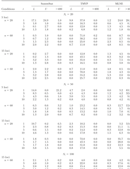
TABLE 1
Percentage of lower and upper credible/confidence limits that exclude trueNe
SummStat TMVP MLNE
Conditions t L U ⬎400 L U ⬎400 L U ⬎400
Ne⫽20 5 loci
n⫽20 1 17.1 24.9 1.0 9.8 37.8 0.0 1.2 24.0 28.5
3 1.0 1.0 0.0 0.0 16.3 0.0 0.6 4.5 0.3
5 0.1 2.7 0.0 0.0 12.8 0.0 1.3 4.5 0.0
10 1.3 1.8 0.0 0.2 6.8 0.0 1.2 1.8 0.0
n⫽60 1 0.3 1.0 0.0 0.0 71.0 0.2 0.6 8.7 0.0
3 0.7 1.2 0.0 0.0 38.2 0.0 1.0 2.7 0.0
5 1.5 2.3 0.0 0.0 25.0 0.0 2.3 0.5 0.0
10 2.0 2.2 0.0 0.7 11.0 0.0 4.8 0.5 0.0
15 loci
n⫽20 1 0.2 2.7 0.0 0.0 12.8 0.0 1.3 4.5 0.0
3 0.2 1.3 0.0 0.0 43.5 0.0 0.3 9.2 0.0
5 3.2 3.3 0.0 0.0 35.0 0.0 0.3 7.5 0.0
10 1.3 2.8 0.0 0.3 16.5 0.0 0.8 3.8 0.0
n⫽60 1 2.0 2.2 0.0 0.7 11.0 0.0 4.8 0.5 0.0
3 1.3 1.7 0.0 0.0 78.8 0.0 1.8 4.3 0.0
5 3.2 2.8 0.0 0.0 55.2 0.0 5.3 2.0 0.0
10 2.0 2.5 0.0 0.0 25.7 0.0 12.2 0.3 0.0
Ne⫽50 5 loci
n⫽20 1 14.0 0.0 21.2 4.7 2.0 0.0 0.0 3.2 83.2
3 8.3 0.5 6.0 4.5 4.3 0.0 1.2 4.2 32.0
5 4.3 0.6 1.6 3.0 3.5 0.0 1.3 4.2 9.8
10 2.2 1.3 0.2 0.8 4.0 0.0 0.8 4.2 0.8
n⫽60 1 6.3 0.6 3.2 1.0 23.2 0.0 0.3 12.7 12.0
3 3.0 1.2 0.2 0.3 14.5 0.0 0.3 5.7 0.6
5 1.8 1.8 0.0 0.5 13.2 0.0 1.0 7.0 0.2
10 1.3 2.0 0.0 0.7 8.2 0.0 1.2 3.2 0.0
15 loci
n⫽20 1 10.7 0.2 6.5 2.3 10.2 0.0 0.0 3.2 53.0
3 2.3 0.8 0.2 0.3 15.3 0.0 0.0 11.1 1.2
5 0.6 1.5 0.0 0.2 14.2 0.0 0.3 12.8 0.0
10 4.6 1.3 0.0 0.6 17.8 0.0 1.5 6.3 0.0
n⫽60 1 1.8 0.3 0.0 0.0 72.0 0.0 0.0 35.7 0.0
3 1.7 1.5 0.0 0.0 43.3 0.0 0.0 20.8 0.0
5 1.7 1.8 0.0 0.0 31.8 0.0 0.2 12.3 0.0
10 3.8 1.5 0.0 0.8 17.8 0.0 1.3 5.5 0.0
Ne⫽100 15 loci
n⫽60 1 2.1 1.3 0.2 0.8 4.0 0.0 0.8 4.2 0.8
3 4.0 1.0 0.2 0.3 22.0 0.0 0.3 17.6 0.5
5 2.0 1.2 0.0 0.0 15.4 0.0 0.0 12.0 0.0
10 1.5 1.9 0.0 0.5 13.3 0.0 0.2 9.0 0.0
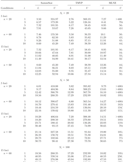
TABLE 2
Ninety-fifth percentiles of the lower and upper confidence/credible limits for theNeestimators
SummStat TMVP MLNE
Conditions t L U L U L U
Ne⫽20 5 loci
n⫽20 1 3.50 355.97 2.76 369.19 7.27 ⬎400
3 6.57 173.20 5.22 126.16 8.41 79.61
5 7.32 101.95 6.17 58.45 8.95 56.47
10 7.91 53.67 7.26 45.05 9.66 45.93
n⫽60 1 7.46 135.50 3.50 36.33 10.1 50.49
3 8.78 62.50 5.83 35.82 11.29 43.50
5 9.26 51.88 6.85 37.15 11.91 43.40
10 8.60 45.20 7.49 38.39 12.26 44.53
15 loci
n⫽20 1 7.32 101.95 6.17 58.45 8.95 56.47
3 10.66 47.64 7.81 30.00 10.97 34.42
5 11.02 40.85 8.91 31.08 11.49 33.30
10 11.49 34.99 10.41 30.17 12.54 32.70
n⫽60 1 8.60 45.20 7.49 38.39 12.26 44.53
3 11.84 36.21 8.03 23.11 13.89 29.73
5 12.03 35.00 9.35 35.47 14.54 31.50
10 12.25 32.94 10.66 27.34 15.14 32.46
Ne⫽50 5 loci
n⫽20 1 6.01 418.88 3.82 395.82 9.73 ⬎400.00
3 9.17 404.96 8.84 388.23 13.65 ⬎400.00
5 12.42 366.70 12.99 367.70 16.10 ⬎400.00
10 18.56 268.35 17.29 232.99 18.82 195.88
n⫽60 1 10.12 390.67 6.80 365.54 14.27 ⬎400.00
3 16.70 279.41 13.83 191.48 19.53 163.09
5 18.44 216.59 15.85 136.04 20.10 134.71
10 22.16 139.62 19.80 111.39 22.97 115.33
15 loci
n⫽20 1 10.28 406.64 7.20 388.48 14.51 ⬎400.00
3 18.20 298.50 16.33 279.80 19.51 193.06
5 23.71 188.41 20.02 136.26 22.03 119.83
10 30.48 93.13 27.45 74.99 30.65 79.64
n⫽60 1 21.14 227.58 11.51 91.64 19.80 105.38
3 26.33 130.72 19.51 75.30 24.81 80.33
5 28.73 102.66 23.12 72.81 27.71 77.82
10 30.73 90.41 27.38 73.70 30.65 77.81
Ne⫽100 15 loci
n⫽60 1 18.56 268.35 17.29 232.99 18.82 195.88
3 40.95 338.54 35.06 271.64 40.53 250.12
5 49.13 276.98 43.94 192.89 47.53 191.12
10 55.62 210.41 51.22 168.61 54.37 172.06
The 95th percentile of the 95% confidence/credible lower (L) and upper (U) limits of threeNeestimators is shown. See Table 1 for details.
trueNe. The SummStat estimator provides relatively con- a Dirichlet distribution to draw initial allele frequencies
also appear to be robust to changes in the underlying servative credible intervals and is less biased.
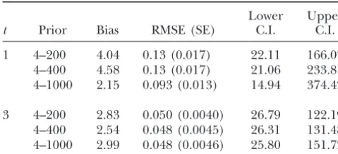
TABLE 4 TABLE 3
Robustness of SummStat estimator to changes in theNeprior Coverage of theNeestimators with initial allele frequencies drawn from the coalescent
Lower Upper
t Prior Bias RMSE (SE) C.I. C.I. SummStat TMVP MLNE
1 4–200 4.04 0.13 (0.017) 22.11 166.07 t L U L U L U
4–400 4.58 0.13 (0.017) 21.06 233.81
%Neexcluded 4–1000 2.15 0.093 (0.013) 14.94 374.42
1 8.0 0.2 0.0 98.6 0.0 93.6
3 3.2 0.6 0.0 94.3 0.0 81.0
3 4–200 2.83 0.050 (0.0040) 26.79 122.19
5 3.0 0.8 0.0 89.7 0.1 70.3
4–400 2.54 0.048 (0.0045) 26.31 131.48
10 2.3 2.0 0.0 76.8 0.3 46.8
4–1000 2.99 0.048 (0.0046) 25.80 151.72
Metrics shown are the same as those described in Figures 95th percentile of C.L.
1 and 2 and Table 1. Values are based upon 600 iterations 1 4.00 179.64 1.10 13.13 5.26 20.90 with true Ne ⫽ 50 and 15 loci from 60 diploid individuals 3 4.38 100.49 2.78 20.71 6.48 25.50 sampledt⫽1 or 3 generations apart. All prior distributions 5 4.97 75.96 3.99 22.10 7.38 26.66 are uniform flat between the values shown. C.I., confidence 10 6.39 54.75 5.73 25.00 8.57 28.64 interval.
Coverage includes the percentage of trueNevalues excluded (%Neexcluded) from the lower (L) and upper (U) confi-dence/credible limits and the 95th percentiles of the 95%
analyses. The patterns of bias and RMSE of the
estima-confidence/credible limits (95th percentile of C.L.). Values
tors are similar whether initial allele frequencies are
are based upon 600 iterations with trueNe⫽20 and 15 loci
drawn by sampling from a Dirichlet or from the coales- genotyped from 60 diploid individuals sampledtgenerations
cent. However, the tendencies of each estimator noted apart.
above appear to be accentuated. The SummStat estima-tor continued to show the lowest bias (Figure 1) as well
as a relatively large RMSE when few generations passed very accurate and precise when 10 generations pass
be-tween samples, despite the fact that it suffers from a between samples (Figure 2). TMVP and MLNE were
precise, but showed considerably strong bias. A notice- disadvantage in our comparisons in that it assumes a
coalescent model to simulate drift and a Wright-Fisher able change in the relative performance of these
estima-tors is the improved performance of the moment estima- model was assumed for our simulations. Indeed, TMVP
was very accurate in a subset of simulations using the tor in the coalescent simulations, especially with 5–10
generations between samples. The positive bias and low coalescent rather than a Wright-Fisher model to
simu-late drift (data not shown). accuracy of the moment estimator when drift is strong
have been noted elsewhere to result from the fixation Empirical data:The application of SummStat to data
collected from an experimental mosquito fish popula-of low-frequency alleles present in the first sample
(RichardsandLeberg1996; Luikartet al.1999;Wil- tion studied bySpenceret al. (2000) demonstrates its utility in an empirical setting. The SummStat point
esti-liamson and Slatkin1999; Wang 2001;Berthier et
al.2002). The improved performance here is probably mate of Ne ⫽ 8.93 falls below the hypothesized true
Ne⫽16 for this population. In contrast, the coalescent,
due to there being fewer rare alleles because the
simu-lated populations were first sampled as many as 10 gen- moment, and MLNE estimates are 21.6, 35.4, and 32.51,
respectively. More importantly, the SummStat Ne 95%
erations following the initial reduction inNe. This long
period of strong drift before drawing the first sample credible intervals contain the hypothesized trueNevalue
and are reasonably precise, whereas all of the others could decrease the number of rare alleles, thus reducing
this source of bias for the moment estimator. excluded Ne from their credible/confidence intervals
(Figure 3). In this case, only eight loci and 40 individuals The patterns seen in the 95% confidence/credible
intervals when initial allele frequencies are drawn from were sampled, which is a modest sampling effort to
expect for most natural populations. Although this is the coalescent are also similar to the patterns in
simula-tions that draw from the Dirichlet. Namely, the Summ- only a single application of the SummStat estimator,
the results are encouraging and suggest the estimator Stat credible intervals are conservative and are slightly
more likely to fall above than below trueNe(Table 4). may work well when applied to microsatellite data
sam-pled from real populations. In contrast, the confidence/credible intervals of TMVP
and MLNE tend to fall below trueNeand provide under- Other considerations:It has been suggested byWang
and Whitlock (2003) that measurement of bias and
estimates of trueNequite frequently.
TMVP provides point estimates and upper credible precision should be based on 1/(2Ne) rather than on
Ne. The relative advantages or disadvantages of different
intervals that are biased low when there are few
genera-tions between samples, and this bias has been noted point estimators and transformations can be assessed
only in a decision-theoretic framework (O’Hagan
Figure3.—Comparison of four effective popu-lation size (Ne) estimators using data from
Rich-ards and Leberg (1996) for an experimental
population of mosquito fish. Lines indicate point estimates and shaded boxes indicate 95% confi-dence/credible intervals.
1994), where a utility function can be specified forNe, summary statistic than, for example, divergence
be-tween samples. Thus, careful attention should be paid and in the absence of this we prefer to measure bias
and precision in terms ofNe. Examination of a number to choosing statistics that are likely to be informative,
as one seeks to maximize the amount of information of data sets indicates that the general patterns in the
data reported here are robust whether one examines that can be extracted from a data set while avoiding the
curse of dimensionality created by using many different estimates ofNeor 1/(2Ne).
An important choice in Bayesian inference is the summary statistics (Beaumontet al.2002). Ideally, both
the literature and simulations should be used to help method used to generate the prior probability
distribu-tion. We have found our estimator to be robust whether choose the best summary statistics for a given set of
biological conditions and sampling constraints. initial allele frequencies are drawn from the Dirichlet
or the coalescent. However, as with any Bayesian ap- Conclusions:The SummStat estimator performs well,
relative to the others, using only four summary statistics. proach, it is important to recognize that large
differ-ences between the biological conditions that gave rise It is the least biased method over the full range of
parameter values investigated, has an RMSE intermedi-to the data and the method used intermedi-to generate the prior
can affect the validity of the results. Common effects of ate to the others in most of the scenarios investigated,
and performed well when applied to a real data set. small population size, such as small departures from
Hardy-Weinberg proportions or gametic phase equilib- However, MLNE generally has the smallest RMSE of
the estimators compared, despite a negative bias and rium, should not create problems in our simulations
because the assumed model incorporates these effects tendency to exclude trueNefrom the upper confidence
intervals when few generations pass between samples. adequately. However, if the target data had been
col-lected from a population with high rates of undetected The complementary properties of MLNE (precision)
and SummStat (accuracy) suggest that it would be wise immigration, for example, and the model used to
gener-ate the priors did not incorporgener-ate this, then biological to use both to estimateNe. TMVP may be more
appro-priate when reproduction occurs continuously rather inferences could be misleading. Consequently,
research-ers should temper their interpretations with careful con- than in discrete generations.
The SummStat estimator is best viewed as a flexible
sideration of the assumptions (e.g., immigration, no
sub-structuring, neutral markers) used in creating the prior approach to Neestimation, in terms of both modeling
and choice of summary statistics, as shown by the ease probability distribution and how differences within the
biological context that created the data set of interest with which it is modified to consider a very different
prior from a Dirichlet. An advantage of the SummStat might affect their inferences.
It is also important to note that the quality of the estimator is that one can combine any potentially
infor-mative summary statistics calculated from sample data information provided by each summary statistic will vary
with sampling conditions, amounts of genetic drift, and into a single approach to Ne estimation. For example,
it could conceivably be extended beyond the allele fre-type of genetic markers. For example, if molecular
mark-ers or populations with few alleles are studied, then the quency-based information used in the present example
ral changes in allele frequencies provide estimators of population
information provided by the data (Hill1981;Waples
bottleneck size. Conserv. Biol.13:523–530.
1991). The time-saving attributes of approximate Bayes- Lynch, M., J. ConeryandR. Burger, 1995 Mutational meltdowns
in sexual populations. Evolution49:1067–1080.
ian approaches relative to exact Bayesian methods make
Nei, M., 1987 Molecular Evolutionary Genetics. Columbia University
them an appealing alternative for population genetics
Press, New York.
applications. New molecular technologies provide ever- Nei, M., andF. Tajima, 1981 Genetic drift and estimation of effective population size. Genetics98:625–640.
increasing numbers of molecular markers, which, in
O’Hagan, A., 1994 Bayesian Inference. Arnold, London.
turn, make full-likelihood calculations very time con- Pritchard, J. K., M. T. Seielstad, A. Perez-lezaunandM. W.
Feld-suming. The performance of the SummStatNeestimator man, 1999 Population growth of human Y-chromosomes: a
study of Y chromosome microsatellites. Mol. Biol. Evol.16:1791–
suggests further exploration and expansion using
approxi-1798.
mate Bayesian computation may be a fruitful means to RDevelopment Core Team, 2003 R: A Language and Environment
improve efficientNeestimation. for Statistical Computing. R Foundation for Statistical Computing,
Vienna (http://www.R-project.org).
We thank L. Excoffier, J. Wang, and R. Waples for helpful reviews Richards, C., andP. L. Leberg, 1996 Evaluation of the effects of and suggestions that improved this manuscript. We also thank J. Wang bottlenecks on changes in allele frequencies. Conserv. Biol.10: for graciously recompiling slightly altered versions of his program for us. 832–839.
Schwartz, M. K., D. A. TallmonandG. Luikart, 1998 Review This work was supported by a National Science Foundation postdoctoral
of DNA census and effective population size estimators. Anim. grant (INT 0202707) to D.A.T. and by the European Commission
Conserv.1:293–299. (Econogene contract QLK5-CT-2001-02461) to G.H.L. M.A.B. is
sup-Shoemaker, J. S., I. PainterandB. S. Weir, 1999 Bayesian statistics ported by a Natural Environment Research Council Advanced
Fellow-in genetics. Trends Genet.15:354–358.
ship. Spencer, C. C., J. E. NeigelandP. L. Leberg, 2000 Experimental evaluation of the usefulness of microsatellite DNA for detecting demographic bottlenecks. Mol. Ecol.9:1517–1528.
Storz, J. F., U. RamakrishnanandS. C. Alberts, 2002 Genetic effective size of a wild primate population: influence of current
LITERATURE CITED
and historical demography. Evolution56:817–829.
Anderson, E. C., E. G. Williamson and E. A. Thompson, Tavare´, S. J., D. J.Balding, R. C.Griffithsand P.Donnelly, 1997 2000 Monte Carlo evaluation of the likelihood forNefrom tem- Inferring coalescence times from DNA sequence data. Genetics
145:505–518. porally spaced samples. Genetics156:2109–2118.
Tishkoff, S. A., R. Varkonyi, N. Cahinhinan, S. Abbesand G. Beaumont, M. A., 2003 Estimation of population growth or decline
Argyropoulos, 2001 Haplotype diversity and linkage disequi-in genetically monitored populations. Genetics164:1139–1160.
librium at human G6PD: recent origin of alleles that confer
Beaumont, M. A., W. ZhangandD. J. Balding, 2002 Approximate
malarial resistance. Science293:455–462. Bayesian computation in population genetics. Genetics 162:
Vitalis, R., andD. Couvet, 2001 Estimation of effective population 2025–2035.
size and migration rate from one- and two-locus identity measures.
Berthier, P., M. A. Beaumont, J.-M. CornuetandG. Luikart, 2002
Genetics157:911–925. Likelihood-based estimation of the effective population size using
Wang, J., 2001 A pseudo-likelihood method for estimating effective temporal changes in allele frequencies: a genealogical approach.
population size from temporally spaced samples. Genet. Res.78:
Genetics160:741–751.
243–257.
Crow, J. F., andC. Denniston, 1988 Inbreeding and variance
effec-Wang, J., andM. C. Whitlock, 2003 Estimating effective population tive population effective numbers. Evolution42:482–495.
size and migration rates from genetic samples over space and
Crow, J. F., andM. Kimura, 1970 An Introduction to Population
Genet-time. Genetics163:429–446.
ics Theory. Harper & Row, New York.
Waples, R. S., 1989 A generalized approach for estimating effective
Frankham, R., 1995 Effective population size/adult population size
population size from temporal changes in allele frequency. Ge-ratios in wildlife: a review. Genet. Res.16:95–107.
netics121:379–391.
Fu, Y.-X., andW.-H. Li, 1997 Estimating the age of the common
Waples, R. S., 1991 Genetic methods for estimating the effective size ancestor of a sample of DNA sequences. Mol. Biol. Evol.14:
of cetacean populations, pp. 279–300 inReport of the International
195–199.
Whaling Commission, Special Issue 13, edited by A. R.Hoezel.
Harris, R. B., and F. W. Allendorf, 1989 Genetically effective
International Whaling Commission, Cambridge, UK. population size of large mammals: an assessment of estimators.
Weir, B. S., 1990 Genetic Data Analysis: Methods for Discrete Population
Conserv. Biol.3:181–191. Genetic Data.Sinauer, Sunderland, MA.
Hill, W. G., 1981 Estimation of effective population size from data Weiss, G., andA. von Haeseler, 1998 Inference of population on linkage disequilibrium. Genet. Res.38:209–216. history using a likelihood approach. Genetics149:1539–1546.
Lande, R., 1995 Mutation and conservation. Conserv. Biol.9:782– Williamson, E. G., andM. Slatkin, 1999 Using maximum likeli-791. hood to estimate population size from temporal changes in allele
Loader, C. R., 1996 Local likelihood density estimation. Ann. Stat. frequencies. Genetics152:755–761.
24:1602–1618.