Available Online atwww.ijcsmc.com
International Journal of Computer Science and Mobile Computing
A Monthly Journal of Computer Science and Information Technology
ISSN 2320–088X
IMPACT FACTOR: 6.017
IJCSMC, Vol. 7, Issue. 1, January 2018, pg.68 – 77
GLCM Based LDA for Human Face Recognition
Dr. Mohammed Sahib Mahdi Altaei
1, Dua’a Ali Kareem
21’2
College of Science, Computer Science Department, Al-Nahrain University, Baghdad, Iraq
1
[email protected]; [email protected]
ABSTRACT- Face recognition system is proposed in the present work depending on the grey level cooccurance matrix (GLCM) based linear discriminant analysis (LDA) method. The GLCM is used to extract eleven effective textural features for the face image, while the LDA is used to discriminant these faces between each other depending on the extracted features. The proposed method requires create some database models, each for specific face. These face models are used to be compared with test ones that input to the recognition procedure. The newly proposed idea is the use of features instead of image pixels in the LDA covariance matrix. The proposed face recognition method consists of two phases: enrollment and recognition. Different face samples are input to the enrollment phase in order to collect the average features of that face, and store them in a database to be comparable models for the recognition phase. The recognition phase compares the extracted features of the unknown test face with that stored in the database. The comparison indicates the similarity between the test face with the database models, which is used to make the recognition decision. The results of frequent tests showed that the used face recognition was about 96%, which ensure the efficiency of the used face recognition method.
Keywords: face recognition, LDA, GLCM.
I. Introduction
Biometric system is used for more secure alternative authentication in comparison to passwords or secured ID cards due to its reliability, which can be utilized in many specific devices designed for security. There are various techniques of biometrics that vary according to the used material, once common of them is the face recognition system that commonly used for secure entry into restricted facilities [1]. Face recognition approaches are either based on the use of images directly or the use of intermediate 3D models as Figure (2.2) shows. The first type that uses the image data are the techniques of interest, most of them depend on a representation of images that induces a vector space structure and requires dense correspondence. These approaches are called appearance-based or view-based approaches due to they represent an object in terms of several object views (raw intensity images). An image is considered as a high-dimensional vector, in which each point is represented in a high-dimensional vector space
calculating texture features of an image. For effective classification of different human faces, K-Nearest Neighbour classifier was used. The recognition rate of K-NN is 91%. While [3] used two methods for extracting the feature vectors using GLCM for face classification. The first method extracts the well-known Haralick features from the GLCM, and the second method directly uses GLCM by converting the matrix into a vector that can be used in the classification process. The results demonstrate that the second method, which uses GLCM directly, is superior to the first method that uses the feature vector containing the statistical Haralick features in both nearest neighbor and neural networks classifiers. Also [4] used the face part detection (FPD) algorithm and the newly proposed Gray Level Co-occurrence Matrix (GLCM) algorithm for extracted feature from the human facial images, Performance factors applied here are feature extraction accuracy and execution time it is observed that the proposed GLCM algorithm extracted the features more accurately with minimum execution time than FPD algorithm.
In this paper, the theoretical concepts related to the face recognition technique are concerned, in which data analysis and processing are employed. The analysis includes the ability of using statistical features to estimate comparable descriptors are useful in the recognition task. The conceptual combination of GLCM and LDA is employed in terms of features space to improve the representation of the test image for achieving more accurate face recognition results.
II. Problem Statement and Contribution
The general behavior of most satellite image classification methods is not look at the fine details or boundaries of different spectral regions; they observe the main cues those dominant fine details. Almost, these methods are implemented according to some considered restrictions that help to achieve acceptable results. The motivation we address in this paper is to overcome the problem of passing the fine details; this is carried out by using the GLCM for satellite image description. The choice of good descriptors makes the fine details to be observed by the classifier, and better classification results can be achieved.Previous studies point out to the ability of LDA to achieve a desired solution with acceptable precision, such that LDA is employed to establish a classification method is able to classify an expanded diversity range of satellite images. The contribution of present work falls in the use of GLCM based LDA to solve the problem of classifying the fine details found in satellite images. The GLCM is used to provide more accurate descriptors, while the LDA uses these descriptors to classify the target image into meaningful classified image.
III. GLCM Textural Descriptors
GLCM is one of the most popular textural analysis [11]. The key concept of this method is generating features matrix to measure the spatial relationships between pixels depending on texture information. Then, cooccurrence features are obtained from this matrix [7]. Texture is one of the important characteristics used in identifying objects of interest in an image, which reflects important information about the structural arrangement of object surfaces. The textural features based on gray-tone spatial dependencies have a general applicability in image classification. GLCM is a gray level dependency matrix that represented as a two dimensional histogram of gray levels for a pair of pixels, which are separated by a fixed spatial relationship called displacement vector d, which is defined by its radius δ and orientation θ. By considering 3Χ3 image segment with four gray-tone values: 0, 1, 2, and 3. The generalized GLCM for that image, where h(i,j) stands for number of times gray [3]. In such case, the tones i and j have been neighbors satisfying the condition stated by displacement vector d. The three fundamental pattern elements used in human interpretation of images are: spectral, textural and contextual features. Spectral features describe the average tonal variations in various bands of the visible and/or infrared portion of an electromagnetic spectrum. Textural features contain information about the spatial distribution of tonal variations within an image band. There are a number of textural features proposed by Haralick et all [11] contain information about image texture characteristics such as homogeneity, gray-tone linear dependencies, contrast, number and nature of boundaries present and the complexity of the image. Contextual features contain information derived from blocks of pictorial data surrounding the area being analyzed. Statistic energy is the first feature refers to the angular second moment that measures the textural uniformity of repeating pair of pixels. It detects disorders in textures. Energy takes maximum normalized value for less homogeneous region, and can be computed as follows:
∑ ∑ … (1)
Second feature (f2) is the entropy is a statistic measure of disorder or complexity of an image. It takes a large normalized value when the image is not texturally uniform and tends to appear as a complex texture, which is strong inversely correlated to energy. The entropy is computed by the following relation:
∑ ∑ … (2)
While, the third feature (f3) is the contrast of the image is a statistic measure for the difference between the highest and the lowest values of a contiguous set of pixels. It measures the amount of local variations present in the image, and computed by the following relation:
∑ ∑ ( ) … (3)
The fourth feature (f4) is the variance, which is statistic measure of heterogeneity and is strongly correlated to first order statistical variable such as standard deviation. Variance increases when the gray level values differ from their mean. It can be computed by the following relation:
∑ ∑ ( ) … (4)
The fifth feature (f5) is the homogeneity, which is statistic measure refers to the inverse difference moment. Larger values of f5 assigned for smaller gray tone differences in pair pixels. It is more sensitive to the presence of near diagonal elements in the GLCM. It has maximum value when all elements in the image are same. GLCM contrast and homogeneity are strong inversely correlated in terms of equivalent distribution in pixel pair population. It means homogeneity decreases if contrast increases while energy is kept constant, which can be computed as follows:
∑ ∑
( ) … (5)
The sixth feature (f6) is the correlation, which is a measure of gray tone linear dependencies in the image, which refers to the amount of correlating the pixels found in a specific region in the image. It can be computed by the following relation:
∑ ∑ ( )
… (6)
The seventh feature (f7) is the sum of average that refers to the amount of total power found in a specific region of image, which can be computed as follows:
∑ ( )
… (7)
The eighth feature (f8) is the sum of entropy that describes the total entropy of a specific region in the image, which can be computed by the following relation:
∑ ( )
{ ( )} … (8)
The ninth feature (f9) is the sum of variance is a measure describing the total variance found in a specific region of image, which can be computed by the following relation:
∑ ( ) ( )
… (9)
The tenth feature (f10) is the difference of variance that measures the amount of varying the spectral tone in terms of total colors found in a specific region of image, which can be computed by the following relation:
… (10)
The eleventh feature (f11) is the difference of entropy that describes the amount of varying the disordering in a specific region of image, which can be computed by the following relation:
∑ ( )
{ ( )} … (11)
IV. Linear Discriminant Analysis
In Face Image Based LDA Computing, the computational procedure of the LDA can be given by the following steps that use to discriminant the input face images [6]:
Step-1: Provide a training set composed of a relatively large group of subjects with diverse facial characteristics. The appropriate selection of the training set directly determines the validity of the final results. The database should contain several samples of each face image are divided into two groups, one is used in the training set and the other is used in the test set.
Step-2: For each face image, starting with the two dimensional m×n array of intensity values f(x,y), the vector expansion X m×n is constructed. The vector corresponds to the feature of the face.
Step-3: By defining all feature of the same person’s face as being in one class and the faces of different subjects as
being in different classes for all subjects in the training set, find the mean for all class and mean for class i, then the within-class and between-class scatter matrices are computed. Denote the within-class scatter matrix as Sw and the between-class scatter matrix as Sb, which are defined as follows:
∑ ∑ ( )( ) … (12)
Where, Xij is the ith samples of class j, μj is the mean of class j,
∑ ( )( ) … (13)
Where, μ represents the mean of all classes. The within-class scatter matrix represents how face images are distributed closely with classes and between-class scatter matrix describes how classes are separated from each other
[Sum13].
V. Proposed Face Recognition Method
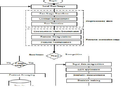
5.1 Preprocessing Stage
The preprocessing is a primary stage aims at preparing face image for highlighting the image cues that leads to estimate recognizable face features. The preprocessing stage includes two steps, they are: image transformation and contrast enhancement. The first step transforms the three color components (i.e., Red, Green, and Blue) into the intensity-chrominance components YIQ, in which only the intensity component (i.e., Y) is used in the next step:
(1),[ 11]
Where, G is the intensity component of the colored image f, while fR, fG, and fB are the color components that corresponding to the red, green, and blue bands of the image. The resulted intensity image will contains all the image cue that carried by the three color components of the face image along the visible spectrum, also the intensity image will includes all the image features that may be useful for face recognition task. The second step includes using linear fitting model to improve the contrast of the face image. By assuming that the measured minimum and maximum values of the spectral intensity image G are Gmin and Gmax frequently, and the intended minimum and maximum values of enhanced intensity image E are Emin and Emax frequently, then the enhanced image E is related to the spectral intensity image G by the following linear relationship:
(2)
Where, a and b are the coefficients of the linear fitting model between G and E. the substitution of both Gmin and Gmax that measured from the G image and the known values of Emin and Emax in eq.(3), one can gets the following two relations that containing just two unknowns a and b:
(3)
(4)
The use of equations (3 and 4) as a set of two equations with two variables enables to estimate the two unknown variable values of the linear fitting coefficients a and b by the substitution as follows:
( ) ( ) (5)
( ) ( ) … (6)
The determination of both linear fitting coefficients a and b gives the ability to compute all the pixels of the enhanced image according to eq.(2).
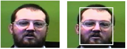
Then, the enhanced image is processed to determine just the face area in the image. The pre-established tool of Viola Jones in Matlab is used to detect the face in the image. In such process, a rectangular frame is drawn to be enclose the face appear in the image. It is easily to record the locations of the start (xs,ys) and end (xe,ye) points of that frame. These coordinates are input with the face image to the proposed face recognition method in order to isolate regions that do not belong to the determined face region. Such that, only the face region that extended between the two start and end points is deal with in the next stage.
5.2 Features Extraction
(7)
The second step includes computing the ten textural features given in equation (1-11), the computations of these equations depend on the accuracy of determining the probability P of appearing each pixel in the enhanced image. The different distribution of spectral intensity in each face image of different identity produces different features and leads to different probable spectral distribution of pixels at the image space. Different location of pixels between different face images is almost leading to different textural features belong to different face images, whereas it is normally to find the textural features are similar for same face image even with different samples. In general, the computed features are stored in features vector V of length is equal to the number of features (NF), which is split into NS NI sub vectors, each refers to features of one sample in the dataset.
The third step includes normalizing the computed features. Due to the used textural features belong to different conceptual basis; the equations of their computations are also different. This cause to produce a result is ling in different numerical range according to each feature. The use of same computed feature value may cause to bias the recognition decision into some features of great values, whereas the activity of the low valued features will be relatively lower. Therefore, it should be equalized the contribution of all the used features in producing the recognition decision. This is can be carried out by normalizing features values to be within the range from -1 to 1, this require to find out the maximum and minimum values of a jth feature Vj for all used samples in the dataset, and then use the following relationship to normalize this feature.
(
)
( ) (8)
Where, j is pointer refers to the feature serial in the features vector, Ni refers to the ith normalized feature in the features vector.
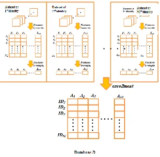
5.3 Enrollment Phase
The enrollment phase is responsible on storing the face image features in the database with a specific format. In order to establish more confident recognition, the features averaging concept is used. The average of features A is a vector of length NF, in which NS set of face image samples belong to same identity are input to estimates their features and then the average of each feature is stored in A with same index of that feature. The collection of all averaging feature of NI identities are stored in D, which is a database represented by a two dimensional array of size NF NI, Figure (2) shows the process features averaging that applied on the dataset image to create the database array D.
Fig (2) Enrollment phase workflow.
5.4 Recognition Phase
recognition scores that come from the estimated similarities are dispersed between other samples, and there is no highly score attended. There is three interested stages are adopted to make accurate recognition decision. Data composition is the first stage that aims to prepare the entry data of the adopted LDA method, in which the recognition face deals with the features vector of unknown input image and that of the face samples found in database array D. It is firstly takes the contents of D and stored it in a newly created array X, which is the LDA input data array. The size of X array is same as D with additional last column represents the features vector of the input unknown face image, i.e. NF NI+1. While, the second stage is the implementation of LDA on the prepared database. The use of features vector instead of pixel values is the newly suggested idea, where the features vector is arranged in one column of face image when constituting the input data of the LDA. Therefore, LDA algorithm is applied on the features array X to estimate the relational vector R that contains NI+1 elements, each represents the relation of feature of same index with the corresponding features in the database. whereas the third stage is concerned with estimating the percent of similarities between the query face and the samples of the database, and the result will be a similarity percentage indicates the a unique recognition decision. The similarity measure (Si) can be computed by the difference between the last value of R (i.e. RNI+1) and its previous values as follows:
[ ∑| | |
|
] (9)
In such case, Si gives the amount of similarity between the last element in the vector R that belongs to the input unknown face image and other elements of the vector R that belong to known identities stored in the database. The recognition decision depends refers to database identity of the most similarity percent.
VI. Result and Discussion
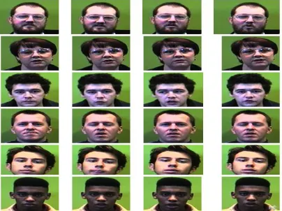
The used dataset contains different samples of same face are used for training and testing the recognition performance of the proposed method. This dataset is downloaded from CASIA web site that provides huge database of images, each is collected at specific situations for a specific subject. There are 100 face in total (NI=100) are included in the dataset, each of which is saved in colored JPEG file format, they are captured under visible illumination with spatial resolution 256*256. There are about 10 sample images are available for each face in the collected dataset, the enrolled database is depends on using only five samples (NS=5) for each face, while the remaining five samples are used for testing the proposed method. Figure (4) shows some samples of the used CASIA face dataset.
Fig (4) Some image samples for different faces in the used dataset.
Fig (5) Results of preprocessing stage applied on sample face image.
Fig (6) Result of face detection using Viola Jones method.
Frequent tests showed there are a valued stability is shown in the behavior of features set for same face image with different image samples, and fewer irregularities are shown in the behavior of each feature that belong to different sample of same face image. The stable behavior of the normalized extracted features encourages adopting the average behavior of each recognizable feature to be static model in the database. It is shown that there are some differences between the average behavior and the behaviors of its corresponding feature, this refers to that the average is almost same as features but not identical. Table (1) presents the recognition scores for ten runs, each for one sample from that found in the database. The rows in the table contains ten test samples of input face images from that used to establish the database, while the columns represent the corresponding classes that its average features are recorded in the database. It is shown that the scores lies on the diagonal is high in comparison with others, these diagonal scores describe the similarity between the input image and the samples of the database of same class. This indicates the successful of the proposed method to recognize unknown faces of such used dataset. In spite of high similarity score are resulted between two samples belong to same class, there are some high similarity scores in one run are pointed to wrong class, but it is still these wrong similarities are less than the true one. Therefore, false recognition decisions can happen with the use of huge dataset.
Table (1) Resulted recognition scores of ten successful samples.
performance accuracy. The EER is the average value of the two types of errors: FRR and FAR. The performance evaluation of the recognition is tested on five face image samples for each class to find the performance accuracy against the EER where the FAR and FRR are approximately equal in the ROC curve. Table (2) lists the computed average error values of ten test run for the five recognition samples against their FRR and FAR ratios, Figure (7) shows the behavior of FRR and FAR that given in Table (2). It is shown that the best operating point is occurred when the FAR and FRR are approximately equal at EER of about 3.274% that make the performance accuracy to be 96.725%.
Table (2) Resulted average error of the recognition test.
Fig (7) ROC curve of FRR and FAR for the recognition process.
VII. Conclusions
It is concluded that the high recognition score proves that the textural features are good descriptor for face recognition, and the behaviors of the textural features were monotonic with the variation of dataset size, and the use of more samples does not change the performance of the proposed method. Sharp image cues are very useful to describe the face in terms of numerical features. There is not sensitivity to the color, but to the grey variations of the face details. There are some stability is shown in the behavior of features set for same face image with different image samples. The false recognition decisions can happen with the use of huge dataset. The best operating point of the face recognition tests was occurred when the FAR and FRR are approximately equal at an acceptable rate of EER that make the performance to be more accurate.
0 0.5 1 1.5 2 2.5 3
1 2 3 4 5 6 7 8 9 10
Err
o
r
R
at
e
Number of tests
FRR
REFERENCES
[1] Milman, 2011 , “Techniques and Methods of Identification”
[2] Matthew Turk and Alex Pentland, (1998). Eigenfaces for Recognition, Journal of Cognitive Neuroscience, 3(1).
[3] John Wiley & Sons “Information Security Principles And Practice” San Jose State University
[4] Divyarajsinh N. Parmar, Brijesh B. Mehta 2013 “Face Recognition Methods & Applications” Int.J.Computer Technology & Applications,Vol 4.
[5] Guo-Dong Guo, Hong-Jiang Zhang, and Stan Z. Li, 2001 IEEE ,“Pairwise Face Recognition”
[6] Juwei Lu, Konstantinos N. Plataniotis,and Anastasios N. Venetsanopoulos, 2003,” Face Recognition Using Kernel Direct Discriminant Analysis Algorithms” IEEE TRANSACTIONS ON NEURAL NETWORKS, 14(1). [7] Suman Kumar Bhattacharyya And Kumar Rahul, 2013, “Face Recognition By Linear Discriminant Analysis” International Journal Of Communication Network Security, 2(2).
[8] Matthew Turk and Alex Pentland, 1998 “Eigenfaces for Recognition” Journal of Cognitive Neuroscience, 3(1). [9] Marian Stewart Bartletta, H. Martin and T
[10] Peter N. Belhumeur Joao P. Hespanha and David J. Kriegman,(1997). Eigen faces Vs. Fisher faces: Recognition Using Class Speci_C Linear Projection, IEE Trans. On Pami.
[11] R.E. Haralick, K. Shanmugam and I. Dinstein, (1973). Textural Features for Image Classification, IEEE