ABSTRACT
XIA, HENG. Energy Consumption in UWB-based Wireless Sensor Networks: A Cross Layer Analysis. (Under the direction of Dr. Arne A. Nilsson.)
c
Copyright 2011 by Heng Xia
Energy Consumption in UWB-based Wireless Sensor Networks: A Cross Layer Analysis
by Heng Xia
A dissertation submitted to the Graduate Faculty of North Carolina State University
in partial fulfillment of the requirements for the Degree of
Doctor of Philosophy
Computer Engineering
Raleigh, North Carolina
2011
APPROVED BY:
Dr. Michael Devetsikiotis Dr. Harry Perros
Dr. Wenye Wang Dr. Arne A. Nilsson
DEDICATION
To my parents Fuen Xia and Guiying Wang My dear wife Yaping Mu
BIOGRAPHY
ACKNOWLEDGEMENTS
I would like to thank all those who made it possible for me to complete this dissertation. My deepest gratitude goes first and foremost to my advisor Dr. Arne A. Nilsson. This dissertation work would not have been done without his consistent guidance and end-less help. Besides, I am so appreciative for his kindness, patience, encouragement and financial support in the past few years.
I also owe a special thanks to Dr. Wenye Wang, Dr. Michael Devetsikiotis, Dr. Harry Perros and Dr. Mihail Sichitiu. I am very thankful for their invaluable comments and critical suggestions to help me achieve a successful doctoral study.
TABLE OF CONTENTS
List of Tables . . . vii
List of Figures . . . viii
Chapter 1 Introduction . . . 1
1.1 Background . . . 2
1.2 Motivation and Objective . . . 2
1.3 Organization of the Dissertation . . . 5
Chapter 2 Related Work on Energy Consumption in Different Layers . 6 2.1 Energy Consumption in the Physical Layer . . . 6
2.2 Energy Consumption in the Data Link Layer . . . 7
2.3 Energy Consumption in the Network Layer . . . 10
2.4 Energy Consumption in the Transport Layer . . . 13
2.5 Energy Consumption in the Application Layer . . . 15
2.6 Energy Consumption at a Cross-layer View . . . 18
Chapter 3 Joint Effects of the Physical and MAC Layers on Energy Consumption of UWB-based WSNs . . . 23
3.1 Network Overview . . . 23
3.1.1 Physical Layer . . . 23
3.1.2 MAC Layer . . . 26
3.2 Energy Consumption Model of the Physical and MAC layers . . . 29
3.2.1 Energy Consumption Components . . . 29
3.2.2 State Duration and Energy Consumption . . . 29
3.2.3 Transmission Probability . . . 34
3.2.4 Closed-Form Expression of the Energy Consumption Model . . . . 39
3.3 Numerical Results . . . 41
Chapter 4 Joint Effects of the Physical and Network Layers on Energy Consumption of UWB-based WSNs . . . 46
4.1 Network Overview . . . 46
4.1.1 Network Layer . . . 46
4.1.2 Energy Consumption Model . . . 50
4.2 Energy Efficient Routing Stratergies . . . 52
4.2.1 Energy Efficient Selection of MPRs . . . 52
4.2.2 Control Messages in the OLSR extension . . . 53
4.2.3 Performance Evaluation . . . 54
4.2.5 Metrics Used in Energy Efficient Routing . . . 58
4.3 Energy Consumption Model of the Network Layer . . . 61
4.3.1 Our Radio Model . . . 61
4.3.2 Closed-Form Expression of the Energy Consumption Model . . . . 62
4.3.3 Numerical Results and Energy Analysis of Routing Protocols . . . 65
Chapter 5 Joint Effects of the Physical, MAC and Network Layers on Energy Consumption of UWB-based WSNs . . . 76
5.1 Energy Consumption Analysis of Physical, MAC and Network Layers . . 76
5.2 Closed-Form Expression of the Energy Consumption for Direct Commu-nication . . . 78
5.3 Closed-Form Expression of the Energy Consumption for Direct Commu-nication . . . 80
Chapter 6 Numerical and Simulation Results . . . 83
6.1 Assumptions and Parameters . . . 83
6.2 Numerical and Simulation Results . . . 84
6.2.1 Effects of Number of Nodes . . . 84
6.2.2 Effects of Number of Channels . . . 87
6.2.3 Effects of Amplifier Power Density . . . 97
6.2.4 Effects of Packet Body Size . . . 102
6.2.5 Effects of Minimum Contention Window Size . . . 107
Chapter 7 Conclusions and Future Works . . . 112
7.1 Conclusions . . . 112
7.2 Future Works . . . 114
LIST OF TABLES
Table 3.1 MB-OFDM and DS-UWB System Parameters. . . 26
Table 3.2 Timing Related Parameters for MB-OFDM. . . 30
Table 3.3 Timing Related Parameters for DS-UWB. . . 30
Table 3.4 System Parameters Used to Obtain Results. . . 42
Table 3.5 System Variables Used to Obtain Results. . . 42
Table 4.1 Power Value in Each Radio State. . . 51
Table 4.2 Utilized techniques and drawbacks of energy-aware routing and maximum lifetime routing. . . 57
Table 4.3 Comparison of several routing protocols for sensor networks. . . . 60
Table 4.4 UWB Radio Parameters. . . 62
Table 4.5 Variables Given Fixed Values in Our Simulation. . . 66
Table 4.6 Ranges of Variables Values in Our Simulation. . . 66
Table 6.1 Variables Contained in the Closed-Form Expression of the Energy Consumption. . . 83
Table 6.2 Parameters Contained in the Closed-Form Expression of the Energy Consumption. . . 86
LIST OF FIGURES
Figure 1.1 Protocol Stack for UWB Wireless Sensor Networks. . . 3
Figure 2.1 IEEE 802.11 Power Save Mechanism. . . 12 Figure 2.2 State transition diagram for power management modes enhanced
with IEEE 802.11 physical states. . . 21
Figure 3.1 Example of TF coding for an MB-OFDM system. . . 25 Figure 3.2 Process of Channel Negotiation and Data Exchange in MMAC. . 28 Figure 3.3 Data Transmission Sequence. . . 31 Figure 3.4 Operation of IEEE 802.11 DCF. . . 32 Figure 3.5 Markov Chain model for the back-off window size. . . 35 Figure 3.6 Energy consumption for MB-OFDM based WSN, given N=5, c=4,
W=15. . . 42 Figure 3.7 energy consumption for DS-UWB based WSN, given N=5, c=4,
W=15. . . 43 Figure 3.8 energy consumption for MB-OFDM based WSN, given m=4, c=4,
W=15. . . 44 Figure 3.9 energy consumption for DS-UWB based WSN, given m=4, c=4,
W=15. . . 45
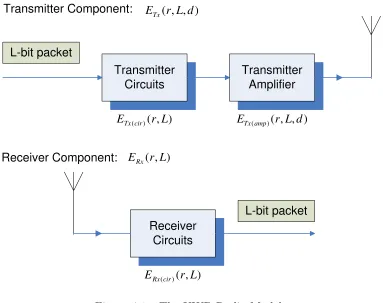
Figure 4.1 The UWB Radio Model. . . 61 Figure 4.2 100-node Uniformly Distributed Sensor Network. . . 64 Figure 4.3 Energy Consumption of Direct Communication for MB-OFDM
UWB, given n=100, L=1000 bits, r=200Mbps, Pcir = 75µW and
Iamp=1mW. . . 67
Figure 4.4 Energy Consumption of Minimum Energy Routing for MB-OFDM UWB, given n=100, L=1000 bits, r=200Mbps, Pcir = 75µW and
Iamp=1mW. . . 68
Figure 4.5 Energy Consumption of Direct Communication for DS-UWB, given n=100, L=1000 bits, r=1.3Gbps, Pcir = 75µW and Iamp=1mW. . 69
Figure 4.6 Energy Consumption of Minimum Energy Routing for DS-UWB, givenn=100,L=1000 bits,r=1.3Gbps,Pcir= 75µW andIamp=1mW. 70
Figure 4.7 Energy Consumption of Direct Communication and MTE Rout-ing, for MB-OFDM UWB and DS-UWB, givenn=100 andL=1000 bits. . . 71 Figure 4.8 Energy Consumption of Direct Communication and MTE
Figure 4.9 Energy Consumption of Direct Communication and MTE
Rout-ing, for MB-OFDM UWB and DS-UWB, givenn=100 andIamp=1mW. 73
Figure 4.10 Number of Alive Nodes, given n=100,Iamp=1mW andL=1000 bits. 74
Figure 4.11 Average Number of Neighbors for Each Node, givenn=100,Iamp=1mW
and L=1000 bits. . . 75
Figure 6.1 Ann-node random wireless sensor network. . . 85 Figure 6.2 Energy Consumption of Direct Communication for MB-OFDM
UWB and DS-UWB, withc=8,W=15,Iamp=1mW/m2andLbody=1024
bytes. . . 88 Figure 6.3 Sensor Throughput of Direct Communication for MB-OFDM UWB
and DS-UWB, with c=8, W=15, Iamp=1mW/m2 and Lbody=1024
bytes. . . 89 Figure 6.4 Energy Consumption of MTE Routing for MB-OFDM UWB and
DS-UWB, with c=8, W=15, Iamp=1mW/m2 and Lbody=1024 bytes. 90
Figure 6.5 Sensor Throughput of MTE Routing for MB-OFDM UWB and DS-UWB, with c=8, W=15, Iamp=1mW/m2 and Lbody=1024 bytes. 91
Figure 6.6 Energy Consumption of Direct Communication for MB-OFDM UWB and DS-UWB, withn=50,W=15,Iamp=1mW/m2andLbody=1024
bytes. . . 93 Figure 6.7 Sensor Throughput of Direct Communication for MB-OFDM UWB
and DS-UWB, withn=50, W=15,Iamp=1mW/m2 andLbody=1024
bytes. . . 94 Figure 6.8 Energy Consumption of MTE Routing for MB-OFDM UWB and
DS-UWB, withn=50,W=15,Iamp=1mW/m2 and Lbody=1024 bytes. 95
Figure 6.9 Sensor Throughput of MTE Routing for MB-OFDM UWB and DS-UWB, withn=50,W=15,Iamp=1mW/m2 and Lbody=1024 bytes. 96
Figure 6.10 Energy Consumption of Direct Communication for MB-OFDM UWB and DS-UWB, withn=50, W=15, c=8 and Lbody=1024 bytes. 98
Figure 6.11 Sensor Throughput of Direct Communication for MB-OFDM UWB and DS-UWB, withn=50, W=15, c=8 and Lbody=1024 bytes. . . 99
Figure 6.12 Energy Consumption of MTE Routing for MB-OFDM UWB and DS-UWB, with n=50, W=15,c=8 andLbody=1024 bytes. . . 100
Figure 6.13 Sensor Throughput of MTE Routing for MB-OFDM UWB and DS-UWB, with n=50, W=15,c=8 andLbody=1024 bytes. . . 101
Figure 6.14 Energy Consumption of Direct Communication for MB-OFDM UWB and DS-UWB, with n=50, W=15, c=8 andIamp=1mW/m2. 103
Figure 6.15 Sensor Throughput of Direct Communication for MB-OFDM UWB and DS-UWB, withn=50, W=15, c=8 and Iamp=1mW/m2. . . . 104
Figure 6.17 Sensor Throughput of MTE Routing for MB-OFDM UWB and DS-UWB, with n=50, W=15,c=8 andIamp=1mW/m2. . . 106
Figure 6.18 Energy Consumption of Direct Communication for MB-OFDM UWB and DS-UWB, withn=50,c=8,Iamp=1mW/m2andLbody=1024
bytes. . . 108 Figure 6.19 Sensor Throughput of Direct Communication for MB-OFDM UWB
and DS-UWB, with n=50, c=8, Iamp=1mW/m2 and Lbody=1024
bytes. . . 109 Figure 6.20 Energy Consumption of MTE Routing for MB-OFDM UWB and
DS-UWB, with n=50, c=8, Iamp=1mW/m2 and Lbody=1024 bytes. 110
Chapter 1
Introduction
In recent years, technology advances have made the deployment of tiny, cost, low-power devices, which are capable of sensing, processing, and communicating, a reality. These devices, called sensor nodes, when coordinate with each other, can compose a wireless sensor network (WSN) with the ability of measuring the physical environment in great detail. Due to its significant feature, such as dense distribution, flexible deployment, and local calculation, WSN has a wide range of applications in medical care, business and military. For example, in military the WSN can be used to monitor vehicular traffic and track the position of the enemy; in medical care, sensors can also be deployed to monitor patients or even implanted in the human body to detect health problems. Other applications include product quality monitoring, disaster areas monitoring, and inventory tracking, etc.
1.1
Background
The nodes in the WSN are micro-electronic devices, and like any other electronic devices, they have to be powered. Usually it is not an option to use a power cable for the nodes since that constrains the advantage of wireless communications. Hence the nodes can only be equipped with a limited energy source (e.g. a battery of less than 0.5 Ah, 1.5 V). In some extreme application scenarios, replacement of batteries might be impossible or undesirable. The node’s lifetime, therefore, shows a strong dependence on the battery lifetime. In a WSN, each node plays a dual role of data originator and data router. The malfunction of a few nodes can cause significant topological changes and might require rerouting of packets and reorganization of the network. Therefore, energy conservation takes on additional importance. It is for these reasons that researchers are currently focusing on the design of power-aware protocols and algorithms for WSNs. The main task of a node in a WSN is to detect events, perform simple local data processing, and then transmit the data. Energy consumption can hence be divided into three domains:
sensing, communicating, and data processing.
UWB is a novel radio technology that can be used for short-range high-bandwidth communications by using a large portion of the radio spectrum in a way that doesn’t interfere with other more traditional “narrow band” communications. It has been the focus of a lot of interest in recent years [12, 27, 66, 95, 108, 109, 117]. While physical layer technologies on UWB communications have been developed to some extent [66], medium access control (MAC) and higher layer technologies that enable the use of UWB in WSNs are yet to mature.
1.2
Motivation and Objective
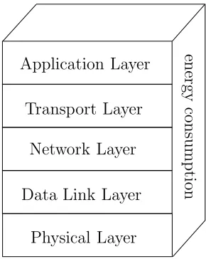
physical layer, data link layer, network layer, transport layer, and application layer, as illustrated in Figure 1.1. The physical layer is designed to address the needs of robust modulation, transmission, and reception of the data bits. In our work UWB technology is adopted in this layer. Since the environment is noisy and the nodes can be mobile, the data link layer must be able to minimize collision with neighbors’ broadcasts. The net-work layer takes care of routing the data provided by the transport layer. The transport layer helps to regulate the flow of data so that slow receivers are not swamped by fast senders. Depending on the tasks of the network, different types of application software can be built and used on the application layer. [3]
Application Layer
Transport Layer
Network Layer
Data Link Layer
Physical Layer
en
er
gy
co
n
su
m
p
tio
n
Figure 1.1: Protocol Stack for UWB Wireless Sensor Networks.
based WSN has not been thoroughly researched. [16, 81]
Given the advantages and drawbacks of the previous work in the literature, our work will focus on the cross-layer analysis of the energy consumption in UWB-based WSNs. In order to perform our analysis, we will propose an overview of the network architecture used for the WSN. It is assumed there are five layers in the protocol stack: physical layer, data link layer, network layer, transport layer, and application layer. Considering that the energy is consumed by the operations of each single layer, we will conduct our analysis based on the joint effect of different layers, more specifically the physical layer, the MAC layer, and the network layer. In order to do this, we first examine the unique characteristics of each layer of the UWB-based WSN.
In the physical layer, we will discuss the radio technology of UWB which can be divided into two different branches: Band Orthogonal Frequency Division Multi-plexing (MB-OFDM) UWB [7–9, 44], and Direct Sequence (DS)-UWB [34, 35]. In the former two or more frequency bands are employed, while in the latter only one single band is employed. Their difference is significant and therefore their way of consuming power is of big difference too. For comparison purpose, we will give the energy consump-tion analysis on both technologies. We will define the power needed for transmitting, receiving and idling states of a node.
In the MAC layer, we will discuss the multi-channel MAC protocols, with the emphasis on MMAC [92]. In MMAC, a special data structure called Preferable Channel List (PCL) is introduced in the channel selection procedure. The preferred channel for the data transmission is selected based on its priority status. At the same time, two new packet types, ATIM-ACK and ATIM-RES are introduced during the ATIM window for channel negotiation. A Markov chain is used to model the back-off window size in the MAC layer. We will propose the transmission probability and retransmission probability to derive the probabilities of five possible events for the data transmission in the MAC layer. With the power defined for transmitting, receiving and idling states, we will derive the energy consumptions of each of the above events. We will then derive the closed-form expression of the energy consumption.
transmitting and receiving power are reduced accordingly. But for every single data packet more nodes are involved in the transmission. Therefore it remains a doubt if the MTE protocol really consumes less energy than direct communication. To explore this problem we will derive the energy consumption model based on the MTE protocol and the UWB radio parameters. After that we will derive the closed-form expression of the energy consumption based on the UWB technologies, the MMAC and the MTE protocols.
Both numerical and simulation results will be presented for evaluation. By comparing the energy consumption with different UWB technologies, MAC parameters, with and without MTE routing, we will give our observations and explanations.
1.3
Organization of the Dissertation
Chapter 2
Related Work on Energy
Consumption in Different Layers
In this chapter we will review the existing literature regarding to energy consumption analysis and energy conservation algorithms in different layers of the WSN.
2.1
Energy Consumption in the Physical Layer
The physical layer is responsible for frequency selection, carrier frequency generation, signal detection, modulation, and data encryption. Thus, simple and low-power modu-lation schemes need to be developed for WSNs. Tiny, low-power, low-cost transceiver, sensing, and processing units need to be designed. Power-efficient hardware management strategies are also essential.
The UWB technology has the potential to enable low-energy consumption, high data rate communications within tens of meters, characteristics that make it an ideal choice for WSNs. [43]
UWB signals have been used for several decades in the radar community. Recently, the US Federal Communications Commission (FCC) Notice of Inquiry in 1998 and the First Report and Order in 2002 [19] inspired a renewed flourish of research and development efforts in both academy and industry due to the characteristics of UWB that make it a viable candidate for wireless communications in dense multi-path environments.
using spectrum occupied by existing radio services without causing interference, thereby permitting scarce spectrum resources to be used more efficiently. Instead of dividing the spectrum into distinct bands that are then allocated to specific services, UWB devices are allowed to operate overlaid and thus interfere with existing services, at a low enough power level that existing services would not experience performance degradation. The First Report and Order by the FCC includes standards designed to ensure that existing and planned radio services, particularly safety services, are adequately protected.
There exist two main variants of UWB. The first, known as Direct Sequence UWB (DS-UWB) [34, 35], is proposed by the IEEE P802.15 Working Group. It employs direct sequence spreading of binary phase shift keying (BPSK) and quaternary bi-orthogonal keying (4-BOK) UWB pulses. DS-UWB supports two independent bands of operation. The lower band occupies the spectrum from 3.1 GHz to 4.85 GHz and the upper band occupies the spectrum from 6.2 GHz to 9.7 GHz.
A different approach, known as Multi-Carrier UWB (MC-UWB), uses multiple si-multaneous carriers, and is usually based on Orthogonal Frequency Division Multiplex-ing (OFDM) [7–9, 44], referred to as Multi-Band OFDM UWB (MB-OFDM UWB). MB-OFDM UWB is particularly well suited for avoiding interference because its carrier frequencies can be precisely chosen to avoid narrowband interference to or from narrow-band systems. However, implementing a MB-OFDM UWB front-end power amplifier can be challenging due to the continuous variations in power over a very wide bandwidth. Moreover, when OFDM is used, high-speed FFT processing is necessary, which requires significant processing power and leads to complex transceivers.
2.2
Energy Consumption in the Data Link Layer
The data link layer is responsible for the multiplexing of data streams, data frame de-tection, medium access and error control. It ensures reliable point and point-to-multipoint connections in a WSN.
layer in the network protocol stack.
MAC protocols have been extensively studied in traditional areas of wireless voice and data communications. Time division multiple access (TDMA), frequency division multiple access (FDMA) and code division multiple access (CDMA) are MAC protocols that are widely used in modern cellular communication systems [80]. Their basic idea is to avoid interference by scheduling nodes onto different sub-channels that are divided either by time, frequency or orthogonal codes. Since these sub-channels do not interfere with each other, MAC protocols in this group are largely collision-free. We refer to them as scheduled protocols.
Another class of MAC protocols is based on contention. Rather than pre-allocate transmissions, nodes compete for a shared channel, resulting in probabilistic coordina-tion. Collision happens during the contention procedure in such systems. Classical examples of contention-based MAC protocols include ALOHA [1] and carrier sense mul-tiple access (CSMA) [56]. In ALOHA, a node simply transmits a packet when it is generated (pure ALOHA) or at the next available slot (slotted ALOHA). Packets that collide are discarded and will be retransmitted later. In CSMA, a node listens to the channel before transmitting. If it detects a busy channel, it delays access and retries later. The CSMA protocol has been widely studied and extended; today it is the basis of several widely-used standards including IEEE 802.11 [72]. Sensor networks differ from traditional wireless voice or data networks in several ways. First of all, most nodes in sensor networks are likely to be battery powered, and it is often very difficult to change batteries for all the nodes. Second, nodes are often deployed in an ad hoc fashion rather than with careful pre-planning; they must then organize themselves into a communica-tion network. Third, many applicacommunica-tions employ large numbers of nodes, and node density will vary in different places and times, with both sparse networks and nodes with many neighbors. Finally, most traffic in the network is triggered by sensing events, and it can be extremely bursty. All these characteristics suggest that traditional MAC protocols are not suitable for wireless sensor networks without modifications.
reduced compared with CSMA-based MAC protocols. TRAMA [79] is a traffic-adaptive TDMA-based protocol in which each node calculates the priorities of the nodes within two hops using a hash function for slot reservation. However, TRAMA still has its own problems. Firstly, the overhead in slot reservation is costly especially under low traffic. The channel utilization deteriorates under hotspot traffic, in which communication be-tween some nodes in a network is high. Furthermore, the duration of active period in random access for slot reservation is fixed and not traffic-adaptive.
Regardless of which type of MAC scheme is used for WSNs, it certainly must support the operation of power saving modes for the node. Power saveing protocols attempt to address each of the five major sources of energy waste at the MAC layer [24, 115]: collisions, overhearing, control-packet overhead, idle listening, and overemitting. When a node receives more than one packet at the same time, these packets are termed collided, even when they coincide only partially. All packets that cause the collision have to be discarded and retransmissions of these packets are required, which increase the energy consumption. Although some packets could be recovered by a capture effect, a number of requirements have to be achieved for successful recovery. The second reason for energy waste is overhearing, meaning that a node receives packets that are destined to other nodes. The third energy waste occurs as a result of control-packet overhead. A minimal number of control packets should be used to make a data transmission. One of the major sources of energy waste is idle listening, that is, listening to an idle channel in order to receive possible traffic. The last reason for energy waste is overemitting, which is caused by the transmission of a message when the destination node is not ready. Given the above facts, a correctly designed MAC protocol should prevent these energy wastes.
The most obvious means of power conservation is to turn the transceiver off when it is not required. For example, S-MAC [115] is a protocol developed specifically to address energy issues in sensor networks. It uses a simple scheduling scheme to allow neighbors to sleep for long periods and synchronize wake-ups. In S-MAC, nodes enter sleep mode when a neighbor is transmitting and fragment long packets to avoid costly retransmissions. T-MAC [100] extends S-MAC by adjusting the length of time sensors are awake between sleep intervals based on the communication of nearby neighbors. Thus, less energy is wasted due to idle listening when traffic is light.
of startup energy. In fact, if we blindly turn the radio off during each idling slot, over a period of time we might end up expending more energy than if the radio had been left on. As a result, operation in a power-saving mode is energy-efficient only if the time spent in that mode is greater than a certain threshold. There can be a number of such useful modes of operation for the wireless node, depending on the number of states of the microprocessor, memory, A/D converter, and transceiver. Each of these modes can be characterized by its energy consumption and latency overhead, which is the transition power to and from that mode. A dynamic power management scheme for wireless sensor networks is discussed in [91] where five power-saving modes are proposed and inter-mode transition policies are investigated. The threshold time is found to depend on the transition times and the individual energy consumption of the modes in question.
STEM [83,84] is a two-radio architecture which achieves energy savings by letting the primary radio sleep until communication is necessary while the wake-up radio periodically listens according to a specified duty cycle. When a node has data to send, it begins transmitting continuously on the wake-up channel long enough to guarantee that all neighbors will receive the wake-up signal. A variant of STEM [83] has been proposed that uses a busy tone, instead of encoded data, for the wake-up signal.
2.3
Energy Consumption in the Network Layer
The network layer addresses the challenging task of providing variable QoS guarantees depending on whether the stream carries time-independent data like configuration or initialization parameters, time-critical low rate data like presence or absence of the sensed phenomenon, high bandwidth video/audio data, etc. Each of the traffic classes has its own QoS requirement which must be accommodated in the network layer.
Such an approach has been used in various forms in previous work [15, 41, 119].
The IEEE 802.11 specification [72] is the WLAN standard currently in common use. It specifies a MAC protocol for wireless access in both ad hoc environments, called the Distributed Coordination Function (DCF), and centralized systems, called the Point Coordination Function (PCF). Additionally, a Power Save Mode (PSM) is also specified in the standard.
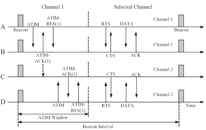
For 802.11’s PSM, nodes are assumed to be synchronized and awake at the beginning of each beacon interval. After waking up, each node stays on for a period of time known as the Ad hoc Traffic Indication Message (ATIM) window. During the ATIM window, since all nodes are guaranteed to be on, packets are advertised that have been queued since the previous beacon interval. These advertisements take the form of ATIM packets. More formally, when a node has a packet to advertise, it sends an ATIM packet to the intended destination during the ATIM window (following the rules of IEEE 802.11’s CSMA/CA mechanism). In response to receiving an ATIM packet, the destination will respond with an ATIM-ACK packet (unless the ATIM specified a broadcast or multicast destination address). When this ATIM handshake has occurred, both nodes will remain on after the ATIM window and attempt to send their advertised data packets before the next beacon interval, subject to CSMA/CA rules. If a node remains on after the ATIM window, it must keep its radio on until the next beacon interval. If a node does not receive an ATIM or ATIM-ACK (assuming unicast advertisements), it will enter sleep mode at the end of the ATIM window until the next beacon interval. This process is illustrated in Figure 2.1. The dotted arrows indicate events that cause other events to occur. NodeA sends a data packet to B, while C, not receiving any ATIM packets, returns to sleep for the rest of the beacon interval.
LISP [41] adapts 802.11 PSM to predictively wake up nodes based on overheard ATIM-ACKs. The basic idea is when data is being sent on path A → B → C, then C should remain on in any beacon interval in which it overhearsB sending an ATIM-ACK toA during the ATIM window.
of the protocol are lost. This technique is a special case of the general idea of multi-level wake-up proposed in [67]. In this paper, the authors presented the idea of generalizing power save protocols to multiple levels based on how active a node is in communicating. The basic idea is the more active a node is in communicating, the more energy it will consume to achieve a lower latency. Some scenarios are described where current power save protocols could be used with two levels as well as some future research directions. In particular, it opens many questions about interactions between the MAC and network layer, such as which routing strategy to use to minimize the number of nodes in high energy states.
2.4
Energy Consumption in the Transport Layer
The transport protocol runs over the network layer protocol. It enables end-to-end mes-sage transmission, where mesmes-sages are fragmented to chains of segments at senders and reassembled at receivers. The transport protocol usually provides the following functions: orderly transmission, flow control and congestion control, loss recovery, and possibly QoS guarantee such as timing requirement and fairness. In WSNs many new factors such as the convergent nature of upstream traffic and limited wireless bandwidth can cause con-gestion. The congestion influences normal data transmission and leads to packet loss. In addition, wireless channel introduces packet loss due to high bit-error rate, which not only affects reliability, but also wastes energy. As a result, two major problems that WSN transport protocols need to cope with are congestion and packet loss.
The traditional transport protocols that are designed for the Internet, i.e., UDP and TCP, can not be directly applied to WSNs [46]. It is well documented that UDP itself does not provide any reliability often needed for many sensor applications, nor does it offer any flow and control congestion that can lead to packet loss and unnecessary energy consumption. On the other hand, TCP suffers several drawbacks: [106]
• The overhead associated with TCP connection establishment might not justify its usage for short data collections in most event-driven applications;
• The flow and congestion control mechanism in TCP can discriminate sensor node(s) far away from the sink, and cause unfair bandwidth allocation and unfair data collections;
• It is well-known that TCP has a degraded throughput under wireless systems es-pecially with a high packet loss rate because TCP assumes all packet loss is due to congestion and triggers rate reduction whenever packet loss is detected;
• In contrast to hop-by-hop control, end-to-end congestion control in TCP has a tardy response, which needs longer time to mitigate congestion and in turn leads to more packet loss when congestion occurs;
• TCP guarantees successful transmission of each packet, which is not proper for event-driven applications.
Due to the above reasons, TCP/UDP schemes are not an appropriate transport layer solution for WSNs. In order to design an efficient transport protocol for WSNs, several factors must be taken into consideration including the topology, diversity of applications, traffic characteristics, and resource constraints. The two most significant constrains in-troduced by WSNs are the energy constrains and fairness among different geographically placed sensor nodes. The transport protocol needs to provide high energy-efficiency and flexible reliability and sometimes the traditional QoS in terms of throughout, packet loss rate and end-to-end delay.
Therefore, transport protocols for WSNs should have components including conges-tion control and loss recovery, since the two components have direct impact on energy-efficiency, reliability, and application’s QoS as explained above. There are generally two approaches to perform this task. First, design separated protocols or algorithms, respectively, for congestion control and loss recovery. Most existing protocols use this way and address either congestion control or reliable transport. With this separated and modular design, applications that need reliability can invoke only a loss recovery algorithm, or invoke a congestion control algorithm if they need to control congestion otherwise. They can so much as invoke both. For example, CODA (COngestion Detec-tion and Avoidance) [105] is a congesDetec-tion control protocol while PSFQ (Pump Slowly Fetch Quickly) [104] provides reliable transport. The joint use of them could provide full functions required by a transport protocol for WSNs. Second, design, if possible, a full-fledged transport protocol that provides congestion control and loss control in an integrated way. For example, STCP (Sensor Transmission Control Protocol) [46] imple-ments both congestion control and flexible reliability in a single protocol. For different applications, STCP offers different control policies in a way to both guarantee application requirements and improve energy efficiency.
reliability protocols can be seamlessly integrated together in an energy-efficient way. We believe there is a tradeoff between the architectural/modular design (the first approach) and integrated design with performance optimization (the second approach). The same tradeoff could also be observed between the traditional protocol stack and the cross-layer optimization in recent years.
It is an interesting topic that balancing power control in the physical layer and con-gestion control in the transport layer to enhance the overall network performance while maintaining the architectural modularity between the layers. M. Chiang [17] explored in this field by presenting a distributed power control algorithm that couples with exist-ing transmission control protocols (TCPs) to increase end-to-end throughput and energy efficiency of the network. Under the rigorous framework of nonlinearly constrained util-ity maximization, the author proved the convergence of this coupled algorithm to the global optimum of joint power control and congestion control, for both synchronized and asynchronous implementations. The rate of convergence is geometric and a desirable modularity between the transport and physical layers is maintained.
2.5
Energy Consumption in the Application Layer
The application layer in a traditional WLAN network is responsible for such things as partitioning of tasks between the fixed and mobile hosts, audio and video source encoding/decoding, and context adaptation in a mobile environment. In WSNs, we have the similar situation except that there is no load partitioning since all the nodes are mobile and peers. Although many application areas for WSNs are defined and proposed, potential application layer protocols for WSNs remain a largely unexplored region. The services offered by the application layer include: [43]
• Providing traffic management and admission control functionalities, i.e., prevent applications from establishing data flows when the network resources needed are not available;
• Performing source coding according to application requirements and hardware con-straints, by leveraging advanced multimedia encoding techniques;
• Providing primitives for applications to leverage collaborative, advanced in-network multimedia processing techniques.
Admission control has to be based on QoS requirements of the overlying application. In [43] the authors imagine that WSNs will need to provide support and differentiated service for several different classes of applications. In particular, they will need to provide differentiated service between real-time and delay-tolerant applications, and loss-tolerant and loss-intolerant applications. Moreover, some applications may require a continuous stream of multimedia data for a prolonged period of time (multimedia streaming), while some other applications may require event triggered observations obtained in a short time period (snapshot multimedia content). The main traffic classes that need to be supported are:
• Real-time, Loss-tolerant, Multimedia Streams. This class includes video and audio streams, or multi-level streams composed of video/audio and other scalar data (e.g., temperature readings), as well as meta-data associated with the stream, that need to reach a human or automated operator in real-time, i.e., within strict delay bounds, and that are however relatively loss tolerant (e.g., video streams can be within a certain level of distortion). Traffic in this class usually has high bandwidth demand.
• Delay-tolerant, Loss-tolerant, Multimedia Streams. This class includes multimedia streams that, being intended for storage or subsequent off-line processing, do not need to be delivered within strict delay bounds. However, due to the typically high bandwidth demand of multimedia streams and to limited buffers of multimedia sensors, data in this traffic class needs to be transmitted almost in real-time to avoid excessive losses.
• Real-time, Loss-intolerant, Data. This may include data from time-critical moni-toring processes such as distributed control applications. The bandwidth demand varies between low and moderate.
• Delay-tolerant, Loss-intolerant, Data. This may include data from critical moni-toring processes, with low or moderate bandwidth demand that require some form of off-line post processing.
• Delay-tolerant, Loss-tolerant, Data. This may include environmental data from scalar sensor networks, or non-time-critical snapshot multimedia content, with low or moderate bandwidth demand.
A major obstacle in these types of applications is the limited energy supply in mobile node batteries. Energy efficiency in the application layer therefore is an critical issue of research, as indicated by industry.
Let us take video transmission over wireless sensor networks as an example. Gen-erally speaking, energy in mobile devices is mainly used for computation, transmission, display, and driving speakers. Among those, computation and transmission are the two largest energy consumers. During computation, energy is used to run the operating sys-tem software, and encode and decode the audio and video signals. During transmission, energy is used to transmit and receive the radio frequency (RF) audio and video signals. In order to achieve the required signal-noise ratio (SNR), the power level of the antenna can not be too low. Therefore, computation has always been a critical concern in wire-less sensor networks. For example, energy-aware operating systems have been studied to efficiently manage energy consumption by adapting the system behavior and work-load based on the available energy, job priority, and constraints. Computational energy consumption is especially a concern for video transmission, because motion estimation and compensation, forward and inverse discrete cosine transforms (DCTs), quantization, and other components in a video encoder all require a significant number of calculations. Energy consumption in computation was recently addressed in [39], where a power rate distortion model is proposed to study the optimal trade-off between computation power, transmission rate, and video distortion.
power to provide more protection when transmitting the more important packets). This requires a “cross-layer” perspective [101] where the source and network layers are jointly considered. Specifically, the lower layers in a protocol stack, which directly control trans-mitter power, need to obtain knowledge of the importance level of each video packet from the video encoder, which is located at the application layer. On the other hand, it can also be beneficial if the source encoder is aware of the estimated channel state infor-mation (CSI) passed from the lower layers and which channel parameters at the lower layers can be controlled, so it can make smart decisions when selecting the source coding parameters to achieve the best video delivery quality. For this reason, joint consideration of video encoding and power control is a natural way to achieve the highest efficiency in energy consumption. In [54], the authors presented a general framework for the joint consideration of source coding and transmission energy consumption in a wireless video transmission system, aiming to improve the overall performance and energy efficiency. Although their work is based on WLANs and with an emphasis on system, their analysis for cross-layer implies a developing direction for sensor networks. Similar strategies have been studied in [14, 60].
QoS requirements have recently been considered as application admission criteria for sensor networks. In [76], an application admission control algorithm is proposed whose objective is to maximize the network lifetime subject to bandwidth and reliability constraints of the application. An application admission control method is proposed in [13], which determines admissions based on the added energy load and application rewards. While these approaches address application level QoS considerations, they fail to consider multiple QoS requirements (e.g., delay, reliability, and energy consumption) simultaneously, as required in WSNs.
2.6
Energy Consumption at a Cross-layer View
the bandwidth allocated to each transmitter, which naturally affects the performance of the physical layer in terms of successfully detecting the desired signals. On the other hand, as a result of transmission schedules, high packet delays and/or low bandwidth can occur, forcing the routing layer to change its route decisions. Different routing decisions alter the set of links to be scheduled, and thereby influence the performance of the MAC layer. Furthermore, congestion control and power control are also inherently coupled [17], as the capacity available on each link depends on the transmission power. Moreover, if multimedia transmissions are involved, the application layer does not require full insulation from lower layers, but needs instead to perform source coding based on information from the lower layers to maximize the multimedia performance. Existing solutions often do not provide adequate support for multimedia applications since the resource management, adaptation, and protection strategies available in the lower layers of the stack are optimized without explicitly considering the specific characteristics of multimedia applications.
The challenges brought about by WSNs call for new research on cross-layer opti-mization and cross-layer design methodologies, to leverage potential improvements of exchanging information between different layers of the protocol stack. To this aim, it is needed to specify standardized interfaces that will allow leveraging these interactions. Although a consistent amount of recent papers have focused on cross-layer design and improvement of protocols for WSNs, a systematic methodology to accurately model and leverage cross-layer interactions is still largely missing [43], and only a few work has been done for UWB-based WSNs. Most of the existing studies decompose the resource allo-cation problem at different layers, and consider alloallo-cation of the resources at each layer separately. In most cases, resource allocation problems are treated either heuristically, or without considering cross-layer interdependencies, or by considering pairwise interactions between isolated pairs of layers.
to interference-and-noise ratio above a given threshold for every link. Simulations show that considerable improvement in throughput can be obtained while also transmitting at lower power levels.
In [114], the author proposed a cross-layer design for power-efficient wireless commu-nication so that routing protocol, topology control and MAC protocol could work in an integrated manner. Location information is used through energy-efficient location ser-vice(EELS) in her power-aware design to accommodate node mobility so that efficient and stateless routing, named location-aided power-aware routing protocol (LAPAR), could be achieved. Particularly, she employed both power control (i.e., to reduce the energy by using different transmission power levels and/or coding/modulation mechanisms) and power management (i.e., to reduce the energy consumption of wireless devices by selec-tively putting them into the low-power states) to achieve maximum power saving and retain the network capacity at the same time. However, her work did not consider the spatial reuse facilitated by power control, which will increase the network capacity. Also, she did not consider the sleeping nodes, caused by power management, which will decrease the network capacity. Meanwhile, although LAPAR can provide the most power-efficient route between the source and the destination, the delay and the reliability of this path may degrade due to the increased number of hops.
J. Zhao et al [118] investigated the joint effect of MAC and PHY layers on power efficiency in IEEE 802.11a WLAN. Adopting the CSMA MAC protocol, they study the link adaptation for a power efficient transmission by selecting a proper transmission mode and power level with the aid of their derived power efficiency model. In particular, they show that the non-radio-transmission power plays an important role in the power optimization of IEEE 802.11a WLAN.
M. L. Sichitiu [89] categorized several sources of energy consumption in sensor net-works. Firstly,idle listening is the major energy consumption source for many networks. For most transceivers, the receive mode energy consumption is on the same order of magnitude as the transmission power [21, 68, 110], and most MAC protocols put the transceiver in receive mode whenever it does not transmit, whether there is the need to receive a message or not. Secondly,retransmissions resulting from collisions can be quite significant if the network load is high and the collisions frequent. Thirdly, control packet overhead (e.g., RTS, CTS, ACK) can be significant for sensor networks which, typically, have small packets. Meanwhile,unnecessarily high transmitting power not only results in higher energy consumption, but may also increase the interference at other nodes in the network. Last, sub-optimal utilization of the available resources should be considered. For example, routes that utilize the nodes with the largest (remaining) batteries should be preferred.
Considering those sources of energy consumption, as well as taking advantage of the unique characteristics of sensor networks (like stationarity and long-lived, predictable data flows), the author proposes to develop a framework for deterministic optimal energy conservation while maintaining the network real-time characteristics. In the proposed approach, sensor nodes dynamically create on-off schedules in such a way that the nodes will be awake only when needed and asleep the rest of the time. To achieve the goal, the scheme consists of two distinct phases for each flow in the network: the setup and reconfiguration phase and the steady state phase. The setup and reconfiguration phase
takes place during the initialization of the network, and subsequent to any changes in the network queries and the availability of the routes. Its goal is to set up the schedules that will be used during the steady state phase. The steady state phase takes place between consecutive setup and reconfiguration phases. It utilizes the schedule established in the setup and reconfiguration phase to forward the data to the base station. This approach does not fit cleanly in any one single layer, as it requires the collaboration of both the routing and MAC layers.
Chapter 3
Joint Effects of the Physical and
MAC Layers on Energy
Consumption of UWB-based WSNs
In this chapter, we will explore the energy consumption in UWB-based WSNs, considering the joint effect of the physical and MAC layers. At first, let us give an overview of the physical and MAC layers in UWB-based WSNs.
3.1
Network Overview
3.1.1
Physical Layer
As discussed previously, due to its resilience to multi-path [20], low transmission power and simple transceiver circuitry, UWB presents itself as a good candidate for the Physical Layer (PHY) of wireless multi-hop networks, both for high and low data rate applications [82].
UWB radio communications are an extreme form of spread spectrum communications. The FCC has defined a UWB device as any device with a -10dB fractional bandwidth, FBW, greater than 0.20 or occupying at least 500MHz of the spectrum [19]:
FBW = 2
fH −fL
fH +fL
wherefH is the upper frequency of the -10dB emission point, andfLis the lower frequency
of the -10dB emission point. The FCC also regulated the spectral shape and maximum power spectral density (≈-41dBm/MHz) of the UWB radiation in order to limit the interference with other communication systems.
The UWB signals generation methods can be grouped in two major categories:
• Single-Band (SB) based: employing one single transmission frequency band, and
• Multi-Band (MB) based, employing two or more frequency bands, each with at least 500MHz bandwidth.
In the SB solution, the UWB signal is generated using very short, low duty-cycle, base-band electrical pulses with appropriate shape and duration. Due to the carrier-less char-acteristics (no sinusoidal carrier to raise the signal to a certain frequency band) these UWB systems are also referred to as carrier-free or Impulse Radio (IR)-UWB communi-cation systems [109]. The MB UWB systems can be implemented carrier less (different pulse shapes/lengths are used according to the frequency band) or carrier based (multi-carrier like) [6, 48, 97, 108].
Two competing UWB standards have been proposed by IEEE 802.15.3a Task Group (TG3a), i.e., Multi-Band Orthogonal Frequency Division Multiplexing (MB-OFDM) UWB [7–9, 44], and Direct Sequence (DS) UWB [34, 35]. Due to their significant dif-ference, IEEE announced in January 2006 that it had given up trying to formulate a uniform UWB standard and had left it to the producers to make their own standards. In 2007, DS-UWB was added into IEEE 802.15.4a as a standard, while MB-OFDM UWB was adopted by the WiMedia Alliance which published ECMA-368 in 2008. In this work, we will analyze and compare the energy consumption of the two UWB technologies, com-bining with the effects of the protocols in other layers.
has several nice properties, including the ability to efficiently capture multi-path energy with a single RF chain, insensitivity to group delay variations, and the ability to deal with narrowband interferers at the receiver without having to sacrifice either sub-bands or data rate.
Figure 3.1 illustrates how the OFDM symbols are transmitted in a MB-OFDM system. In this example, it has been implicitly assumed that the time-frequency coding (TFC) is performed across just three OFDM symbols. In a MB-OFDM system, a guard interval (9.5 nanoseconds) is appended to each OFDM symbol and a zero-padded prefix (60.6 nanoseconds) is inserted at the beginning of each OFDM symbol. The guard interval ensures that there is sufficient time for the transmitter and receiver to switch to the next carrier frequency. A zero-padded prefix provides both robustness against multi-path and eliminates the need for power back-off at the transmitter.
Figure 3.1: Example of TF coding for an MB-OFDM system.
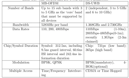
The system parameters for the 110 Mb/s, 200 Mb/s, and 480 Mb/s modes of MB-OFDM solution are given in Table 3.1.
proposals sent to the IEEE 802.15.3a standardization committee by the proponents of this technology, the DS-UWB technique is scalable and can achieve data rates in excess of 1 Gbps. The technical reason behind using DS-UWB is the propagation benefits of ultra-wide band pulses, which experience no Rayleigh fading.
The system parameters for the DS-UWB solution are also given in Table 3.1.
3.1.2
MAC Layer
Because of their low end-to-end throughput and poor scalability in a wireless multi-hop network, single-channel random access protocols such as CSMA/CA are not an efficient solution. To further improve network performance and also increase network capacity for wireless multi-hop networks, a favorable solution is to enable a network node to work on multiple channels instead of only on a single fixed channel, because multiple transmissions can take place without interfering. When cost and compatibility are the concern, one transceiver on a radio is a preferred hardware platform. Since only one transceiver is available, only one channel is active at a time in each network node. However, different
Table 3.1: MB-OFDM and DS-UWB System Parameters.
MB-OFDM DS-UWB
Number of Bands Up to 15 sub bands with 3 to 5 GHz as the ‘core’ band that must be supported by all devices
2 (independent, 3 to 5 GHz and 6 to 10 GHz)
Bandwidth 528MHz per band 1.368GHz and 2.736GHz Data Rates 110, 200, 480Mbps 110Mbps (1-10m);
200Mbps-480Mbps(0-1m); recently 1.3Gbps (2-3m claimed)
Chip/Symbol Duration Symbol: 312.5ns, including 9.5ns guard interval, 60.6ns ISI interval and 242.4ns in-formation duration
Chip: 731ps (low band); 365ps (high band)
Modulation BPSK, QPSK BPSK(mandatory),
4-BOK(optional) Multiple Access Time/Frequency
Interleav-ing
nodes may operate on different channels simultaneously. To coordinate transmissions between network nodes under this situation, many multi-channel MAC protocols have been proposed for multi-hop wireless networks [37, 42, 47, 92, 111, 112].
Dual Busy Tone Multiple Access [37] divides a common channel into two sub-channels, one data channel and one control channel. Busy tones are transmitted on a separate control channel to avoid hidden terminals, while data is transmitted on the data channel. This scheme uses only one data channel and is not intended for increasing throughput using multiple channels.
Wu et al. [111, 112] propose a protocol that assigns channels dynamically, in an on-demand style. In this protocol, called Dynamic Channel Assignment (DCA), they main-tain one dedicated channel for control messages and other channels for data. Each host has two transceivers, so that it can listen on the control channel and the data channel si-multaneously. RTS/CTS packets are exchanged on the control channel, and data packets are transmitted on the data channel. In RTS packet, the sender includes a list of pre-ferred channels. On receiving the RTS, the receiver decides on a channel and includes the channel information in the CTS packet. Then, DATA and ACK packets are exchanged on the agreed data channel. Since one of the two transceivers is always listening on the control channel, multi-channel hidden terminal problem does not occur. This protocol does not need synchronization and can utilize multiple channels with little control mes-sage overhead. But it does not perform well in an environment where all channels have the same bandwidth. When the number of channels is small, one channel dedicated for control messages can be costly. In case of IEEE 802.11b, only 3 channels are available, so having one control channel results in 33% of the total bandwidth as the control overhead. On the other hand, if the number of channels is large, the control channel can become a bottleneck and prevent data channels from being fully utilized.
Jain et al. [47] propose a protocol that uses a scheme similar to [111] that has one control channel and N data channels, but selects the best channel according to the chan-nel condition at the receiver side. The protocol achieves throughput improvements by intelligently selecting the data channel, but still has the same disadvantages as DCA.
Compared to the above works, the Multi-channel MAC (MMAC) protocol proposed by So and Vaidya [92] operates with one transceiver per host. Also, it does not require a dedicated control channel. Instead, it requires clock synchronization among all the hosts. At the start of each interval, there is an Ad hoc Traffic Indication Messages (ATIM) window, during which all hosts are required to listen to a default common channel in order to exchange traffic indication messages. During this ATIM window hosts do not exchange data packets. So this duration of time is an overhead in this scheme. However, the authors demonstrated that it achieves better throughput than maintaining a separate control channel.
Figure 3.2: Process of Channel Negotiation and Data Exchange in MMAC.
3.2
Energy Consumption Model of the Physical and
MAC layers
Given the overview of the physical and MAC layers in UWB WSNs, next we will propose our energy consumption model to study the joint effect of the physical and MAC layers. To be specific, we assume that MMAC is adopted as the MAC protocol, and for physical layer, the UWB technology is applied.
3.2.1
Energy Consumption Components
As mentioned by [28], significant power may be consumed not only by the radio transmis-sion, but also by many other sources: operation of the transceiver, computation, channel sensing and etc. This denotes that even in the idle slot, the node consumes some power. To investigate the overhead of these components on the energy consumption, we model them as two parts at certain states: the base power sink, and the incremental part power sink; while the states include idle state, transmitting state and receiving state. Suppose the base power isPbase which is the power required for basic operation. This includes the
power consumed by the circuits, the power amplifier and etc. The incremental part due to transmitting, receiving and channel sensing (idle) is given by Ptrans, Precv and Pidle.
Then the total power in each state, PT X,PRX and PI, are respectively given by
PT X = Pbase+Ptrans (3.2)
PRX = Pbase+Precv (3.3)
PI = Pbase+Pidle (3.4)
Different values of Pbase place different weight on the overhead of energy consumption.
For simplicity, Pbase is normalized to 1.
3.2.2
State Duration and Energy Consumption
For ad hoc networks, the actual transmission duration of a frame depends on the frame size and the PHY (UWB) mode used. The transmission duration of a frame with size L in MB-OFDM UWB mode is given by:
TdataM B(L) =TpreM B+TheadM B +TsymM B×NsymM B(L) (3.5)
where NM B
sym(L) is the number of OFDM symbols needed to transmit L data bits and is
given by:
NsymM B(L) =⌈ L
TM B
inf ×RM B
⌉ (3.6)
Here function⌈x⌉returns the smallest integer value greater than or equal tox. The other notations are listed in Table 3.2.
If the frame is transmitted in DS-UWB mode, its transmission duration is given by:
TdataDS(L) =TpreDS+TheadDS +TchipDS ×NchipDS(L) (3.7)
Table 3.2: Timing Related Parameters for MB-OFDM. Parameters Values
TM B
sym: Symbol length 312.5ns
TM B
inf : Information duration 242.4ns
TM B
pre : PLCP Preamble 9.375us
TM B
head: PLCP Header 3.75us
RM B: Data rate 110Mbps
Table 3.3: Timing Related Parameters for DS-UWB.
Parameters Values
TDS
pre: Preamble duration Nominal preamble: 15µs
(by default) TDS
head: PHY header, MAC
header, and header check sequence(HCS)
PHY header=24 bits, MAC header=80 bits, HCS=16 bits
TDS
chip: Chip duration 731ps (low band); 365ps
where NchipDS(L) is the number of DS-UWB chips needed to transmit L data bits. By default, BPSK is used to modulate data in which each symbol carries only a single data bit. Considering we have 24 chips per symbol [29], NDS
chip(L) is given by:
NchipDS(L) = 24×L (3.8)
Other notations are listed in Table 3.3.
The data transmission in MMAC is completed by a sequence of packet exchanges. In a sequence of packet exchange, a node may be in different states. First, the sender will negotiate with the receiver on which channel to use, during the ATIM window, through exchanging ATIM, ATIM-ACK, and ATIM-RES packets. After selecting the channel, the sender can transmit data to the receiver, as shown in Figure 3.3. If the source-destination pairs that are closely placed happen to choose the same channel, the senders and receivers will exchange RTS/CTS packets and transmit data as the original IEEE 802.11 DCF, as shown in Figure 3.4. Then, the sender changes to idle state at the end of transmission for a time interval ofTsif s. After that, it may receive ACK frame, or still in idle time for
Tacktimeout, which depends on whether the data transmission succeeds or not.
A
B
DAT A
ACK DIF S
SIF S
Figure 3.3: Data Transmission Sequence.
For a tagged node, it may encounter five types of events in each time slot and the energy consumption for each event is:
(1) The tagged node transmits to one of its neighbors and succeeds. Note there are two possibilities. If the RTS-CTS exchange is not involved,
Esuc1 = PT X ×(T(Ldata) +T(Latim) +T(Latim−res)) +PI ×(Tsif s+Tdif s) +
If the RTS-CTS exchange is involved,
Esuc2 = PT X×(T(Ldata) +T(Lrts) +T(Latim) +T(Latim−res)) +
+PI ×(3×Tsif s+Tdif s) +
+PRX ×(T(Lcts) +T(Lack) +T(Latim−ack)). (3.10)
(2) The tagged node transmits to one of its neighbors but fails due to failure of data packet transmission. Similarly, there are also two possibilities. If the RTS-CTS exchange is not involved,
Ef ail1 = PT X ×(T(Ldata) +T(Latim) +T(Latim−res)) +
+PI ×(Tsif s+Tacktimeout) +PRX ×T(Latim−ack). (3.11)
If the RTS-CTS exchange is involved,
Ef ail2 = PT X×(T(Ldata) +T(Lrts) +T(Latim) +T(Latim−res)) +
+PI ×(3×Tsif s+Tacktimeout) +
+PRX×(T(Lcts) +T(Latim−ack)). (3.12)
(3) The tagged node does not transmit, while one of its neighbors transmits to it and
succeeds. If the RTS-CTS exchange is not involved,
Eother,suc1 = PRX×(T(Ldata) +T(Latim) +T(Latim−res)) +PI ×(Tsif s+Tdif s) +
+PT X×(T(Lack) +T(Latim−ack)). (3.13)
If the RTS-CTS exchange is involved,
Eother,suc2 = PRX ×(T(Ldata) +T(Lrts) +T(Latim) +T(Latim−res)) +
+PI ×(3×Tsif s+Tdif s) +
+PT X×(T(Lcts) +T(Lack) +T(Latim−ack)). (3.14)
(4) The tagged node does not transmit, while one of its neighbors transmits to it but fails due to failure of data packet transmission. If the RTS-CTS exchange is not involved,
Eother,f ail1 = PRX ×(T(Ldata) +T(Latim) +T(Latim−res)) +
+PI ×(Tsif s+Tacktimeout) +PT X×T(Latim−ack). (3.15)
If the RTS-CTS exchange is involved,
Eother,f ail2 = PRX ×(T(Ldata) +T(Lrts) +T(Latim) +T(Latim−res)) +
+PI ×(3×Tsif s+Tacktimeout) +
+PT X×(T(Lcts) +T(Latim−ack)). (3.16)
(5) The tagged node neither transmits nor receives, therefore it keeps sleeping during the slot:
Eidle = PI ×Tslot. (3.17)
3.2.3
Transmission Probability
In order to derive the probabilities for each event defined above, we need to use an important variable: transmission probability τ that the node transmits a packet in a generic slot time. Intuitively, τ depends on the collisions a node may encounter. In MMAC, the collision occurs under two circumstances. The first is when multiple nodes start sending ATIM packets at the beginning of a slot. To avoid such collisions, we let each node wait for a random back-off time before sending an ATIM packet. The back-off time is chosen in the range [0, ω], where ω is called contention window. At the first transmission attempt, ω is set equal to the minimum value CWmin. The back-off time
counter is decremented at the beginning of each slot. When the back-off time reaches zero, the node transmits. If another collision occurs, the contention window is doubled, up to a maximum valueCWmax = 2mCWmin, where m is defined as the maximum
back-off stage. On the other hand, if the transmission is successful, the node will divide its contention window size by 2. Recall the Binary Exponential Back-off (BEB) used in IEEE 802.11 DCF, if the transmission is successful, the node will reset its contention window to the minimum. However, this mechanism causes a very large variation of the contention window size, and degrades the performance of a network when it is heavily loaded since each new packet starts with the minimum contention window, which can be too small for the heavy network load. Compared with BEB, our back-off scheme is more efficient. The comparison result by simulation will be shown in the next section.
The other circumstance under which the collision occurs in MMAC is when two source-destination pairs that are closely placed choose the same channel. Then they have to contend just as they contend for sending the ATIM packet. In this case, we use the same back-off scheme as we proposed in the first case. Based on the analytical evaluation of the saturation throughput proposed in [10], we construct a Markov chain model for the back-off window size. Based on this model, we can derive the transmission probabilityτ. We assume each node has immediately a packet available for transmission, after the completion of each successful transmission. Letb(t) be the stochastic process representing the back-off time counter for a given node at timet. DefineW =CWmin for convenience.
Denote Wi = 2iW, where i ∈ [0, m] is called back-off stage. Let s(t) be the stochastic
process representing the back-off stage of the node at timet.
· · · · · · · · · · · · · · · · · · · · · · · · · · · · · · · · · · · · · · · · · · · · · · · · 1 1 1 1 1 1 1 1 1 1 1 1 1 1 1 1 1 1 1 1 1 1 1 1 1 1 1 1 1 1
0,0 0,1 0,2 0, W0−2 0, W0−1
(1−p)/W0
(1−p)/W0
(1−p)/W0
(1−p)/W0
(1−p)/W0
(1−p)/W0
1,0 1,1 1,2 1, W1−2 1, W1−1
p/W1
p/W1
p/W1
i−1,0 i−1,1 i−1,2 Wii−−1−1,2 Wi−1,
i−1−1
p/Wi
p/Wi
p/Wi (1−p)/Wi−1
(1−p)/Wi−1
i,0 i,1 i,2 i, Wi−2 i, Wi−1
p/Wi+1
p/Wi+1
p/Wi+1
i+ 1,0 i+ 1,1 i+ 1,2 Wi+ 1, i+ 1,
i+1−2 Wi+1−1
(1−p)/Wi
(1−p)/Wi
p/Wm
p/Wm p/W
m
p/Wm
m,0 m,1 m,2 m, Wm−2 m, Wm−1
referred to as retransmission probability. Based on the above assumptions, we model the bi-dimensional process{s(t), b(t)}with the discrete-time Markov chain shown in Fig-ure 3.5. From the Markov chain, we have the following non null one-step transition probabilities:
P{i, k|i, k+ 1} = 1, k ∈[0, Wi−2], i∈[0, m],
P{i, k|i+ 1,0}= (1−p)/Wi, k∈[0, Wi−1], i∈[0, m−1],
P{i, k|i−1,0}=p/Wi, k ∈[0, Wi−1], i∈[1, m],
P{0, k|0,0}= (1−p)/W0, k ∈[0, W0−1],
P{m, k|m,0}=p/Wm, k ∈[0, Wm−1],
(3.18)
where the following short notation is adopted:
P{i1, k1|i0, k0}=P{s(t+ 1) =i1, b(t+ 1) =k1|s(t) =i0, b(t) =k0}.
The first equation in (3.18) is derived from our assumption that, at the beginning of each time slot, the back-off time is decreased by 1. The second equation means when a successful transmission occurs at back-off stagei+1, the back-off stage decreases, and the new back-off is initially uniformly chosen in the range [0, Wi−1]. The third equation of
(3.18) means when an unsuccessful transmission occurs at back-off stage i−1, the back-off stage increases, and the new initial back-back-off value is uniformly chosen in the range [0, Wi−1]. The fourth equation models the fact that once the back-off stage reaches the
minimum value 0, it is not decreased any more. Finally, the fifth equation means once the back-off stage reaches the maximum valuem, it is not increased in subsequent packet transmissions.
Let bi,k = limt→∞P{s(t) = i, b(t) = k}, i ∈ [0, m], k ∈ [0, Wi−1] be the stationary
distribution of the chain. Then we have
b0,0·(1−p) +b1,0·(1−p) =b0,0,
bi−1,0·p+bi+1,0·(1−p) =bi,0, 0< i < m,
bm−1,0·p+bm,0·p=bm,0.
(3.19)
Combing the equations in (3.19), we obtain the following relationship:
bi,0 =b0,0·
pi
For each k ∈[1, Wi−1], we have
b0,k = WW0−0k(1−p)(b0,0+b1,0),
bi,k= WWi−ik(p·bi−1,0+ (1−p)bi+1,0), 0< i < m,
bm,k = WWmm−k ·p·(bm−1,0+bm,0).
(3.21)
With the relations (3.20), we can rewrite the equations in (3.21) as
bi,k =
Wi−k
Wi
bi,0, i∈[0, m], k ∈[0, Wi−1]. (3.22)
Making use of the relations (3.20) and (3.22), all the valuesbi,k are expressed as functions
of the values b0,0 and of the retransmission probability p. b0,0 can finally be derived by
applying the normalization condition:
1 =
m
X
i=0
Wi−1
X k=0 bi,k = m X i=0
bi,0
Wi−1
X
k=0
Wi−k
Wi
=
m
X
i=0
bi,0
Wi+ 1
2
= b0,0 2
h W
m−1
X
i=0
(2p)i+ (2p)m
1−p
+ 1 1−p
i
, (3.23)
thus,
b0,0 =
2(1−2p)(1−p)
(1−2p)(W + 1) +pW(1−(2p)m). (3.24)
of the back-off stage, it can be expressed as
τ =
m
X
i=0
bi,0
= b0,0·
m
X
i=0
pi
(1−p)i
= b0,0·
(1−p)m+1−pm+1
(1−2p)(1−p)m
= 2[(1−p)
m+1−pm+1]
[(1−2p)(W + 1) +pW(1−(2p)m)](1−p)m−1. (3.25)
Therefore, τ is dependent on the retransmission probability p. For the case of sending ATIM packets, if we ignore any channel error, pis equal to the probability that in a time slot at least one of the N neighboring nodes transmit(s) ATIM packet(s), thus we have
patim = 1−(1−τatim)N, (3.26)
where patim is the retransmission probability of the ATIM packet, andτatim is the
trans-mission probability of the ATIM packet. Obviously, the relationship between patim and
τatim is coincident with Equation (3.25). Equations (3.25) and (3.26) represent a
non-linear system in the two unknown variables τatim and patim, which can be solved using
numerical techniques.
For the case of sending RTS packets, the retransmission probability of the RTS packet is determined by the successful transmission probability of RTS, CTS, data, and ACK packets, i.e.,
prts = 1−ps(seq), (3.27)
whereps(seq) =ps(Lrts)ps(Lcts)ps(Ldata)ps(Lack). Notice the fact that the length of ACK
and CTS frames is much shorter than RTS and data frames, the successful transmission probabilities of ACK and CTS can be approximated to be 1. Therefore, in order to calculate prts, we need to calculate ps(Lrts) and ps(Ldata) first.