Efficient Decomposition Techniques for Traffic Grooming Problems in Optical Networks.

(1)

ABSTRACT

WANG, HUI. Efficient Decomposition Techniques for Traffic Grooming Problems in Optical Networks. (Under the direction of Dr. George N. Rouskas.)

Traffic grooming refers to a class of optimization problems developed to address the gap between the wavelength capacity and the traffic demands of individual connections in optical WDM networks. In this work, we focus on static traffic grooming problem and its subproblems, with an objective function of minimizing the total number of lightpaths. A lightpath is a path of physical links with a particular wavelength reserved on each link, and it is used as a metric of network cost.

We first review the existing work in this area and a typical integer linear program (ILP) formulation in the literature, and we identify two challenges related to this formulation in terms of scalability and wavelengths fragmentation. We then make three contributions that address the scalability challenges.

First, we propose a new solution approach that decomposes the traffic grooming problem into two subproblems that are solved sequentially: (1) the virtual topology and traffic routing (VTTR) subproblem, that does not take into account physical topology constraints, and (2) the routing and wavelength assignment (RWA) subproblem, that reconciles the virtual topology determined byVTTRwith the physical topology. The decomposition is exact when the network is not wavelength limited. We also propose three algorithms that use a partial LP relaxation technique driven by lightpath utilization information to solve theVTTRsubproblem efficiently. Our approach delivers a desirable tradeoff between running time and quality of the final solution. Second, instead of viewing the network as a flat entity, we further consider networks with hierarchies, where the second level of hierarchy consists of hub nodes, and the first level is formed by the remaining nodes. Hierarchical traffic grooming facilitates the control and management of multigranular WDM networks. We first survey heuristic hierarchical grooming algorithms. We then apply the above decomposition approach onto hierarchical traffic grooming. We define the hierarchical virtual topology and traffic routing (H-VTTR) problem, and we present a suite of ILP formulations to solve it. The formulations represent various tradeoffs between solution quality and running time. We also explore the performance of the formulations under various direct lightpath thresholds, traffic loads, and number of hubs. The formulations are cross-compared with the baseline VTTR formulation.

(2)

(3)

c

(4)

Efficient Decomposition Techniques for Traffic Grooming Problems

in Optical Networks

by Hui Wang

A dissertation submitted to the Graduate Faculty of North Carolina State University

in partial fulfillment of the requirements for the Degree of

Doctor of Philosophy

Operations Research Computer Science

Raleigh, North Carolina

2013

APPROVED BY:

Dr. Rudra Dutta

Co-chair of Advisory Committee

Dr. Yahya Fathi

(5)

DEDICATION

To my parents,

(6)

BIOGRAPHY

Hui Wang is a Ph.D. candidate in Opertions Research with co-major in Computer Science at North Carolina State University (NCSU). She was born in Shijiazhuang, Hebel, China in 1985, and spent the first 18 years of life in her hometown. She received her B.S. degree in Applied Mathematics from Peking University in July 2007. She directly joined the Ph.D. program in Operations Research at NCSU after graduating from college. She received her Master degrees in Operations Research and Statistics from NCSU in 2009 and 2011, respectively.

She has successfully completed the Graduate Leadership Development Series program in Spring, 2013. She received a 2013 SAS Summer Fellowship in Revenue Management and Pricing Optimization, and was recognized as a SAS Student Ambassador in 2011. She is a member of the Honor Societies Mu Sigma Rho, Omega Rho, and Phi Kappa Phi. She has interned at United Airlines Inc., for two summers in 2010 and 2011. During her graduate study, she has been actively involved in student organizations. She is the secretary of NCSU Women in Computer Science. She served as the President of the Operations Research Graduate Student Association and the NCSU INFORMS Student Chapter, and the Chair of the University Graduate Student Association Teaching Effectiveness Committee in the academic year of 2009. She is also a student member of the Institute of Electrical and Electronics Engineers (IEEE) and the Institute for Operations Research and the Management Sciences (INFORMS)

(7)

ACKNOWLEDGEMENTS

I would like to thank my advisor, Dr. George N. Rouskas, for his dedicated guidance and mentorship, especially in multi-disciplinary study and research. Without your help, this thesis would not be possible. I am grateful for your encouragement in my exploring many oppor-tunities. You have definitely set my direction and attitude in professional career. I am also very grateful to the rest of my committee: Dr. Rudra Dutta, for his valueable suggestions; Dr. Yahya Fathi and Dr. William Stewart, for their insightful comments and questions.

Much gratitude to my parents, Ping Zhang and Haoxu Wang, who raised me, provided me the best education opportunities, and gave me constant love and support. Thank you for believing in me.

To Shengfan Zhang, Andrea Villanes, Queqing Wang, Yuan Geng, Ziyu Xiao, Min Li, Yao Liu and all of my friends, thank you for bringing so much fun into my graduate study, and thank you for sharing my happy and sad moments. Special thanks to Baris Kacar, you made me want to be a better person.

(8)

TABLE OF CONTENTS

LIST OF TABLES . . . vii

LIST OF FIGURES . . . .viii

Chapter 1 Traffic Grooming, ILP Formulation, and Challenges . . . 1

1.1 Introduction and Related Work . . . 1

1.2 The Concept of Traffic Grooming . . . 3

1.3 Basic ILP Formulation and Challenges . . . 5

1.4 Traffic Grooming Subproblems by Logical Decomposition . . . 8

1.5 Challenges . . . 10

1.5.1 Scalability . . . 10

1.5.2 Wavelength Fragmentation . . . 11

1.6 Thesis Contributions and Organization . . . 13

Chapter 2 A Novel Decomposition Approach and Efficient Algorithms . . . 15

2.1 A New Decomposition of Traffic Grooming . . . 15

2.1.1 Virtual Topology and Traffic Routing (VTTR) . . . 15

2.1.2 Routing and Wavelength Assignment (RWA) . . . 17

2.1.3 Sequential Solution to the VTTR and RWA Problems . . . 17

2.2 Three Efficient Algorithms for VTTR . . . 18

2.2.1 Partial LP Relaxation ofVTTR . . . 19

2.2.2 Lightpath Utilization . . . 21

2.2.3 VTTR-rlx(Uthr) . . . 21

2.2.4 VTTR-rlx(Ul, Uh) . . . 22

2.2.5 VTTR-rlx(Ul, Uh)-Int . . . 24

2.3 Numerical Results . . . 24

2.3.1 VTTR-rlx(Uthr) . . . 25

2.3.2 VTTR-rlx(Ul, Uh) . . . 27

2.3.3 VTTR-rlx(Ul, Uh)-Int . . . 32

2.3.4 Wavelength Fragmentation . . . 33

Chapter 3 Hierarchical Virtual Topology and Traffic Routing . . . 36

3.1 Related Work in Hierarchical Grooming . . . 37

3.1.1 Ring Networks . . . 37

3.1.2 Torus, Tree, and Star Networks . . . 39

3.1.3 General Topology Networks . . . 40

3.1.4 Discussion . . . 44

3.2 Hierarchical VTTR Problem and Variants . . . 45

3.2.1 H-VTTR with Clustering (HC-VTTR) . . . 49

3.2.2 Hierarchical Grooming with Direct Lightpaths . . . 49

(9)

3.3.2 Quality of Solution and Scalability . . . 53

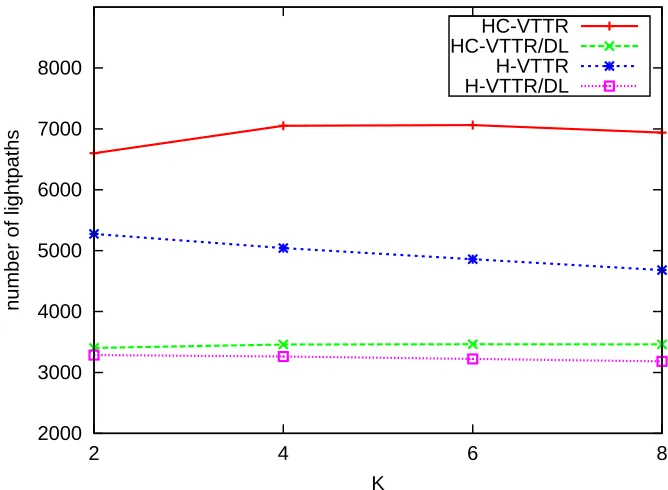
3.3.3 Effect of Number of Hubs . . . 56

Chapter 4 Multi-class Traffic Grooming. . . 60

4.1 Introduction . . . 60

4.2 Multi-Class Traffic Grooming . . . 60

4.3 Multi-Class Virtual Topology and Traffic Routing (MC-VTTR) . . . 61

4.4 Multi-Class Grooming Algorithms . . . 63

4.4.1 Separate Formulation . . . 63

4.4.2 Baseline Formulation . . . 63

4.5.1 Quality of Solution . . . 64

4.5.2 CPU Time . . . 65

Chapter 5 Conclusions and Future Work . . . 76

5.1 Future Work . . . 77

References. . . 79

Appendix . . . 83

(10)

LIST OF TABLES

(11)

LIST OF FIGURES

Figure 1.1 Illustration of an optical WDM network and traffic grooming . . . 5

Figure 1.2 Illustration of virtual topology design and traffic routing subproblem . . 9

Figure 1.3 Illustration of lightpath routing subproblem . . . 9

Figure 1.4 Illustration of wavelength assignment subproblem . . . 10

Figure 1.5 CPLEX running time to find an optimal solution, as a function ofN the number of nodes of the ring network . . . 11

Figure 1.6 Wavelength usage comparison for five traffic instances, ring network with N = 6 nodes . . . 12

Figure 2.1 CPU time, as a function ofH,N = 12, iterative algorithmVTTR-rlx(Uthr) 26 Figure 2.2 Quality of solution as a function ofH, algorithmVTTR-rlx(Uthr),tmax = 30 . . . 27

Figure 2.3 CPU time as a function ofN, iterative algorithm VTTR-rlx(Uthr),H = 0.8, tmax= 30 . . . 28

Figure 2.4 Solution quality as a function of (Ul, Uh),tmax= 30 . . . 29

Figure 2.5 CPU time as a function of (Ul, Uh),N = 16 . . . 30

Figure 2.6 CPU time as a function ofUl,N = 24, tmax=30 . . . 31

Figure 2.7 CPU time as a function ofN, (Ul, Uh) = (0.5,0.6), tmax = 30 . . . 32

Figure 2.8 CPU time comparison as a function of network sizeN,tmax= 30 . . . . 33

Figure 2.9 Solution Quality for VTTR-rlx(Ul, Uh)-Int, N=8, 16, 24, tmax=30 . . . . 34

Figure 2.10 Running time (sec) forVTTR-rlx(Ul, Uh)-Int, N=8, 16, 24, tmax=30 . . 34

Figure 2.11 Wavelength usage comparison, 6-node ring network,tmax= 12 . . . 35

Figure 3.1 Hierarchical ring architecture with 12 access and 4 backbone nodes . . . 38

Figure 3.2 Ring architecture with 4 super-nodes, each of size 4 . . . 39

Figure 3.3 A 32-node network, partitioned into eight first-level clustersB1,· · · , B8, with the corresponding hubs at the second level of the hierarchy . . . 41

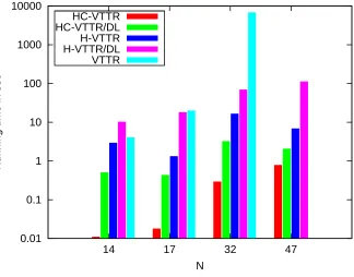
Figure 3.4 14-node NSFnet . . . 52

Figure 3.5 17-node German Network . . . 53

Figure 3.6 47-node Network from [1] . . . 54

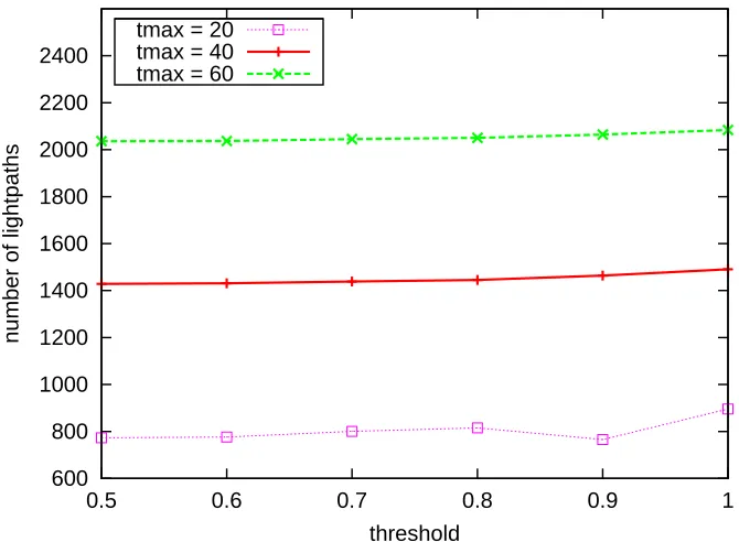
Figure 3.7 Objective value of H-VTTR/DL as a function of threshold value θ . . . . 55

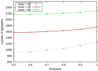
Figure 3.8 Objective value of HC-VTTR/DL as a function of threshold valueθ . . . 56

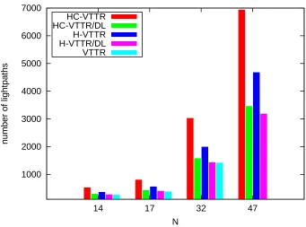
Figure 3.9 Objective value comparison,tmax = 40 . . . 57

Figure 3.10 CPU time comparison,tmax= 40 . . . 58

Figure 3.11 Objective value comparison, 32-node network,K= 8 hubs . . . 58

Figure 3.12 Objective value comparison, 47-node network,tmax = 40 . . . 59

Figure 3.13 CPU time comparison, 47-node network,tmax= 40 . . . 59

Figure 4.1 Number of lightpaths, 14-node network,K = 3 traffic classes . . . 66

Figure 4.2 CPU time of 14-node network, K= 3 traffic classes . . . 66

Figure 4.3 Number of lightpaths of 14-node network, K= 4 traffic classes . . . 67

(12)

Figure 4.10 CPU time of 17-node network,K= 4 traffic classes . . . 70

Figure 4.11 Number of lightpaths of 17-node network,K= 5 traffic classes . . . 71

(13)

Chapter 1

Traffic Grooming, ILP Formulation,

and Challenges

1.1 Introduction and Related Work

In the modern world, communication services delivered via the Internet touch all of society and affect all aspects of human life. To accommodate the exponential growth of demand in communications, infrastructure that can support ever increasing amounts of traffic is highly needed. Optical networks have been commonly used as the backbone infrastructure of Internet services, since they deliver high performance in terms of both throughput and QoS. The physical structure of an optical network consists of a set of nodes and optical fibers that interconnect them. With the help of wavelength division multiplexing (WDM) technology, it is possible to transmit traffic on different wavelengths within the same optical fiber simultaneously. The data rate of a single wavelength can be up to 40 Gbps, while higher rates are becoming commercially available. Therefore, the capacity of each wavelength can be significantly higher than the magnitude of individual traffic demands.

The concept of traffic grooming was introduced in the mid-1990s to address the gap between the channel capacity and individual traffic demands in optical networks. The key idea is to aggregate individual traffic requests onto wavelengths so as to improve bandwidth utilization across the network and minimize the use of network resources. Many variants of traffic grooming have been studied in the literature. Online versions of the problem target network environments in which traffic demands arrive in real time. Since future demands are not known in advance, the main objective of online problems is to minimize blocking probability or maximize throughput. Heuristics for solving online traffic grooming problems have been proposed in [16, 21, 22, 44].

(14)

(ILPs) and assume the existence of a traffic matrix representing the demands between node pairs. Basic ILP formulations of the problem are available in [14] and [46]. Typically, the objective is to minimize the total network cost while satisfying all demands (e.g., as in [10, 25]), or to maximize the total revenue by satisfying as many traffic demands as possible given certain capacity (wavelength) constraints (e.g., as in [46]). Since electronic equipments that terminate lightpaths represent a large fraction of the overall network cost, the number of lightpaths established to carry the traffic demands is usually taken as the metric to minimize [25]. Other cost functions have also been considered, including the electronic switching cost of grooming traffic between lightpaths at intermediate switches [13], and power consumption in optical networks [43].

One essential concern about the ILP formulations is that they are solvable only for small network topologies [43]. For larger topologies representative of deployed networks, the ILP formulation cannot be solved to optimality within reasonable amounts of time (e.g., a few hours). Therefore, the offline problem has been addressed either using heuristic algorithms [8,45] or by manipulating the ILP formulation using decomposition or column generation techniques. In [21], the original ILP is decomposed into two simpler ILPs: one that addresses only the traffic routing and lightpath routing subproblems and is solved first; and another that addresses the wavelength assignment problem only and takes as input the solution of the first ILP. In [41], a level decomposition method is introduced to address the layered routing and multi-rate connection characteristics of traffic grooming. In [29], the objective is to design a ring network that is able to satisfy any request graph with maximum degree at mostδ. The cases of δ= 2 and δ= 3 were solved by graph decomposition.

Column generation techniques were developed in [12, 37]. Given that the main difficulty in solving the problem has to do with selecting from among an exponential number of possible paths to route the traffic demands, a heuristic algorithm using column generation for a path-based formulation of the problem was developed in [12]. The key idea was to generate an optimal subset of paths efficiently. A hierarchical optimization method was proposed in [37]. The method first deals with the grooming and routing decisions using column generation to find the dual bounds and a rounding heuristic to find an integral solution; wavelength assignment was then carried out in a second step.

(15)

traffic grooming problem for mesh networks. In many-to-one mode, several source nodes com-municate with one single destination node, like in resource discovery and data collection. [36] addresses the many-to-one traffic grooming problem such that all traffic requests are satis-fied with the least number of required hight layer light termination equipments, and together minimizing the total number of used wavelengths, with a dynamic programming style heuris-tic algorithm. Many-to-many communication allows several users interact with each other. For example, distance learning, multimedia conference, and distributed computing all require many-to-many communication mode. In many-to-many communication mode, also called group communication mode, a session is formed by members (which refer to a group of users), where each member in this group transmits its traffic to every other member in the same group, [33]. Usually, the requirements for bandwidth for these user applications are much lower than the capacity of single wavelength. Thus, it becomes substantial to groom users’ traffic demands at optical level. Many-to-many communication requires that each node in WDM network is capable of duplicating the incoming traffic into several copies, each copy going to a different output port.

Existing approaches to obtaining optimal solutions to the traffic grooming problem face serious scalability challenges as well as wavelength fragmentation issues; we discuss each chal-lenge in Sections 1.5.1 and 1.5.2, respectively. The lack of scalability of optimal methods makes it difficult to characterize the performance of heuristic algorithms in realistic topologies, and severely limits the application of “what-if” analysis to explore the sensitivity of network design decisions to forecast traffic demands, capital and operational cost assumptions, and service price structures.

1.2 The Concept of Traffic Grooming

Traffic grooming [31] refers to a class of optimization problems developed to address the gap between the wavelength capacity and the traffic demands of individual connections in optical WDM networks. Fiber links currently support multiple wavelengths, each operating at data rates in the order of 10-40 Gbps, with rates of 100 Gbps or higher likely to be commercially available in the near future. Although certain applications, including some related to large e-Science experiments or peta-scale data mining and analytics, can make efficient use of the large capacity of each wavelength channel, the vast majority of connections has bandwidth requirements that are small compared to the available data rates. Hence, there is a need for packing the sub-wavelength traffic demands into lightpaths for efficient transport across the optical network.

(16)

to have several traffic components multiplexed on the same fiber, each of them assigned to a different wavelength. The physical topology of optical WDM networks consists of several nodes that are connected with optical fibers, where the fibers are called links. Each link can have at most W wavelengths, and the traffic signals in the network propagate through the optical fiber at different wavelengths. Each wavelength has a capacityC, whereC is measured in units of traffic. The detailed structure of each node is shown in Figure 1.1. Basically, each node is equipped with two parts, an optical cross connect (OXC), and a digital cross connect (DXC). Each OXC can transfer the optical signal from the incoming fiber onto the same wavelength to the outgoing fiber. If the OXC has a converter, then it can pass the optical signal onto a different wavelength on the outgoing fiber. The OXC device makes it possible to create an optical channel path along links.

A lightpath is a path of physical links in which a particular wavelength on each link is reserved for this lightpath, so that the signal carried on the lightpath remains in optical from the source node to the destination node. On each lightpath, no optical to electronic signal conversion takes place. When the lightpath is terminated at its destination node, the optical signals are converted into electronic signals by transceivers for further processing.

By establishing lightpaths, we build a virtual topology over the physical topology of fiber links, to allow direct communication between two not directly fiber connected nodes by a clear channel of reserved wavelengths on each fiber link, so that various pairs of nodes can be connected. Since the traffic signals are transferred at different wavelength on the optical fibers, thus, the network can be alternatively considered as a set of nodes interconnected by lightpath. Each traffic component may traverse through a series of lightpaths from source to destination nodes. For example, in Fig. 1.1, the traffic component from node 1 to node 4 is carried over the connection shown in a dashed line. The connection uses two lightpaths: first from node 1 to node 3, second from node 3 to node 4. At node 2, the signal is switched optically, but at node 3, the first lightpath is terminated and the signal is switched to the second lightpath electronically. Several lightpaths can share the same fiber link, but with different wavelengths assigned, it is easy to see that the number of lightpaths shared on one single link cannot exceed the number of wavelengths supported by the optical fiber.

Optical fiber links support multiple wavelengths. Currently, each link operates at data rates in order of 10 - 40 Gbps, and in the near future, 100 Gbps is likely to be deployed for commercial use. Compared with the large capacity of each wavelength channel on an optical fiber link, most of the communications between different nodes require much smaller bandwidth. Thus, it is a natural idea to combine low speed traffic components to fill in the large bandwidth of single wavelength, in order to utilize the wavelength capacity as much as possible. This gives rise to the concept of traffic grooming in optical networks.

(17)

Figure 1.1: Illustration of an optical WDM network and traffic grooming

the traffic demand from node 1 to node 4, however, it is possible to groom traffic demand from node 1 to node 3 onto this lightpath, as long as there is still bandwidth left. Similarly, the second lightpath from node 3 to node 4 may carry other traffic demands as well, for example, traffic demand from node 2 to node 4 can be carried on a lightpath from node 2 to node 3 and the current lightpath from node 3 to node 4. We note that a lightpath from node ito node j does not necessarily carry traffic demands originating at nodeior terminating at node j. As a result of such grooming, the overall network utilization may be improved significantly than the case that each traffic demand is carried on a direct lightpath from source node to destination node.

1.3 Basic ILP Formulation and Challenges

Consider a connected graphG= (N,L), where N denotes the set of nodes and L denotes the set of directed links (arcs) in the network. We define N =|N | and L =|L| as the number of nodes and links, respectively. Each directed link lconsists of an optical fiber that may support W distinct wavelengths indexed as 1,2,3, . . . , W. Let T = [tsd] denote the traffic demand matrix, where tsd _{is a non-negative integer representing the traffic demand units from source} node s to destination node d. In general, traffic demands may be asymmetric, i.e., tsd 6=tds. We also make the assumption thattss= 0,∀s. Finally, we denoteC as the capacity of a single wavelength channel in terms of traffic demand units.

(18)

to asTG.

Problem 1.3.1 (TG) Given graph G, number of wavelengths W, wavelength capacityC, and traffic demand matrix T, establish the minimum number of lightpaths to carry all traffic

de-mands.

Let us define the following sets of decision variables:

• tsd_ij: integer variable that indicates the amount of traffic, as a multiple of unit demand, from nodesto node dcarried on lightpaths from nodeito node j;

• bij: integer variable that indicates the number of lightpaths from nodei to nodej; • bl_ij: integer variable that indicates the number of lightpaths from nodeito node j which

traverse link l; and

• cl,w_ij : binary variable that indicates whether a lightpath from nodeito nodej uses wave-lengthw on linkl.

Let us further denote the set of links going out of, and coming into, node nasL+_n and L−_n, respectively. With these notations, the TG problem can be formulated as the following ILP, adapted from [14]:

minimize: X i,j∈N

bij (1.1)

Subject to:

Virtual topology and traffic routing constraints:

X

s,d

tsd_ij ≤bijC, i, j∈ N (1.2)

X

j

tsd_ij −X

j

tsd_ji = 0, i∈ N \ {s, d}, s, d∈ N (1.3)

X

j

tsd_sj =tsd, s, d∈ N (1.4)

X

j

tsd_js= 0, s, d∈ N (1.5)

X

(19)

X

j

tsd_jd =tsd, s, d∈ N (1.7)

Lightpath routing constraints:

X

l∈L+n

bl_ij− X

l∈L−n

bl_ij = 0, n∈ N \ {i, j}, i, j ∈ N (1.8)

X

l∈L+_i

bl_ij =bij, i, j ∈ N (1.9)

X

l∈L−_i

bl_ij = 0, i, j∈ N (1.10)

X

l∈L+_j

bl_ij = 0, i, j∈ N (1.11)

X

l∈L−_j

bl_ij =bij, i, j∈ N (1.12)

Wavelength assignment constraints:

X

w

cw,l_ij =bl_ij, i, j∈ N, l∈ L (1.13)

X

i,j

cw,l_ij ≤1, ∀w, l∈ L (1.14)

X

l∈L+n

cw,l_ij = X

l∈L−n

cw,l_ij , n∈ N \ {i, j}, i, j∈ N,∀w (1.15)

X

l∈L+_i

cw,l_ij ≤bij, i, j∈ N,∀w (1.16)

X

l∈L−_i

cw,l_ij = 0, i, j∈ N,∀w (1.17)

X

l∈L+_j

(20)

X

l∈L−_j

cw,l_ij ≤bij, i, j∈ N,∀w (1.19)

Integrality constraints:

tsd_ij, bij, blij : integer; c l,w

ij : 0,1; w= 1,2, . . . , W. (1.20)

The virtual topology and traffic routing constraints (1.2)-(1.7) determine the lightpaths to be established (i.e., the virtual topology of the network) and the routing of traffic demands on the virtual topology. The capacity constraint (1.2) ensures that a sufficient number of lightpaths is established between each node pair. Constraints (1.3)-(1.7) are multi-commodity flow equations that find the route on the virtual topology of lightpaths for each traffic demand. The routing constraints (1.8)-(1.12) are multi-commodity flow equations that determine the physical route for each lightpath, where each lightpath corresponds to a single commodity. Constraint (1.8) ensures that the number of incoming lightpaths is equal to the number of outgoing lightpaths at any intermediate node. Constraints (1.9)-(1.10) and (1.11)-(1.12) are the lightpath constraints at the origin node and sink node, respectively, of each lightpath.

The wavelength assignment constraints (1.13)-(1.19) enforce the two wavelength constraints: (a) expression (1.14) represents the distinct wavelength constraint which guarantees that each wavelength may only be used once on any link, i.e., no two lightpaths sharing a common link may use the same wavelength; and (b) multi-commodity flow equations (1.15)-(1.19) represent the wavelength continuity constraint by ensuring that each link on the same lightpath is assigned the same wavelength. Finally, constraint (1.13) ensures that each lightpath will only use one wavelength.

The above formulation, and most formulations studied in the literature that use link-related variables, suffer from two main challenges: scalability and wavelength fragmentation. We dis-cuss each of these challenges in the next two subsections, respectively.

1.4 Traffic Grooming Subproblems by Logical Decomposition

Logically, the traffic grooming problem consists of four conceptual subproblems: virtual topol-ogy design subproblem, traffic routing subproblem, lightpath routing subproblem, and wave-length assignment subproblem. To solve for optimality, the four subproblems cannot be con-sidered independently from each other, instead, they need to be concon-sidered jointly.

(21)

Figure 1.2: Illustration of virtual topology design and traffic routing subproblem

Figure 1.3: Illustration of lightpath routing subproblem

• Traffic Routing: determine the routing of individual traffic demands on the lightpaths determined by the virtual topology design subproblem.

• Lightpath Routing: determine the routing of lightpaths over the physical links, as shown in Fig. 1.3. For instance, the lightpaths from node 1 to node 6 in Fig. 1.3 is routed over the physical path (1,3,5,6).

(22)

Figure 1.4: Illustration of wavelength assignment subproblem

1.5 Challenges

1.5.1 Scalability

The scalability of the formulation depends directly on its size, which, in turn, is determined by the number of variables and constraints. The above formulation consists of N2₍_N ₋₁₎2

integer variables{tsd_ij},N(N−1) integer variables{bij},N(N−1)Linteger variables{blij}, and N(N −1)LW binary variables{c_ijl,w}, for a total of O(N4+N2LW) variables. Also, there are O(N3_{) routing constraints,}_O₍_N3_W_{) wavelength constraints, and}_O₍_N3_{) grooming constraints,}

for a total of O(N3W) constraints in the formulation. Given that current technology may support up toW = 100 wavelengths per link, it becomes clear that the ILP formulation can be applied directly only to very small networks. In our experience from [43], this ILP formulation may take tens of hours to solve, using commodity hardware, on networks with as few as a dozen nodes.

(23)

4 6 8 10 12 0.01

0.1 1 10 100 1000 10000 100000 360000 tLim

N

Running time (sec)

Original

Figure 1.5: CPLEX running time to find an optimal solution, as a function of N the number of nodes of the ring network

network of two nodes results in a two order of magnitude increase in the running time. As a result, it is not possible to solve 10-node ring networks within the 100-CPU-hour limit (more than four days) that we imposed. Even for an 8-node ring, it takes about 10 CPU hours to find an optimal solution, a significant amount of time for such a small and sparse network.

1.5.2 Wavelength Fragmentation

(24)

1 2 3 4 5 2

4 6 8 10 12 14 16 18 20 22

Traffic Instance

Number of wavelength used

TG, W=5

TG, W=10

TG, W=30

Figure 1.6: Wavelength usage comparison for five traffic instances, ring network with N = 6 nodes

may be severely fragmented.

To illustrate how serious this issue can be, we used the above ILP formulation to solve five problem instances on a 6-node ring network, each with a different traffic matrix. We solved each instance three times, each time providing as input a different value for the number W of available wavelengths, namely, W = 5,10,30. All instances can be solved with fewer than W = 5 wavelengths (as we will show later), hence all three solutions we obtained for a given instance used the same number of lightpaths.

(25)

increasing the cost of deployment and limiting future expansion of the network. We emphasize that all ILP formulations in which the number W of wavelengths is taken as a constraint face similar fragmentation challenges.

1.6 Thesis Contributions and Organization

As we have shown in Section 1.5.1 and Section 1.5.2, the classic ILP formulation of traffic grooming problem suffers from two issues: the scalability, and wavelength fragmentation. How-ever, the novel decomposition approach we propose in Chapter 2 provides solutions to both of the two issues. It decomposes the original traffic grooming problem into two subproblems: the VTTR subproblem and the RWA subproblem, and solves them sequentially. As we will prove in Chapter 2, given the number of wavelengths is not limited, the solution obtained from this sequential decomposition approach is optimal to the original traffic grooming problem. In order to tackle the scalability issue, three iterative algorithms based on partial LP relaxation are presented to deliver a desirable tradeoff between running time and quality of solution of VTTR subproblem. As for the wavelength fragmentation issue, since the objective function of the second subproblem - RWA problem, is minimizing the number of total wavelengths, the wavelength fragmentation problem is naturally resolved.

We further extend the decomposition approach to hierarchical network topologies, where nodes are divided into hub and non-hub groups for the purpose of facilitating the control and management of multigranular WDM networks. Correspondingly, we define the hierarchical virtual topology and traffic routing (H-VTTR) problem. We also formally formulated the H-VTTR problem into ILP for the first time. We also present several variants of the ILP formulation to demonstrate various tradeoffs between running time and solution quality. We then provide the performance study of all the H-VTTR ILP formulations and baseline VTTR formulation under different direct lightpath thresholds, traffic loads, and number of hubs.

The third contribution is on supporting multi-class traffic. The need of grouping traffic demands into different classes may arise naturally under several conditions, including QoS requirements, the user or group of users, and the privacy or security considerations. In order to accomodate different traffic classes, we only allow traffic components within the same class to be groomed onto a lightpath. We then define multi-class virtual topology and traffic routing (MC-VTTR) problem, and provide the ILP formualation of it. We also quantify the cost of supporting multiple traffic classes in terms of solution quality and running time.

(26)

(27)

Chapter 2

A Novel Decomposition Approach

and Efficient Algorithms

As we have shown in Chapter 1, existing approaches of obtaining optimal solutions to the traffic grooming problem face severe scalability challenges as well as wavelength fragmentation issues. In this chapter, we develop a new decomposition algorithm and partial LP relaxation technique for the traffic grooming problem.

2.1 A New Decomposition of Traffic Grooming

We decompose the TG problem defined earlier in Section 1.3 into two subproblems, the virtual topology and traffic routing (VTTR) subproblem, and the routing and wavelength assignment (RWA) subproblem.

2.1.1 Virtual Topology and Traffic Routing (VTTR) The VTTRsubproblem is defined as follows:

Definition 2.1.1 (VTTR) Given the number N of nodes in the graph G of TG, the wave-length capacity C, and traffic demand matrixT, establish the minimum number of lightpaths to

carry all trafic demands.

(28)

minimize: X i,j∈N

bij (2.1)

Subject to:

Virtual topology and traffic routing constraints:

X

s,d

tsd_ij ≤bijC, i, j∈ N (2.2)

X

j

tsd_ij −X

j

tsd_ji = 0, i∈ N \ {s, d}, s, d∈ N (2.3)

X

j

tsd_sj =tsd, s, d∈ N (2.4)

X

j

tsd_js= 0, s, d∈ N (2.5)

X

j

tsd_dj = 0, s, d∈ N (2.6)

X

j

tsd_jd =tsd, s, d∈ N (2.7)

Note that theVTTR problem does not take as input the network graphG, only the traffic demand matrix T (and, hence, the number of nodes, N). Consequently, the output of the problem is simply the set of lightpaths to be established but not the (physical) paths that these lightpaths take in the network. Therefore, the VTTR subproblem is very different than theGRsubproblem in the traffic grooming decomposition studied in [21]: the GRsubproblem takes as input the network graphGand determines not only the set of lightpaths but also their (physical) paths (but not wavelengths) in the network.

(29)

discuss shortly.

Ignoring the physical topology constraints in the definition of the VTTR subproblem has two major benefits. First, the running time for finding an optimal solution depends only on the size (i.e., numberN of nodes) of the network, not its topology. Hence, the running time of a problem instance with a given demand matrixT would be identical for a sparse ring network and a dense mesh network of the same size. Second, the problem formulation includes the integer variables {bij} and {tsdij}, but it does not include any binary variables. Therefore, it is possible to employ partial LP relaxation techniques so as to reduce the time required to find solutions that are close to the optimal one; we describe an algorithm that uses such techniques in the following section.

2.1.2 Routing and Wavelength Assignment (RWA)

The routing and wavelength assignment (RWA) problem is one of selecting a path and wave-length for each lightpath, subject to capacity and wavewave-length constraints.

Definition 2.1.2 (RWA) Given the graph G of TG and the set of lightpath demands {bij} determined by the solution to VTTR, route the lightpaths on the physical topology of G and

assign a wavelength to each lightpath so as to minimize the number of distinct wavelengths

required.

TheRWAproblem is a fundamental problem in optical network design, and has been studied extensively. In [42], an exact ILP formulation based on maximal independent sets (MIS) was developed that solves theRWAproblem in rings of size up toN = 16 nodes (the maximum size supported by SONET technology and hencede facto maximum size of deployed ring networks) in just a few seconds, several orders of magnitude faster than earlier known solutions. New formulations that solve theRWAproblem in mesh networks up to two orders of magnitude faster than existing techniques can be found in [27, 28]. Therefore, we solve the RWA subproblem using the techniques in [27, 28, 42] rather than using the corresponding part of the formulation of the TG problem in (1.8)-(1.19).

2.1.3 Sequential Solution to the VTTR and RWA Problems We propose to solve theTG problem by sequentially solving its two subproblems:

1. Solve theVTTR subproblem to obtain the set {bij} of lightpaths to be established, and the routing of traffic demands {tsd_} _{over these lightpaths.}

(30)

Recall that the first step of the solution produces a set{bij}of lightpaths that are determined only by the traffic demands and are not tied to the physical topology of the network. However, the second step routes the lightpaths over the physical links of the network, hence ensuring that the final solution is consistent with the network topology.

The following two lemmas state the properties of this sequential solution.

Lemma 2.1.1 Let P_{T G}? and P_{V T T R}? denote the number of lightpaths returned by the optimal solutions to the TG and VTTR problems, respectively. Then:

P_{V T T R}? ≤ P_{T G}? . (2.8)

Proof. TheVTTRsubproblem is a relaxed version of the originalTG problem with constraints (1.8)-(1.19) removed. Hence, the objective value of an optimal solution to VTTR cannot be greater than that of an optimal solution toTG.

Lemma 2.1.2 LetW_{RW A}? be the number of wavelengths returned as the optimal solution to the RWA subproblem that takes as input the optimal solution S_{V T T R}? of the VTTR subproblem. If W_{RW A}? ≤W, whereW is the number of available wavelengths given as input to the original TG problem, thenS_{V T T R}? , together with the lightpath routing and wavelength assignment determined by the RWA subproblem, is an optimal solution to TG.

Proof. According to Lemma 2.1.1, the number of lightpaths in the solution S_{V T T R}? is such that P?

V T T R ≤PT G? . After the RWA is solved, the routing and wavelength assignment of the lightpaths in S_{V T T R}? satisfy all the physical topology and wavelength assignment constraints. Hence, the final result of sequentially solving the two subproblems is also a feasible solution to the original problemTG, i.e., P?

V T T R≥PT G? , from which the result of the lemma follows. The practical implication of Lemma 2.1.2 is that whenever the network is not wavelength (bandwidth) limited, sequentially solving theVTTR andRWAsubproblems will yield an opti-mal solution to the original TG problem that also minimizes the number of wavelengths used for the given set of lightpaths.

2.2 Three Efficient Algorithms for

VTTR

(31)

2.2.1 Partial LP Relaxation of VTTR

Linear programming (LP) relaxation of an ILP is the problem that arises by relaxing the inte-grality constraints on the relevant decision variable of the original problem. Since the original ILP formulation has stronger constraints than its LP relaxation, in the case of minimization problems such as the one we consider in this work, the optimal value of the LP relaxation provides a lower bound of the original ILP formulation. Although LP relaxation sacrifices opti-mality, the relaxed problem can be solved in polynomial time as a linear program in time that may be orders of magnitude lower than the time to solve the original ILP.

Definition 2.2.1 (VTTR-rlx) Given the number of nodes N in the graphG of TG, the

wave-length capacity C, and traffic demand matrixT, establish the minimum number of lightpaths to

carry all traffic demands while allowing fractional lightpaths to exist between any pair of nodes.

VTTR-rlx can be derived from VTTR by replacing the integer variables {bij} with non-negative real variables{¯bij}. Since the integrality constraints on variables{tsdij}are maintained, VTTR-rlx represents apartial LP relaxation ofVTTR, and can be formulated as the following mixed integer linear program (MILP).

Lemma 2.2.1 shows how a feasible solution to VTTR can be obtained from any feasible solution to VTTR-rlx.

Lemma 2.2.1 Let {¯bij} and {tsd_ij} represent a feasible solution to VTTR-rlx. Then, {d¯bije} and {tsd_ij} is a feasible solution to VTTR.

Proof. We first note that{tsd_ij} satisfies constraints (1.3)-(1.7) automatically, since these con-straints are also part ofVTTR-rlx. Constraint (1.2) is also satisfied, since:

X

s,d

tsd_ij ≤ ¯bijC ≤ d¯bijeC. (2.9)

Finally, {d¯bije} are integers, satisfying the integrality constraints ofVTTR.

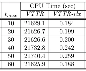
We compared theVTTRandVTTR-rlx on problem instances defined on a 16-node network. Recall that the VTTR subproblem of TG only takes into account the traffic demands {tsd} between nodes, not the physical topology of the network. We generated traffic instances by setting each traffic demand tsd as a random integer in the range [0, tmax]. We let parameter tmax = 10,20,30,40,50,60, and for each value of tmax we generated ten traffic matrices (i.e., problem instances) that were used to solve both VTTRand VTTR-rlx.

(32)

Table 2.1: CPU time comparison ofVTTR and VTTR-rlx,N = 16

CPU Time (sec) tmax VTTR VTTR-rlx

10 21629.1 0.184 20 21626.7 0.199 30 21626.6 0.200 40 21732.8 0.242 50 21740.4 0.259 60 21625.9 0.188

Table 2.2: Objective value comparison of VTTRand VTTR-rlx,N = 16

Objective Value (# of lightpaths)

VTTR VTTR-rlx

tmax (best available) (optimal) (rounded-up)

10 101.7 74.1 217.9

20 173.2 150.0 274.2

30 250.6 226.6 340.1

40 327.1 302.6 423.6

50 389.3 366.4 480.1

60 468.2 443.5 558.5

that the CPU times do not vary much across the values of tmax, but solving the partial LP relaxation VTTR-rlx takes a fraction of a second whereas solving the VTTR ILP takes longer than the six-hour limit we imposed.

Table 2.2 compares the best available solutions to VTTR obtained within the six-hour limit, to the optimal solutions to VTTR-rlx, in terms of the objective value (i.e., number of lightpaths). For each row of the table (i.e., a specific value of tmax), the values shown are averages over the corresponding ten traffic instances. However, the optimal solution to partial LP relaxation VTTR-rlx is a lower bound, but not necessarily a feasible solution to VTTR. Therefore, in the table we also present the objective value of the feasible solution obtained as described in Lemma 2.2.1, i.e., by rounding up the real values ¯b?_ij of the optimal solution to VTTR-rlx.

From the two tables we make two important observations. First, the integral constraints of the lightpath variables bij play an important role in increasing the complexity of the branch-and-bound process of the ILP solver. Second, rounding up the real lightpath values ¯b?

(33)

in a large optimality gap. Based on these observations, in the next section we develop three iterative algorithms that strike a good balance between running time and quality of solution.

2.2.2 Lightpath Utilization

Consider the optimal solution {¯b?_ij} to the VTTR-rlx problem and the corresponding feasible solution {d¯b?_ij e} toVTTR, obtained by rounding up all the lightpath variables. Let us define:

Uij =

¯

b?_ij

d¯b?_ije, ¯b ?

ij >0. (2.10)

The quantity Uij represents the utilization of the lightpaths from node i to node j in the rounded-up feasible solution. When the utilization is high (i.e., Uij is close to 1.0), the corre-sponding lightpath resources are used effectively in the solution; furthermore, rounding up the corresponding lightpath variable to obtain a feasible solution makes only a small contribution to the optimality gap. The opposite is true when the utilization of a set of lightpaths is low.

We now present three efficient algorithms based on partial LP relaxation and lightpath utilization in the following two subsections. The key idea of all the three algorithms is to treat the integer constraints on lightpath variablesbij aslazy constraints, and activate only a subset of them (or variants) at each utilization threshold setting.

2.2.3 VTTR-rlx(Uthr)

This iterative algorithm treats the integer constraints on lightpath variables bij as lazy con-straints, and activate only a subset of them at each iteration. Initially, we start by solving the partial LP relaxation VTTR-rlx in which none of the integrality constraints on{bij} are activated. If all lightpath variables in the optimal solution are integer, then this is a feasible (and optimal) solution to VTTR. Otherwise, we examine the solution to identify all lightpath variables ¯bij with a utilization Uij < uthr, where uthr is some threshold that is initialized to a small value, e.g., uthr = 0.1. We then activate the integrality constraints on the identified variables, i.e., we solve a modified version of VTTR-rlx in which the identified variables are replaced by integer variablesbij. We repeat this process, increasing the threshold valueuthrat each iteration, until one of the following stopping criteria is satisfied:

1. all lightpath variables in the solution are integer, and hence represent an optimal solution toVTTR;

2. the thresholduthr reaches a predetermined value1H ; or

1

Note that, if this predetermined upper boundH onuthr is 1.0, then the algorithm will continue until the

(34)

3. the improvement in the value of the objective function over the previous iteration is less than a predetermined minimum valueδ.

A combination of the above criteria may be used, e.g., stop whenever the threshold has reached a predetermined value or the improvement over the previous iteration is less thanδ, whichever is satisfied first.

This ascending utilizationVTTR(Uthr)iterative algorithm can be described by these steps: 1. Initialization: i←0;uthr←0.1.

2. Solve VTTR-rlx to obtain the optimal solution and determine the objective value Pi of the corresponding feasible solution obtained by rounding up all non-integer lightpath variables.

3. CalculateUij for all non-integer lightpaths in the optimal solution and modifyVTTR-rlx to activate the integrality constraints for the variables for which Uij ≤uthr.

4. If the stopping criterion is satisfied, return the current solution; otherwise set i ← i+ 1;uthr←uthr+ 0.1 and repeat from Step 2.

We note that, at each iteration of the algorithm, a tighter partial LP relaxation ofVTTRis considered, generally requiring longer time to solve. On the other hand, the objective value of the solution improves with each iteration. By selecting an appropriate stopping criterion, the iterative algorithm may be designed to deliver a desirable tradeoff between running time and quality of the final solution.

2.2.4 VTTR-rlx(Ul, Uh)

We define Ul and Uh, 0≤Ul ≤Uh ≤ 1, as low and high thresholds, respectively on lightpath utilization. We consider a modified version ofVTTR-rlx in whichbijis fixed todb

∗

ije, ifUij ≥Uh, and tobb∗_ijc, ifUij ≤Ul. In practice, the following two sets ofequality constraints are activated on the lightpath variables ¯bij with a utilizationUij ≤Ul orUij ≥Uh:

¯_b_ij ₌_d¯_b?

ije ∀ i, j: Uij ≥Uh (2.11)

¯

bij =b¯b?ijc ∀i, j: Uij ≤Ul (2.12) We letVTRL-rlx(Ul, Uh) denote the modified LP relaxation ofVTTRin which the variables ¯_b_ij _{are set to be equal to the floor (respectively, ceiling) of the corresponding optimal solution} obtained from VTTR-rlx ifUij ≤Ul (respectively,Uij ≥Uh).

last iteration. More practically, the upper bound onuthr should be strictly less but close to 1.0, e.g., H= 0.8.

(35)

The key idea behind the equality constraints (2.11) and (2.12) introduced in the formu-lation of VTRL-rlx(Ul, Uh) can be explained by using an airline analogy in which lightpaths corresponds to scheduled flights. For lightpaths with low utilization, constraint (2.12) forces the fractional lightpaths to zero; when solving the modified problem, the traffic carried by these fractional lightpath will be redirected to other lightpaths. In the airline analogy, this is equivalent to canceling flights that are close to empty. Note that the deletion of lightpaths (respectively, the canceling of flights) may cause some traffic (respectively, passengers) to take a longer route to their destination; however, from the point of view of network design, this may be an acceptable tradeoff if it leads to a smaller network cost. On the other hand, when lightpaths have high utilization, constraint (2.11) forces the fractional lightpath to become a full lightpath. As a result, the extra capacity of this new full lightpath becomes available to carry traffic that is potentially redirected by fractional lightpaths that were deleted.

The question that arises is how to determine the pair of thresholds (Ul, Uh), i.e., the specific partial LP relaxation of VTTR that provides a desired tradeoff between running time and quality of solution. To this end, we propose an iterative algorithm that uses a local search technique to select the pair (Ul, Uh). The iterative algorithm treats the integer constraints on lightpath variables{¯bij}aslazy constraints, activating only a subset of them at each iteration based on how they relate to the current pair of utilization thresholds.

The iterative algorithm starts by solving the partial LP relaxationVTTR-rlx in which none of the integrality constraints on {¯bij} are activated. If all lightpath variables in the optimal solution are integer, then this is a feasible (and optimal) solution to VTTR. Otherwise, the solution is examined to identify all lightpath variables with a utilizationUij outside the interval [Ul, Uh], and the corresponding VTRL-rlx(Ul, Uh) variant is solved. This process is repeated, increasing the threshold valueUl and decreasingUh at each iteration, until one of the following stopping criteria is satisfied:

1. all lightpath variables in the solution are integer, and hence represent an optimal solution toVTTR;

2. the threshold pair (Ul, Uh) reaches a predetermined value, or

3. the improvement in the value of the objective function over the previous iteration is less than a predetermined minimum valueδ.

A combination of the above criteria may be used, e.g., stop whenever the thresholds have reached a predetermined value or the improvement over the previous iteration is less than δ, whichever is satisfied first.

The iterative algorithm can be described by these steps:

(36)

2. SolveVTTR-rlx with no integer constraints on{¯bij} activated. Calculate and recordUij for all lightpath pairs in the optimal solution.

3. SolveVTTR-rlx(Ul, Uh). Find the new optimal solution, and determine the objective val-ue of the corresponding feasible solution obtained by rounding up all non-integer lightpath variables.

4. If the stopping criterion is satisfied, return the current solution; otherwise set Ul ← Ul+ 0.1; Uh←Uh−0.1 and repeat from Step 3.

We note that, at each iteration of the algorithm, a tighter partial LP relaxation of VTTR with a larger number of equality constraints is considered, generally requiring longer time to solve. On the other hand, the objective value of the solution improves with each iteration. By selecting an appropriate stopping criterion, especially in terms of the threshold values on lightpath utilization, this algorithm may be designed to deliver a desirable tradeoff between running time and quality of the final solution.

We note that, by imposing the two sets of equity constraints, we manually fix the value of bij, which may lead to the reduction of solution accuracy. However, it also strongly reduce the possible combinations involving thesebijs, which may highly reduce the corresponding running time. Thus, by running experiments, we aim to find a proper pair of (Ul, Uh) with the best solution quality in most cases.

2.2.5 VTTR-rlx(Ul, Uh)-Int

This algorithm is a variant of VTTR-rlx(Ul, Uh), such that, in addition to the two sets of equality constraints, we add one more set of integrality constraints.

1. In each iteration, the lightpath variablesbij withUl≤Uij ≤Uh are set to be integer, i.e., the type of ¯bij is changed from continuous to integral.

In the aspect of running time, by involving different numbers of integral constraints accord-ing to (Ul, Uh) value, the running time may have various increases. Thus, it will be useful to determine how many integral constraints to be added by choosing a proper pair of (Ul, Uh).

2.3 Numerical Results

(37)

Woodcrest Xeon CPU at 2.33GHz with 1333MHz memory bus, 4GB of memory and 4MB L2 cache.

Our study involves a large set of problem instances defined on several network sizes2 _with

various random traffic loads. In particular, we consider networks with N = 8, 16, 24, and 32 nodes. In all the simulations, we set the wavelength capacity C = 16. For each network topology, we consider several problem instances. For each problem instance, the traffic demand matrix T = [tsd] is generated by drawing the (integer) traffic demands uniformly at random in the interval [0, tmax]. The values of tmax we used in the simulations are 20, 30, 40, and 50. Each data point in the figures we present in this section represents the average of 10 random problem instances for the stated values of the input parameters.

Unless otherwise stated, we set the relative optimality gap to 2% for all CPLEX runs. Consequently, CPLEX terminates when it finds a solution that is within 2% of the optimal for the problem at hand, rather than continuing until the problem is solved to optimality. Later in this section we will investigate how the running time required to solve the VTTR problem is affected by this optimality gap.

2.3.1 VTTR-rlx(Uthr)

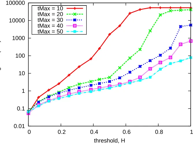
Figure 2.1 plots the running time of VTTR-rlx(Uthr) as a function of the threshold H. The algorithm runs until the threshold Uthr becomes equal to H, and this is used as the only stopping criterion. Note that, whenH= 0, only the partial LP relaxation VTTR-rlx is solved, whereas when H= 1, the fullVTTR problem is solved; for values ofH between zero and one, intermediate versions ofVTTR-rlx are solved whereby integrality constraints are imposed only on lightpath variables with utilization less than H, as we discussed in the previous section. The figure plots results for networks with N = 12 and various values of tmax. As expected, the running time increases as H increases, since larger values of H imply that the integrality constraints are impsoed on a larger number of lightpath variables. We also see that the running time is affected by the value of parameter tmax. As tmax increases, the overall traffic to the network increases as well, a larger number of lightpaths need to be established to carry the traffic, hence the optimal objective value is higher. Consequently, an optimality gap of 2% translates to a larger absolute difference (in the number of lightpaths) from the optimal objective value astmax increases; in turn, CPLEX reaches this lower value faster.

For the remainder of the experiments in this section, we present results for problem instances withtmax= 30. With this value oftmax, the average size of demands between source-destination pairs is close to the capacity C= 16 of a wavelength. Results for other values of tmax exhibit the same behavior and are omitted.

(38)

0.01 0.1 1 10 100 1000 10000 100000

0 0.2 0.4 0.6 0.8 1

Running time (sec)

threshold, H tMax = 10

tMax = 20 tMax = 30 tMax = 40 tMax = 50

Figure 2.1: CPU time, as a function of H,N = 12, iterative algorithm VTTR-rlx(Uthr)

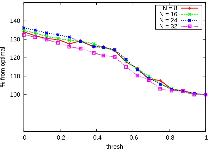
Figure 2.2 plots the quality of the solution of the iterative algorithm as a function of the thresholdHand for various network sizes. The quality of the solution for a given value ofH is expressed as:

P

d¯b? ije

P

b?_ij , (2.13)

where the numerator is the feasible solution toVTTRobtained by rounding up the lightpath variables in the optimal solution to the VTTR-rlx problem for the given value of H, whileb?_ij is the optimal solution to the VTTR problem (i.e., whenH = 1). As expected, the quality of the solution starts high whenH = 0 (i.e., all integer lightpaths are relaxed) and then decreases until it reaches optimality for H = 1. Importantly, for all network sizes shown in the figure, the solution is within 5% of the optimal as soon as H = 0.8. As we remarked earlier, such a value for H ensures that all wavelengths are highly utilized while also making it possible to accommodate future demands without necessarily setting up additional lightpaths.

(39)

100 110 120 130 140

0 0.2 0.4 0.6 0.8 1

% from optimal

thresh

N = 8 N = 16 N = 24 N = 32

Figure 2.2: Quality of solution as a function of H, algorithm VTTR-rlx(Uthr), tmax = 30

much in terms of optimality (as Figure 2.2 indicates). Such problem instances are impossible to solve using the original formulation for the TG problem.

2.3.2 VTTR-rlx(Ul, Uh)

Solution Quality

Figure 2.4 plots the quality of the solution of VTTR-rlx(Ul, Uh) as a function of the pair of thresholds (Ul, Uh) and for various network sizes. The quality of the solution is defined similarly as:

P

ijd¯b?ije

P

ijb?ij

. (2.14)

The numerator in this expression is the value of the feasible solution to VTTR obtained by rounding up the lightpath variables in the optimal solution to the modified version of VTTR-rlx(Ul, Uh) problem for the given value of a pair of thresholds. The denominator is the value of the objective function for the optimal solution to theVTTRproblem (obtained within a 2% relative optimality gap, as we explained earlier). A low value of the above expression denotes a higher solution quality.

(40)

0.01 0.1 1 10 100 1000 10000 100000

8 16 24 32

Running time (sec)

N H = 0.8

Figure 2.3: CPU time as a function ofN, iterative algorithmVTTR-rlx(Uthr),H= 0.8, tmax= 30

point (0,0) in the figure) since all integer lightpath variables are relaxed; the solution quality then improves asUlincreases orUh decreases. The best result is achieved for the threshold pair (Ul, Uh) = (0.5,0.6). Importantly, for all network sizes shown in the figure, the solution is about 11% from the optimal one as soon as (Ul, Uh) = (0.5,0.6); this worst case occurs forN = 8, and the gap decreases as the network sizeN increases. For the 32-node network, the gap is as small as 3%. Note that this pair of values for (Ul, Uh) ensures that no wavelength is under-utilized (i.e., it is filled to 50% at minimum) while also leaving some room to accommodate future demands without necessarily setting up additional lightpaths.

Scalability

(41)

1.0 1.1 1.2 1.3 1.4

(0,0) (0.1,0.9) (0.2,0.9) (0.3,0.9) (0.4,0.9) (0.5,0.9) (0.1,0.8) (0.2,0.8) (0.3,0.8) (0.4,0.8) (0.5,0.8) (0.1,0.7) (0.2,0.7) (0.3,0.7) (0.4,0.7) (0.5,0.7) (0.1,0.6) (0.2,0.6) (0.3,0.6) (0.4,0.6) (0.5,0.6)

solution quality

(Ul, Uh)

N=8 N=16 N=24 N=32

Figure 2.4: Solution quality as a function of (Ul, Uh),tmax= 30

few seconds. This shows that the algorithm is effective across a range of traffic loads.

Based on the last observation, for the simulations in the remainder of this section we have fixed the value of tmax= 30; with this value oftmax, the average size of demands between any source-destination pair is close to the capacityC = 16 of a wavelength. Results for other values of tmax exhibit the same behavior and are omitted.

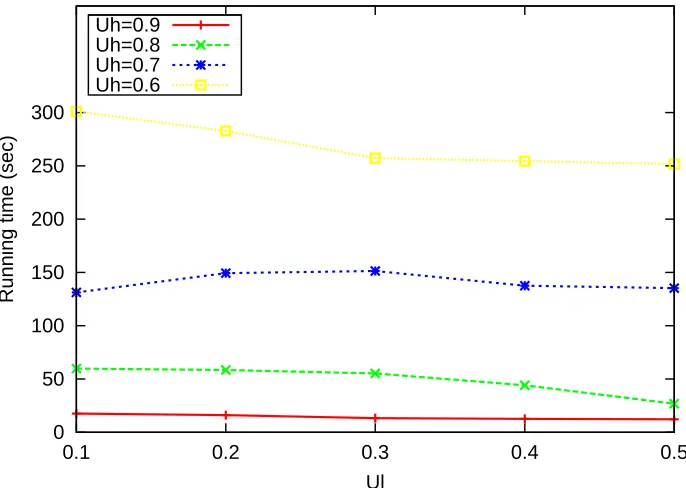
Figure 2.6 plots the CPU time to solve VTTR-rlx(Ul, Uh) as a function of Ul. We plot results for a 24-node network, as they are representative of the running time trends for other network sizes. As shown in the figure, whenUh is kept fixed, the running time does not change significantly as a function of the lower threshold valueUl. However, asUhdecreases, the running time increases significantly. In other words, the value of the high threshold Uh has a stronger influence on the performance of the algorithm with respect to running time.

(42)

0.1 1 10

(0,0) (0.1,0.9) (0.2,0.9) (0.3,0.9) (0.4,0.9) (0.5,0.9) (0.1,0.8) (0.2,0.8) (0.3,0.8) (0.4,0.8) (0.5,0.8) (0.1,0.7) (0.2,0.7) (0.3,0.7) (0.4,0.7) (0.5,0.7) (0.1,0.6) (0.2,0.6) (0.3,0.6) (0.4,0.6) (0.5,0.6)

running time in sec

(Ul, Uh)

tmax=20 tmax=30 tmax=40 tmax=50

Figure 2.5: CPU time as a function of (Ul, Uh), N = 16

Finally, Figure 2.8 compares the running time as a function of network size of three methods for solving theVTTR problem:

1. solvingVTTR to optimality;

2. solvingVTTR with a 2% relative optimality gap; and

3. solvingVTTR-rlx(0.5,0.6) with a 2% relative optimality gap.

(43)

0 50 100 150 200 250 300

0.1 0.2 0.3 0.4 0.5

Running time (sec)

Ul Uh=0.9

Uh=0.8 Uh=0.7 Uh=0.6

Figure 2.6: CPU time as a function ofUl,N = 24, tmax=30

is 2% from the optimal solution as the network size increases, as the absolute difference from the optimal solution is larger. Of course, as the network size increases further, the increase in the number of variables and constraints becomes once again the factor determining the running time; hence the increase as network size grows to 24 and beyond.

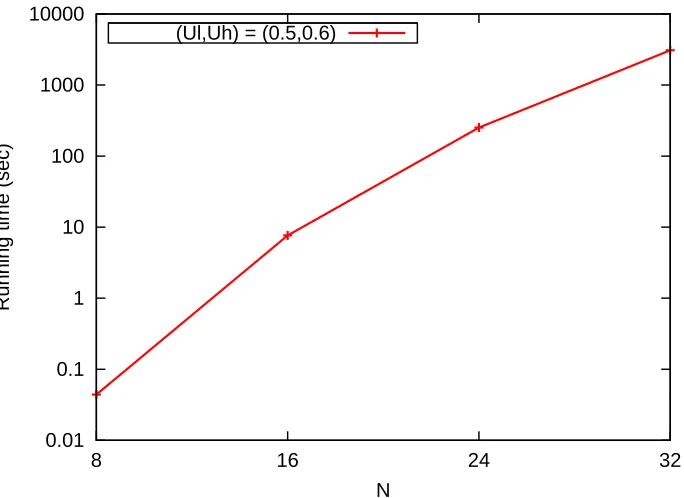
Finally, solving the modified VTTR-rlx(Ul, Uh) relaxed problem is significantly faster over all network sizes, and reduces the running time by more than one order of magnitude compared to solving VTTR directly within a 2% optimality gap. In particular, the VTTR-rlx(Ul, Uh) problem can be solved on the 32-node network in about 3000 seconds (i.e., less than one hour), while also obtaining a solution that is within 3% of the best solution (refer also to Figure 2.4) that we were able to obtain after running the second method for 24 hours. Note that in Figure 2.8, we used (Ul, Uh) = (0.5,0.6) as the pair of thresholds for the algorithm; however, depending on the relative importance of solution quality to running time, other pairs of thresholds may be applied to further reduce the running time (as shown in Figure 2.6).

(44)

0.01 0.1 1 10 100 1000 10000

8 16 24 32

Running time (sec)

N (Ul,Uh) = (0.5,0.6)

Figure 2.7: CPU time as a function ofN, (Ul, Uh) = (0.5,0.6), tmax= 30

2.3.3 VTTR-rlx(Ul, Uh)-Int

In Fig. 2.9, it plots the quality of solution against pairs of various threshold values for 8-, 16- and 24-node networks with tmax = 30, where Ul = 0.3,0.4,0.5 and Uh = 0.6,0.7,0.8. The quality of solution is defined similarly as in the previous subsection. A close to 1.0 value indicates a high solution quality. First, generally, when Uh is fixed, the solution quality is higher when Ul decreases; when Ul is fixed, the solution quality is higher when Uh increases. In other words, the more integrality constraints are, the better the quality of solution is. Unlike the VTTR-rlx(Ul, Uh) algorithm, for all the three network sizes, the most extreme threshold pair (Ul, Uh) = (0.3,0.8) provides the best solution quality (very close to 1.0). This can be explained as when (Ul, Uh) = (0.3,0.8), the most integrality constraints are present, hence it is the closest to the original VTTR problem. Second, the solution quality is more sensitive toUl, i.e., as long asUl remains low (=0.3), we have good solution quality within 3% of the best objective value obtained from solving VTTR with 2% optimality gap.

(45)

0.01 0.1 1 10 100 1000 10000 time limit

8 16 24 32

Running time (sec)

N

VTTR (solved to optimality) VTTR (solved with 2% gap) Iterative algorithm (solved with 2% gap)

Figure 2.8: CPU time comparison as a function of network sizeN,tmax= 30

and 2.10, we can use (Ul, Uh) = (0.3,0.8) for all the three network sizes in order to obtain a good tradeoff between solution quality and running time. Depending on the practical needs, we may also choose different pairs of (Ul, Uh) values. For example, (0.3,0.6) can be used to obtain a one order of magnitude decrease in running time for 8-node network.

2.3.4 Wavelength Fragmentation

(46)

1.0 1.1 1.2 1.3 1.4

(0,0) (0.5,0.6) (0.4,0.6) (0.3,0.6) (0.5,0.7) (0.4,0.7) (0.3,0.7) (0.5,0.8) (0.4,0.8) (0.3,0.8)

solution quality

(Ul, Uh)

N=8 N=16 N=24

Figure 2.9: Solution Quality forVTTR-rlx(Ul, Uh)-Int, N=8, 16, 24, tmax=30

0.01 0.1 1 10 100 1000 10000

(0,0) (0.5,0.6) (0.4,0.6) (0.3,0.6) (0.5,0.7) (0.4,0.7) (0.3,0.7) (0.5,0.8) (0.4,0.8) (0.3,0.8)

CPU time in sec

(Ul, Uh)

N=8 N=16 N=24

(47)

1 2 3 4 5 2

4 6 8 10 12 14 16 18 20 22

Traffic Instance

Number of wavelength used

Sequential TG, W=5

TG, W=10

TG, W=30

(48)

Chapter 3

Hierarchical Virtual Topology and

Traffic Routing

As we mentioned earlier, the ILP formulation presented in Chapter 1 serves as the basis for reasoning about and tackling the traffic grooming problem. Unfortunately, as we have seen from Chapter 1, solving the ILP formulation directly does not scale to instances with more than a handful of nodes, and cannot be applied to networks of practical size covering a national or international geographical area. Based on this observation, in Chapter 2, we have presented a novel decomposition of traffic grooming problem on general topologies, which consists of two sequential subproblems - the VTTR and RWA subproblems. We have also developed three efficient heuristic algorithms for the VTTR subproblem to obtain a good tradeoff between solution quality and running time.

These studies regard the network as a flat entity for the purpose of traffic grooming. How-ever, it is well-known that existing networks resources are typically managed and controlled in a hierarchical manner. The levels of the hierarchy either reflect the underlying organiza-tional structure of the network or are designed in order to ensure scalability of the control and management functions. Accordingly, several studies have adopted a variety of hierarchical approaches to traffic grooming that, by virtue of decomposing the network, scale well and are more compatible with the manner in which networks operate in practice.

(49)

3.1 Related Work in Hierarchical Grooming

3.1.1 Ring Networks

Early research in traffic grooming focused on ring topologies [17], [38], [13], mainly due to the practical importance of upgrading the existing SONET/SDH infrastructure to support multiple wavelengths. A point-to-point WDM ring is a straightforward extension of a SONET/SDH network, but requires that each node be equipped with one add-drop multiplexer (ADM) per wavelength. Clearly, such a solution has a high ADM cost and cannot scale to more than a few wavelengths. Therefore, much of the research in this context has been on reducing the number of ADMs by grooming sub-wavelength traffic onto lightpaths that optically bypass intermediate nodes, and several near-optimal algorithms have been proposed in [13,38]. However, approaches that do not impose a hierarchical structure on the ring network may produce traffic grooming solutions, in terms of the number of ADMs and their placement, that can be sensitive to the input traffic demands.

The study in [17] was the first to present several hierarchical ring architectures and to characterize their cost in terms of the number of ADMs (equivalently, electronic transceivers or ports) and wavelengths for non-blocking operation under a model of dynamic traffic. In a single-hub ring architecture, each node is directly connected to the single-hub by a number of lightpaths, and all traffic between non-hub nodes goes through the hub. In a double-hub architecture, there are two hub nodes diametrically opposite to each other in the ring. Each node is connected to both hubs by direct lightpaths, and non-hub nodes send their traffic to the hubs for grooming and forwarding to the actual destination.

A more general hierarchical ring architecture was also proposed in [17]. In this architecture, shown in Figure 3.1, ring nodes are partitioned into two types: access andbackbone. The set of wavelengths is also partitioned into access and backbone wavelengths. The access wavelengths are used to connect all nodes, including access and backbone nodes, in a point-to-point WDM ring that forms the first level of the hierarchy. At the second level of the hierarchy, the backbone wavelengths are used to form a point-to-point WDM ring among the backbone nodes only. This hierarchy determines the routing of traffic between two access nodes as follows. If the two access nodes are such that there is no backbone node along the shortest path between them, their traffic is routed using single-hop lightpaths over the access ring along the shortest path. Otherwise, suppose that b1 and b2 are the first and last backbone nodes, respectively, along the shortest

path between two access nodes a1 and a2 (note that b1 and b2 may coincide). Then, traffic

froma1 toa2 is routed to b1 over the access ring, from there tob2 over the backbone ring, and

finally over the access ring to a2.