GMM E
STIMATION WITH
P
ERSISTENT
P
ANEL
D
ATA
:
A
N
A
PPLICATION TO
P
RODUCTION
F
UNCTIONS
GMM estimation with persistent panel data:
an application to production functions
Richard Blundell
University College London and Institute for Fiscal Studies
Stephen Bond
Nu¢eld College, Oxford and Institute for Fiscal Studies
September 1998
Paper presented at the Eighth International Conference on Panel Data
Göteborg University, June 11-12, 1998
JEL classi…cation: C23, D24
Summary
We consider the estimation of Cobb-Douglas production functions using panel data covering a large sample of companies observed for a small number of time periods. Standard GMM estimators, which eliminate unobserved …rm-speci…c e¤ects by taking …rst di¤erences, have been found to produce unsatisfactory results in this context (Mairesse and Hall, 1996).
We attribute this to weak instruments: the series on …rm sales, capital and employment are highly persistent, so that lagged levels are only weakly correlated with subsequent …rst di¤erences. As shown in Blundell and Bond (1998), this can result in large …nite-sample biases when using the standard …rst-di¤erenced GMM estimator.
Blundell and Bond (1998) also show that these biases can be dramatically reduced by exploiting reasonable stationarity restrictions on the initial conditions process. This yields an extended GMM estimator in which lagged …rst-diferences of the series are also used as instruments for the levels equations (cf. Arellano and Bover, 1995).
“In empirical practice, the application of panel methods to micro-data produced rather unsatisfactory results: low and often insigni…cant cap-ital coe¢cients and unreasonably low estimates of returns to scale.”
— Griliches and Mairesse (1997).
1. Introduction
lagged …rst-di¤erences as instruments for equations in levels, in addition to the usual lagged levels as instruments for equations in …rst-di¤erences (cf. Arellano and Bover, 1995).
2. Model
We consider the Cobb-Douglas production function
yit =¯nnit+¯kkit+°t+ (´i+vit+mit) (2.1)
vit =½vi;t¡1+eit j½j<1
eit; mit sM A(0)
whereyitis log sales of …rm i in year t,nitis log employment,kitis log capital stock
and °t is a year-speci…c intercept. Of the error components, ´i is an unobserved
…rm-speci…c e¤ect, vit is a possibly autoregressive (productivity) shock and mit
re‡ects serially uncorrelated measurement errors. Constant returns to scale would
imply ¯n+¯k = 1, but this is not necessarily imposed.
We are interested in consistent estimation of the parameters (¯n; ¯k; ½) when
the number of …rms(N)is large and the number of years(T)is …xed. We maintain
that both employment (nit) and capital (kit) are potentially correlated with the
…rm-speci…c e¤ects(´i), and with both productivity shocks(eit)and measurement
errors (mit):
The model has a dynamic (common factor) representation
yit = ¯nnit¡½¯nni;t¡1+¯kkit¡½¯kki;t¡1+½yi;t¡1 (2.2)
+(°t¡½°t¡1) + (´i(1¡½) +eit+mit¡½mi;t¡1)
or
yit =¼1nit+¼2ni;t¡1+¼3kit+¼4ki;t¡1+¼5yi;t¡1+°t¤ + (´¤i +wit) (2.3)
subject to two non-linear (common factor) restrictions ¼2 = ¡¼1¼5 and ¼4 =
(¼1; ¼2; ¼3; ¼4; ¼5)andvar(¼), these restrictions can be (tested and) imposed using
minimum distance to obtain the restricted parameter vector (¯n; ¯k; ½). Notice
that wit = eit s MA(0) if there are no measurement errors (var(mit) = 0), and
wits MA(1) otherwise.
3. GMM estimation
3.1. First di¤erences
A standard assumption on the initial conditions (E[xi1eit] = E[xi1mit] = 0 for t = 2; :::; T) yields the following moment conditions
E[xi;t¡s¢wit] = 0 wherexit = (nit; kit; yit) (3.1)
for s >2 when wit sMA(0), and for s >3 when wit s MA(1). This allows the
use of suitably lagged levels of the variables as instruments, after the equation has been …rst-di¤erenced to eliminate the …rm-speci…c e¤ects (cf. Arellano and Bond, 1991).
Note however that the resulting …rst-di¤erenced GMM estimator has been found to have poor …nite sample properties (bias and imprecision) when the lagged levels of the series are only weakly correlated with subsequent …rst di¤erences, so that the instruments available for the …rst-di¤erenced equations are weak (cf. Blundell and Bond, 1998). This may arise here when the marginal processes for
employment (nit) and capital(kit) are highly persistent, or close to random walk
processes, as is often found to be the case.
To be more precise about these statements, consider the AR(1) model
yit =®yi;t¡1+´i+vit (3.2)
where vit here is serially uncorrelated (½= 0). The instruments used in the
stan-dard …rst-di¤erenced GMM estimator become less informative in two important
unity; and second, as the variance of the permanent e¤ects (´i) increases relative to the variance of the transitory shocks (vit). For simplicity, consider the case with
T = 3: In this case, the moment conditions corresponding to the …rst-di¤erenced
GMM estimator reduce to a single orthogonality condition. The …rst-di¤erenced GMM estimator estimator then corresponds to a simple instrumental variable (IV) estimator with reduced form (instrumental variable regression) equation
¢yi2 =¼yi1+ri for i= 1; ::::; N: (3.3)
For su¢ciently high autoregressive parameter®or for su¢ciently high variance
of the permanent e¤ects, the least squares estimate of the reduced form coe¢cient
¼ can be made arbitrarily close to zero. In this case the instrument yi1 is only
weakly correlated with ¢yi2: To see this notice that the model (3.2) implies that
¢yi2 = (®¡1)yi1+´i+vi2 for i= 1; ::::; N: (3.4)
The least squares estimator of(®¡1)in (3.4) is generally biased upwards, towards
zero, since we expectE(yi1´i)>0:Assuming stationarity and letting¾2´ = var(´i)
and ¾2
v = var(vit), the plim of b¼ is given by
plimb¼= (®¡1)¾2 k ´
¾2 v +k
with k = (1¡®)
2
(1¡®2):
The bias term e¤ectively scales the estimated coe¢cient on the instrumental
vari-able yi1 toward zero. We …nd that plim¼b ! 0 as ® ! 1 or as (¾2´=¾2v) ! 1,
which are the cases in which the …rst stage F-statistic is Op(1).
Blundell and Bond (1998) characterise this problem of weak instruments using the concentration parameter of Nelson and Startz (1990a,b) and Staiger and Stock (1997). First note that the F-statistic for the …rst stage instrumental variable regression converges to a noncentral chi-squared with one degree of freedom. The concentration parameter is then the corresponding noncentrality parameter which
stationarity,¿ has the following simple characterisation in terms of the parameters of the AR(1) model
¿ = (¾
2
vk)2
¾2
´ +¾2vk
where k = (1¡®)
2
(1¡®2): (3.5)
The performance of the …rst-di¤erenced GMM estimator in this AR(1)
speci…ca-tion can therefore be seen to deteriorate as® !1, as well as for increassing values
of (¾2
´=¾2v).
Blundell and Bond (1998) also report some results of a Monte Carlo study which investigates the …nite sample properties of these GMM estimators in the AR(1) model. In Table 1 we present some speci…c examples that highlight the
issues involved. We consider sample sizes withN = 100and500,T = 4and values
for ® of 0.5, 0.8 and 0.9. In all cases reported here, ¾2
´ = ¾2v = 1 and the initial
conditions yi1 satisfy stationarity. These results illustrate the poor performance
of the …rst-di¤erenced GMM estimator (DIF) at high values of®. Table 1 column
‘DIF’ presents the mean and standard deviation for this estimator in the Monte
Carlo simulations. Consider the experiments where ® is 0.8 or 0.9. For the
…rst-di¤erenced GMM estimator we …nd both a huge downward bias and very imprecise estimates. This is consistent with our analysis of weak instruments. For this reason, we consider further restrictions on the model which may yield more informative moment conditions.
3.2. Levels
If we are willing to assume that E[¢nit´¤i] = E[¢kit´i¤] = 0 and that the initial conditions satisfy E[¢yi2´¤i] = 0, then we obtain the additional moment conditions
for s = 1 when wit s M A(0), and for s = 2 when wit s M A(1) (cf. Arellano
and Bover, 1995).1 This allows the use of suitably lagged …rst di¤erences of
the variables as instruments for the equations in levels. Both sets of moment conditions can be exploited as a linear GMM estimator in a system containing both …rst-di¤erenced and levels equations. Combining both sets of moment conditions provides what we label the system (SYS) GMM estimator.
For the AR(1) model, Table 1 shows that there can be dramatic reductions in …nite sample bias from exploiting additional moment conditions of this type, in cases where the autoregressive parameter is only weakly identi…ed from the …rst-di¤erenced equations. This can also result in substantial improvements in precision. In contrast to the DIF estimator, there is virtually no bias and much
better precision, even in the smaller sample size and for ® of order 0.8.
3.3. Validity of the levels restrictions
To consider when these additional assumptions are likely to be valid in a multivariate context, we brie‡y consider the model
yit =®yi;t¡1+¯xit+ (´i+eit) (3.7)
and close this by considering the following AR(1) process for the regressor
xit =°xi;t¡1+ (±´i+uit): (3.8)
Thus ± > 0 allows the level of xit to be correlated with ´i, and we also allow
E[uiteit]6= 0.
First notice that by repeated substitution after …rst-di¤erencing (3.8), we can write
¢xit =°t¡2¢xi2+
t¡3
X
s=0
°s¢ui;t¡s (3.9)
1Further lagged di¤erences can be shown to be redundant if all available moment conditions
so that ¢xit will be correlated with´i if and only if ¢xi2 is correlated with´i. To guarantee E[¢xi2´i] = 0 we require the initial conditions restriction
E
·µ
xi1¡
±´i
1¡°
¶
±´i
¸
= 0 (3.10)
which would be satis…ed under stationarity of the xit process.
Given this restriction, writing¢yit similarly as
¢yit =®t¡2¢yi2+
t¡3
X
s=0
®s(¯¢x
i;t¡s+ ¢ei;t¡s) (3.11)
shows that ¢yit will be correlated with ´i if and only if ¢yi2 is correlated with
´i. To guarantee E[¢yi2´i] = 0 we then require the similar initial conditions
restriction
E
2 4
0 @yi1¡
¯³±´i
1¡°
´
+´i
1¡®
1 A´i
3
5= 0 (3.12)
which would again be satis…ed under stationarity. Thus joint stationarity of theyit
and xit processes is su¢cient (but not necessary) for the validity of the additional
moment restrictions for the equations in levels. The moment conditions (3.6) thus require the …rst moments of (nit; kit; yit)to be time-invariant (conditional on common year dummies), but do not restrict the second and higher order moments of the series.
4. Data
5. Results
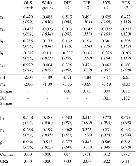
5.1. Basic production function estimates
Table 2 reports results for the basic production function, not imposing con-stant returns to scale, for a range of estimators. We report results for both the unrestricted model (2.3) and the restricted model (2.1), where the common factor
restrictions are tested and imposed using minimum distance.2 We report results
for a one-step GMM estimator, for which inference based on the asymptotic vari-ance matrix has been found to be more reliable than for the (asymptotically) more e¢cient two-step estimator. Simulations suggest that the loss in precision that results from not using the optimal weight matrix is unlikely to be large (cf. Blundell and Bond, 1998).
As expected in the presence of …rm-speci…c e¤ects, OLS levels appears to give an upwards-biased estimate of the coe¢cient on the lagged dependent variable, whilst within groups appears to give a downwards-biased estimate of this
coe¢-cient. Note that even using OLS, we reject the hypothesis that ½ = 1, and even
using within groups we reject the hypothesis that ½= 0: Although the pattern of
signs on current and lagged regressors in the unrestricted models are consistent with the AR(1) error-component speci…cation, the common factor restrictions are
rejected for both these estimators. They also reject constant returns to scale.3
The validity of lagged levels dated t-2 as instruments in the …rst-di¤erenced
equations is clearly rejected by the Sargan test of overidentifying restrictions.4
This is consistent with the presence of measurement errors. Instruments dated t-3 (and earlier) are accepted, and the test of common factor restrictions is easily passed in these …rst-di¤erenced GMM results. However the estimated coe¢cient
2The unrestricted results are computed using DPD98 for GAUSS (see Arellano and Bond,
1998).
3The table reports p-values from minimum distance and Wald tests of these parameter
restrictions.
on the lagged dependent variable is barely higher than the within groups estimate. We expect this coe¢cient to be biased downwards if the instruments available are weak (cf. Blundell and Bond (1998) and Table 1). Indeed the di¤erenced GMM parameter estimates are all very close to the within groups results. The estimate
of ¯k is low and statistically weak, and the constant returns to scale restriction is
rejected.
The validity of lagged levels dated t-3 (and earlier) as instruments in the …rst-di¤erenced equations, combined with lagged …rst di¤erences dated t-2 as instruments in the levels equations, appears to be marginal in the system GMM estimator. However this is partly re‡ecting the increased power of the Sargan test to reject the instruments used in the …rst-di¤erenced equations. A Di¤erence-Sargan statistic that speci…cally tests the additional moment conditions used in the levels equations accepts their validity at the 10% level. The system GMM parameter estimatates appear to be reasonable. The estimated coe¢cient on the lagged dependent variable is higher than the within groups estimate, but well below the OLS levels estimate. The common factor restrictions are easily
accepted, and the estimate of ¯k is both higher and better determined than the
di¤erenced GMM estimate. The constant returns to scale restriction is easily
accepted in the system GMM results.5
5.2. Diagnosis
If the system GMM results are to be our preferred parameter estimates, we have to explain why the di¤erenced GMM results should be biased. If the in-struments used in the …rst-di¤erenced estimator are weak, then the di¤erenced
GMM results are expected to be biased in the direction of within groups. Note
5One puzzle is that we …nd little evidence of second-order serial correlation in the
…rst-di¤erenced residuals (i.e. an M A(1) component in the error term in levels), although the use
of instruments dated t-2 is strongly rejected. It may be that the eit productivity shocks are
that the …rst-di¤erenced (one-step) GMM estimator coincides with a 2SLS es-timator, exploiting the same moment conditions, when the …rm-speci…c e¤ects are eliminated using the orthogonal deviations transformation, rather than tak-ing …rst-di¤erences (Arellano and Bover, 1995). Note also that OLS in the model transformed to orthogonal deviations coincides with within groups (Arellano and Bover, 1995), and that weak instruments will bias 2SLS in the direction of OLS (Nelson and Startz, 1990a,b). Hence weak instruments will bias this particular 2SLS estimator (which coincides with …rst-di¤erenced GMM) in the direction of within groups. Thus the similarity between our di¤erenced GMM and within groups results suggests that weak-instruments biases may be important here.
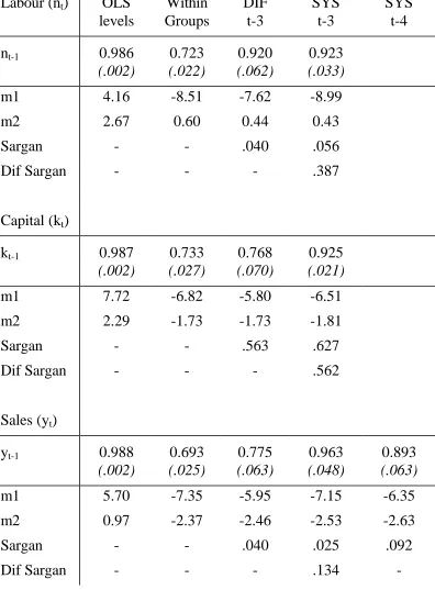
To investigate this further, Table 3 reports simple AR(1) speci…cations for the three series, employment (nit), capital (kit) and sales (yit). All three series are found to be highly persistent, although even using OLS levels estimates none is found to have an exact unit root. For the employment series, both di¤erenced and system GMM estimators suggest an autoregressive coe¢cient around 0.9, and di¤erenced GMM does not appear to be seriously biased. However for capital and sales, whilst system GMM again suggests an autoregressive coe¢cient around 0.9, the di¤erenced GMM estimates are found to be signi…cantly lower, and close to the corresponding within groups estimates. These downward biases in di¤erenced GMM estimates of the AR(1) models for capital and sales are consistent with the …nite sample biases found in Blundell and Bond (1998) and illustrated in Table 1. Indeed the surprise is that di¤erenced GMM gives reasonable results for the employment series. One di¤erence is that the variance of the …rm-speci…c e¤ects is found to be lower, relative to the variance of transitory shocks, for the employment series. The ratio of these variances is around 1.2 for employment, but 2.2 for capital and 1.7 for sales.
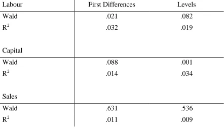
instruments is available. The reduced form regression for the …rst-di¤erenced
estimator relates ¢xi;88 to xi;86 and further lags. These instruments are jointly
signi…cant in the employment reduced form, but not for capital or sales. This helps to explain why the di¤erenced GMM estimator performs poorly in the models for capital and sales. The reduced form regression for the levels equations relates
xi;88 to ¢xi;87 and further lags. These instruments are jointly signi…cant in the
capital reduced form, although not for sales. This helps to explain why the system GMM estimator, which exploits both sets of moment conditions, works well for the capital series.
These results suggest that weak instruments biases are a potential problem when relying on …rst-di¤erenced GMM estimators using these persistent series. This does not necessarily imply that weak instruments will be a problem when estimating the production function, since it may be that lagged combinations of the three series will be more informative than the lagged levels of any one series alone. However our results in Table 2 suggest that there may be important …nite sample biases a¤ecting the di¤erenced GMM estimates of the production function. Moreover it is no surprise that the largest biases appear to be found on the coe¢cients for capital and lagged sales.
5.3. Constant returns to scale
Our preferred system GMM results in Table 2 accept the validity of the con-stant returns to scale restriction. Table 5 considers imposing this restriction using each of the estimators. Two points are noteworthy. First, the validity of the mo-ment conditions used to obtain the system GMM estimates becomes less marginal after imposing constant returns to scale. However the parameter estimates are very close to those found in Table 2, and the common factor restriction continues to hold.
GMM results, and not so close to the within groups estimates. Imposing constant returns to scale here seems to reduce the weak instruments biases in the di¤erenced
GMM estimates, possibly because the capital-labour ratio is less persistent than
the levels of either series. This may provide some justi…cation for the practice of imposing constant returns to scale in order to obtain reasonable estimates of the coe¢cient on capital, even though the restriction tends to be rejected with …rst-di¤erenced estimators.
Both these points increase our con…dence that the system GMM estimator works well in this application.
6. Conclusions
In this paper we have considered the estimation of a simple Cobb-Douglas produc-tion funcproduc-tion using an 8 year panel for 509 R&D-performing US manufacturing companies. Our …ndings suggest the importance of …nite-sample biases due to weak instruments when the …rst-di¤erenced GMM estimator is used, although these biases appear less important when constant returns to scale is imposed. We obtain much more reasonable results using the system GMM estimator: speci…-cally we …nd a higher and strongly signi…cant capital coe¢cient, and we do not reject constant returns to scale. We …nd that the additional instruments used in the system GMM estimator are both valid and informative in this context.
re-ducing …nite-sample biases associated with …rst-di¤erenced GMM.
References
[1] Arellano, M. and S.R. Bond (1991), Some tests of speci…cation for panel data:
Monte Carlo evidence and an application to employment equations, Review
of Economic Studies, 58, 277-297.
[2] Arellano, M. and S.R. Bond (1998), Dynamic Panel Data Estimation using DPD98 for GAUSS, mimeo, Institute for Fiscal Studies, London.
[3] Arellano, M. and O. Bover (1995), Another look at the instrumental-variable
estimation of error-components models, Journal of Econometrics, 68, 29-52.
[4] Blundell, R.W. and S.R. Bond (1998), Initial Conditions and Moment
Re-strictions in Dynamic Panel Data Models, Journal of Econometrics, 87,
115-143.
[5] Bond, S.R., D. Harho¤ and J. Van Reenen (1998a), R&D and Productivity in Germany and the United Kingdom, mimeo, Institute for Fiscal Studies, London.
[6] Bond, S.R., D. Harho¤ and J. Van Reenen (1998b), Investment, R&D and Financial Constraints in Britain and Germany, mimeo, Institute for Fiscal Studies, London.
[7] Bond, S.R., A. Hoe-er and J. Temple (1998), GMM Estimation of Empirical Growth Models, mimeo, Nu¢eld College, Oxford.
[8] Griliches, Z. and J. Mairesse (1997), Production Functions: the Search for
Identi…cation, forthcoming in S. Strom (ed.), Essays in Honour of Ragnar
[9] Mairesse, J. and B.H. Hall (1996), Estimating the Productivity of Research and Development in French and US Manufacturing Firms: an Exploration of Simultaneity Issues with GMM Methods, in Wagner, K. and B. Van Ark
(eds.), International Productivity Di¤erences and Their Explanations,
Else-vier Science, 285-315.
[10] Nelson, C.R. and R. Startz (1990a), Some Further Results on the Exact Small
Sample Properties of the Instrumental Variable Estimator, Econometrica, 58,
967-976.
[11] Nelson, C.R. and R. Startz (1990b), The Distribution of the Instrumental
Variable Estimator and its t-ratio When the Instrument is a Poor One,
Jour-nal of Business Economics and Statistics, 63, 5125-5140.
[12] Staiger, D. and J.H. Stock (1997), Instrumental Variables Regression with