Least angle regression for time series forecasting with
many predictors
Sarah Gelper and Christophe Croux
DEPARTMENT OF DECISION SCIENCES AND INFORMATION MANAGEMENT (KBI)
Least Angle Regression for Time Series Forecasting
with Many Predictors
Sarah Gelper and Christophe Croux
Faculty of Business and Economics, Katholieke Universiteit Leuven, Naamsestraat 69, 3000 Leuven, Belgium.
Abstract: Least Angle Regression (LARS) is a variable selection method with proven performance for cross-sectional data. In this paper, it is extended to time series forecasting with many predictors. The new method builds parsimonious fore-cast models, taking the time series dynamics into account. It is a flexible method that allows for ranking the different predictors according to their predictive content. The time series LARS shows good forecast performance, as illustrated in a simula-tion study and two real data applicasimula-tions, where it is compared with the standard LARS algorithm and forecasting using diffusion indices.
Keywords: Macro-econometrics, Model selection, Penalized regression, Variable rank-ing.
1
INTRODUCTION
This article introduces a new method for forecasting univariate time series using many predictors. In various fields of application, large data sets are available and the problem of forecasting using many possible predictors is of interest. In this article,
is rapidly growing. Each of these time series could be informative for predicting any single economic indicator. Including all possible time series in one prediction model generally leads to poor forecasts, due to the increased variance of the estimates in a model that is too complex. Therefore, it is essential to identify the most informative predictors and separate them from the noise variables. Including only the former in the prediction model leads to parsimonious models with better forecast performance. This article presents a method which automatically identifies these most informative predictors. It is an extension of the Least Angle Regression (LARS) method proposed by Efron et al. (2004), and we call it Times Series LARS, or TS– LARS. The TS–LARS procedure takes the time series dynamics into account, since the predictive power of a time series is not only contained in the present values, but also in their lagged values. This requires a substantive extension of the standard LARS algorithm, which constitutes the main methodological contribution of this paper. TS–LARS is a flexible variable selection procedure as it allows us to select the predictors according to the macro-economic variable we want to forecast and for which horizon the forecast is made. This makes it possible to identify the short-term and long-term predictors for various macro-economic variables. The new TS–LARS method shows very good forecast performance, as will be illustrated in a simulation study and in two real data applications.
In cross-sectional analysis, extensive research has been done in the area of vari-able selection. The objective is to predict a univariate response making use of many covariates. Breiman (1995) introduced the non-negative garotte. This method fits a model that regresses the response on all covariates and shrinks the regression pa-rameter estimates to zero. By deliberately setting many papa-rameter estimates to zero, the non-negative garotte obtains variable selection. This is also achieved by the LASSO method, as proposed in Tibshirani (1996), where the LASSO puts a constraint on the parameters from an OLS fit.
More recently, Efron et al. (2004) proposed the LARS method, which can be considered as a computationally efficient version of the LASSO. The LARS method
first ranks the candidate predictors according to their predictive content. Parsi-monious prediction models are then obtained by retaining only the highest ranked variables for model estimation. As such, a more compact model is selected, which can be fitted by standard estimation procedures, like OLS. The LARS algorithm is fast and shows good forecast performance in various applied fields. This is illus-trated, for instance, in the biomedical application developed in Efron et al. (2004), in the field of bioinformatics in Bovelstad et al. (2007) and Saigo et al. (2007), and in Sulkava et al. (2006), who apply LARS in the context of environmental monitor-ing. Because of its good performance, several extensions of the LARS method have been proposed: for logistic regression (Keerthi and Shevade (2007)), multivariate regression (Simila and Tikka (2007)), analysis of variance (Yuan and Lin (2006) and Meier et al. (2008)), robust regression (Khan et al. (2007) and McCann and Welsch (2007)) and experimental design (Yuan et al. (2007)). This article extends the LARS algorithm to a time series context. To the best of our knowledge, no such modification of the LARS algorithm exists in the literature.
It is commonly recognized in time series analysis that lagged values of both the response variable, which we want to predict, and the predictors might contain predictive information. To account for these dynamic relationships, predictors are selected as blocks of present and lagged values of a time series. Selecting a time series as an important predictor corresponds to selecting the block of present and lagged values of the series. This excludes the possibility to select, for instance, the second lagged series of a certain predictor but not the first. A similar problem arises in the static case when working with categorical variables. Selecting one single categorical variable with more than two levels implies selecting several dummy variables. Blockwise variable selection for categorical variables has been studied by Yuan and Lin (2006) and Meier et al. (2008).
The need for automated variable selection in a time series context was the mo-tivation for the development of the Gets method by Hoover and Krolzig (1999).
general unrestricted model. This model is then reduced by sequential testing and a post-search evaluation. It is an extensive set of steps and rules that result in a final parsimonious forecast model. An Ox package, called PcGets, was developed by Hendry and Krozlig (2001). The approach followed in this article is different, however, as the TS–LARS method starts from an auto-regressive model and then adds the predictors one by one following the LARS-computation scheme. There are at least two advantages of using TS–LARS as an alternative. First, the number of variables can be larger than the number of observations. This is not the case in the
Gets procedure, which starts by fitting an unrestricted model. And secondly, the TS–LARS algorithm involves no testing.
The remainder of this article is organized as follows. Section 2 presents the TS–LARS algorithm in detail. It is described how the TS–LARS procedure results in a ranking of the predictors according to their incremental predictive content for the response variable. It is also discussed how the number of time series to be included in the final prediction model and the lag lengths should be selected. Section 3 extends the method of forward selection to a time series context and gives a short overview of forecasting using diffusion indices; both are alternatives to the TS–LARS for forecasting using many predictors. The excellent performance of the TS–LARS method is shown in Section 4 by means of a simulation study, and in Section 5 on two large macro-economic data sets. The first application selects predictors for forecasting aggregate US industrial production growth, from a total of 131 potential predictors. The second application concerns the prediction of Belgian industrial production growth using 75 time series measuring European-wide economic sentiment. Section 6 presents a short summary of the results and some concluding remarks.
2
LARS FOR TIME SERIES
Suppose we observe a time series, denoted byyt, for which we want to predict future values. We observe a large number m of candidate predictors xj,t. Index t is the time index and j the index of the predictor time series, which ranges from 1 to m. These can be used for obtaining h-step-ahead forecast of the response. We consider the linear time series model
yt+h = β0,0yt+. . .+β0,p0yt−p0 +β1,0x1,t+. . .+β1,p1x1,t−p1 +. . .
+βm,0xm,t+. . .+βm,pmxm,t−pm+εt+h, (1)
with h ≥ 1 the forecast horizon. Model (1) explains yt+h in terms of current and
past values of the response itself and all the predictors. The past of the response variable is included up to lag p0 and the past of predictorj is included up to lag pj for j = 1, . . . , m. The above can be written in matrix-notation as
y=yβ0+
m
X
j=1
xjβj +ε , (2) where y is the response vector of length T. On the right hand side of equation (2),
y is theT ×(1 +p0) matrix of lagged values ofy from lagh top0+h, and β0 is the associated autoregressive parameter vector of size 1 +p0. Each predictor variable
xj(j = 1, . . . , m) enters model (2) as xj, a T ×(1 +pj) matrix of lagged values of
xj, andβj is the accompanying parameter vector of size (1 +pj). The error term, a vector of length T, is denoted byε, and it is assumed that each component has zero mean. We assume that all time series, i.e. response and predictors, are covariance stationary. Furthermore, to simplify the calculations and similar as in Efron et al. (2004), all variables are standardized so that they have mean zero and unit variance. Hence, no intercept is included in model (2).
Not all predictors in model (2) are relevant, i.e. many of the βjs are zero. The aim of the TS–LARS method is to identify which of these βjs are non-zero vectors
not be exactly zero, but will be very small. Adding them to the regression model increases the variability of the parameter estimates, while not improving the forecast performance. The TS–LARS algorithm aims at obtaining a more parsimonious model than (2), with better predictive power. To that end, the procedure first ranks the predictors, as will be discussed in Section 2.1. Once the ranking is obtained, only the highest ranked predictors will be included in the final prediction model. The exact number of predictors to include in the selected model is obtained using information criteria. A detailed discussion can be found in Section 2.2.
2.1
Predictor ranking with TS–LARS
This section outlines how the predictors are ranked according to the TS–LARS procedure. We start by fitting an autoregressive model to the response variable, ex-cluding the predictors, using OLS. The corresponding residual series is retained and its standardized version is denoted by z0. This scaling of z0 is without loss of gen-erality, and simplifies the algebra. The autoregressive model can be improved upon by including predictors, at least if the latter have incremental predictive power. The TS–LARS procedure ranks the predictors according to how much they contribute to improving upon the autoregressive fit.
In the first step, the residual series z0 serves as the response. The first ranked predictor is that xj, which has the highest R2 measure
R2(z0 ∼xj),
for j = 1, . . . , m. Here, R2(y ∼ x) denotes the R2 measure of an OLS regression of the vector y on the variables contained in the columns of the matrix x. Recall that xj is a matrix of lagged xj values. The predictor with largest R2, which we
denote by x(1), is the first ranked predictor, hence the subscript (1). It is the first predictor included in theactive setA. At every stage of the procedure, the active set contains all predictors ranked so far. The complement of the active set Ac contains
all predictors which have not been ranked yet. As the procedure continues, all predictors are added one by one to the active set.
Denote the hat-matrix corresponding to the first active predictor byH(1), which is the projection matrix on the space spanned by the columns of x1,
H(1) =x(1)(x0(1)x(1))−1x0(1).
Furthermore, let ˆz0 =H(1)z0 be the vector of fitted values. The current response z0 is updated by removing the effect of x(1):
z1 =z0 −γ1zˆ0, (3)
where γ1 still needs to be determined. The scalar γ1 is called the shrinking factor and takes values between zero and one. If γ1 = 1, then z1 simply contains the OLS residuals of regressing z0 onx(1). But the good performance of LARS results from shrinking the OLS parameters towards zero. This is achieved by multiplying them with the shrinking factor γ1, which is chosen as the smallest positive value, such that for a predictor xj, with j ∈Ac, it holds that
R2(z0 −γ1zˆ0 ∼x(1)) =R2(z0−γ1zˆ0 ∼xj). (4)
Condition (4) is an extension of theequi-correlationcondition of the LARS procedure developed by Efron et al. (2004). In standard LARS, one adds single variables one by one, whereas in our case we add blocks of lagged values of a time series. For standard LARS, the R2 in equation (4) reduces to a squared correlation, and equation (4) is trivial to solve. For TS–LARS, as is shown in the Appendix, condition (4) is equivalent to solving the following quadratic equation in γ:
z0
0(H(1)−Hj)z0+z00(H(1)Hj+HjH(1)−2H(1))z0γ+z00(H(1)−H(1)HjH(1))z0γ2 = 0, (5) with Hj the projection matrix on the space spanned by xj, so Hj =xj(x0jxj)−1x0j.
chosen as the smallest positive solution to condition (5), taken over all indices j in the non-active set Ac.
Equation (5) can be written in a more compact form, avoiding the use of multiple matrix multiplications. Denote the standardized version of ˆz0 by ˜x(1), so
˜ x(1) = ˆ z0 s1 for s21 = zˆ 0 0zˆ0 T −1.
In this paper, all variances and covariances are computed with denominator (T−1), with T the number of observations. In the Appendix, it is shown that equation (5) is equivalent with
(T−1)s21−z0
0Hjz0+2(z00Hjx˜(1)−(T−1)s1) (s1γ)+((T−1)−x˜0(1)Hjx˜(1))(s1γ)2, (6) which is computationally faster to solve than equation (5).
The TS–LARS algorithm chooses the shrinking parameter γ1 in equation (3) simultaneously with the next predictor entering the active set. In particular, the second time series in the active set is the one with index j yielding the smallest positive value ofγ1. Denote this predictor byx(2), where the subscript (2) indicates it is the second ranked predictor in the active set. The active set now contains two predictors and the response z1 is obtained according to equation (3). Then we scale the response z1 to unit variance for numerical convenience.
Since the second and all following steps have the same structure, we generalize from here on to step k. At the beginning of step k, the active setAcontainsk active or ranked predictors x(1), x(2), . . . , x(k), with k≥2. The current response is denoted byzk−1. Let ˜x(i) be the standardized vector of fitted valuesH(i)zi−1 for i= 1, . . . , k.
First, we look for the equiangular vector uk, which is defined as the vector having equal correlation with all vectors ˜x(1),x˜(2), . . . ,x˜(k). This correlation is denoted by
ak
ak = Cor(uk,x˜(1)) = Cor(uk,x˜(2)) = . . .= Cor(uk,x˜(k)). (7) The equiangular vectoruk is easy to obtain (e.g. Khan et al. (2007) and Efron et al. (2004)). Let Rk be the (k×k) correlation matrix computed from ˜x(1),x˜(2), . . . ,x˜(k)
and 1k a vector of ones of length k. The equiangular vector uk is then a weighted sum of ˜x(1), . . . ,x˜(k): uk = (˜x(1),x˜(2), . . . ,x˜(k))wk with wk= R−1 k 1k q 1k0R−1 k 1k .
Note that the equiangular vector has unit variance.
Afterwards, the response is updated by moving along the direction of the equian-gular vector
zk =zk−1−γkuk. (8) The shrinking factor γk is chosen as the smallest positive solution such that for a predictor xj not in the active set it holds that
R2(zk−1−γuk ∼x˜(k)) =R2(zk−1−γuk ∼xj). (9)
The associated predictor, denoted byx(k+1), is then added to the active set. Onceγk is obtained, we can update the response as in equation (8) and the new response is than standardized and again denoted byzk. In the Appendix, we prove the following lemma.
Lemma 1 For every step k ≥1 in the TS–LARS algorithm, it holds that
(a) The current responsezk−1 has equal and positive correlation with allx˜(1), . . . ,x˜(k)
in the active set:
rk =Cor(zk−1,x˜(1)) = . . .=Cor(zk−1,x˜(k))≥0. (10)
(b) For every j not in the active set, it holds that
R2(zk−1 ∼xj)≤r2k.
From the above lemma, it follows that, in equation (9), the index k can be replaced by any other number from 1 to k. Using the coefficient of correlation rk, defined be (10), it is shown in the Appendix that condition (9) is equivalent to solving the following quadratic equation in γ:
(T−1)rk2−z0
k−1Hjzk−1+ 2(zk0−1Hjuk−(T−1)akrk)γ+ ((T−1)a2k−u0kHjuk)γ
2 = 0. (11) The TS–LARS algorithm solves equation (11) for every j in Ac and retains the
smallest positive solution over all j in Ac. The associated variable is added to
the active set and denoted by x(k+1). This procedure is continued either until all predictors have been ranked, or until more predictors have been ranked than there are observations in each time series.
2.2
Variable and lag length selection
After ranking the predictors, only the highest ranked ones will be included in the final prediction model. The variable selection problem reduces to choosing the number of highest ranked predictors to be included in the prediction model. This number can be chosen according to different information criteria. Efron et al. (2004) propose using the Cp information criterion, but we prefer to use the Bayesian Information Criterion (BIC). The BIC is well known to be a good information criterion in time series analysis, as discussed, for instance, in Qian and Zhao (2007). At every stage of the LARS procedure, we perform an OLS fit to model (1), where only the predictors in the active set are included. We store these BIC values and choose the model with optimal BIC, selecting k∗ predictors. We allow k∗ to be equal to zero. If this is the
case, no predictors are included and a pure autoregressive model is selected.
An additional difficulty in a time series context is that the vector of lag lengths (p0, p1, . . . , pm) is unknown. The lag length of the autoregressive component, p0, can be chosen at the beginning of the procedure by optimizing the BIC for the autoregressive model. Concerning the selection of p1 to pm, we assume fixed lag
lengths for the predictors, i.e. p =p1 = p2 = . . .= pm. For different values of the lag length p, we run the TS–LARS algorithm, and obtain a selected model with a number of predictors minimizing BIC. The final prediction model, then, is the model obtained by minimizing BIC further over all the considered values of p.
In principle, it is possible to include an automated mechanism into the TS–LARS method, allowing for different lag lengths for different predictors. In every TS–LARS step, one finds the optimal lag length for every time series in the non-active set with respect to the current response. Given the large number of predictors, such an approach will be computationally too demanding.
3
OTHER METHODS
In this section, we review two other forecasting methods applicable when many predictors are available. The first one is the straightforward time series extension of forward variable selection. The second one is forecasting with diffusion indices, following the dynamic factor model approach of Stock and Watson (2002a). In Sections 4 and 5, the performance of TS–LARS method will be compared with these two approaches.
Forward Selection of Predictors
Forward selection is a well known variable ranking and selection method considered in many textbooks on applied regression analysis, such as Dielman (2001). It is a competitor of the LARS method, and its extension to the time series context will be called the TS–FS. The first step of the TS–FS method consists of regressing the responseyton its own past only and retaining the residualsz0 of this auto-regressive model. As in the TS–LARS procedure, the first ranked predictorx(1) is the one with the largest R2 value
for j = 1, . . . , m. Retain the residuals z1 of regressing z0 on x(1) by OLS. No shrinkage is involved here. The second ranked predictor, then, is the one with largest value of
R2(z1 ∼xj),
for all predictors xj which have not yet been selected. This procedure is continued until all predictors have been ranked.
The selection of the number of predictors to be included in the prediction model and the lag length selection are carried out by minimizing the BIC, in the same way as explained in Section 2.2. Since every step uses only one block of variables as regressors, the forward selection method allows to rank all predictors, regardless of the number of observations. This is in contrast with backward variable selections, which requires the number of observations in each time series to be larger than the number of variables.
Forecasting Using Diffusion Indices
Time series forecasting using many predictors is receiving increasing attention in the literature. For a recent overview, we refer to Stock and Watson (2006), who discuss three approaches in depth: forecast combination, Bayesian model averaging and dynamic factor models. In forecast combination, many forecasts from different models are combined to obtain one final forecast. In the Bayesian framework, model averaging is achieved by assigning probabilities to each model. Recent developments in forecast combination and Bayesian model averaging can be found in Ekkund and Karlsson (2007). The methods presented in this article are different in the sense that we obtain forecasts from one parsimonious model in which the included predictors are automatically selected from the many candidate predictors.
The method we compare with is the basic Dynamic Factor Model (DFM), which uses diffusion indices or latent factors. These diffusion indices are extracted from the predictors and are then used in a final prediction model. The underlying idea
is that there are a few unobserved forces driving the economy or influencing both the predictors and the response (see e.g. Stock and Watson (2002a), Forni et al. (2005), and Bai and Ng (2007)). The dynamic factor model is based on this idea and tries to extract these latent factors from the predictors. The latent factors are denoted by f1, f2, . . . and extracted from the predictors by the method of principal components. The forecast model associated with the DFM regresses the response
yt+h on current and lagged values of the response itself and on current and lagged
values of the factors
yt+h =β0,0yt+. . .+β0,p0yt−p0+β1,0f1,t+. . .+β1,p1f1,t−p1+. . .+βk,pkfk,t−pk+εt+h, (12)
with k the number of latent factors. Note that the autoregressive model is a special case of the DFM, when the optimal number of factors to include is zero. In this paper, we choose the number of factors and the lag lengths according to the BIC. The simulation results in Stock and Watson (2002a) indicate that the BIC is a good information criterion for selecting the number of factors. More advanced methods for estimating the number of factors can be found in Bai and Ng (2002) and Dante and Watson (2007).
Conceptually, the TS–LARS method has two advantages over the dynamic factor model. First, the TS–LARS method takes the response variable and the forecast horizon into account while building the forecast model, as was also considered by Heij et al. (2007). This allows us to use different types of information from the many predictors depending on the value to forecast. In the dynamic factor model, on the other hand, the response is not at all involved in extracting the latent factors from the data, while in reality, different predictors are important for different responses and different forecast horizons. Secondly, the model selected by TS–LARS is directly interpretable in terms of the original predictors. This contrasts with the dynamic factor model which can be hard to interpret since it is not always clear what the extracted factors measure.
4
SIMULATION STUDY
In this section, we compare the TS–LARS procedure with four other methods for univariate time series forecasting using many predictors. First, we compare with a static approach, where we only use current values of the response and the predictors for predicting yt+h, taking all lag lengths in model (1) equal to zero. Variables will
be ranked using standard LARS, as described in Efron et al. (2004). No blockwise selection of predictors is required, hence we simply refer to this method as LARS. It might be that TS–LARS and LARS select the same model, but in most applications lagged values of the predictors will be included by the TS–LARS algorithm. The simulation study will show that taking the dynamics of the series into account leads to a much better performance. Both LARS and TS–LARS are compared with time series forward selection (TS–FS), and forecasting with diffusion indices in the dynamic factor model (DFM), as discussed in Section 3.
Different aspects of the procedures will be studied. First, we will compare the predictor ranking and selection performance of TS–LARS, LARS and TS–FS. Are the highest ranked predictors indeed the relevant ones? Note that the DFM method is not performing a ranking, and neither a selection of the predictors, and hence will not be included in this comparison. We also study whether the number of relevant predictors and the lag length are appropriately selected using the BIC criterion. Secondly, the forecast performance of the variable selection methods TS–LARS, LARS and TS–FS is compared with the DFM approach. For studying the forecast performance, two different simulation models are considered: a linear time series model as in equation (1) and a latent factor model as in equation (12). We add the latent factor setting as a second simulation scheme for forecast comparison, as one would expect that the DFM method gives the better results in that setting. It turns out, however, that the TS-LARS procedure outperforms the other methods considered for both simulation schemes.
Simulation Schemes
The first simulation setting generates time series according to a linear time series model. The data generating process is given by
yt+1 =β0,0yt+β0,1yt−1+ 20 X j=1 βj,0xj,t+ 20 X j=1 βj,1xj,t−1+εt+1, (13)
whereεt+1 is i.i.d.N(0,2). Only five of them= 20 candidate predictors are relevant, while the remaining 15 predictors are redundant. The lagged values of the dependent variable enter the model with two lags. Denoteβj = (βj,0, βj,1)0, then the regression parameters are
β0 = (0.4, 0.1)0, β1 = (4, 2)0, β2 = (3,1.5)0,
β3 = (2, 1)0, β4 = (1,0.5)0 and β5 = (0.5, 0.25)0.
For the redundant predictors x6 to x20 we have βj =0, for j = 6, . . . ,20. Further-more, the predictors are auto- and cross-correlated. The first two relevant predictors are simulated from the following VAR(1) model:
x1,t x2,t = 0.5 0.3 0.3 0.5 x1,t−1 x2,t−1 + e1 e2 .
Additionally, four of the redundant predictors are simulated according to the VAR(1) model x6,t x7,t x8,t x9,t = 0.5 0.3 0.1 0 0.3 0.5 0 0.1 0.1 0 0.5 0.3 0 0.1 0.3 0.5 x6,t−1 x7,t−1 x8,t−1 x9,t−1 + e6 e7 e8 e9 .
All the other predictors are generated from the following AR(1) model:
xi,t =aixi,t−1+ei for i= 3,4,5,10,11, . . . ,20,
where the auto-regressive parameter ai is chosen randomly between 0 and 0.8, ac-cording to a uniform distribution. The error components ei for i = 1, . . . ,20 are
The second simulation setting uses a latent factor model and relates to the dy-namic factor model, as discussed in Section 3. In this setting, we simulate two latent factors, denoted by L1 and L2, that follow the VAR model
L1,t L2,t = 0.5 0.3 0.3 0.5 L1,t−1 L2,t−1 + l1,t l2,t ,
where l1 and l2 are i.i.d. N(0,1). The relevant predictors are generated as
x1,t = 3L1,t+e1,
x2,t = 0.5L1,t+e2,
x3,t = 3L2,t+e3,
x4,t = 0.5L2,t+e4,
x5,t = 0.5L1,t+ 0.3L2,t+e5,
where e1 toe5 are i.i.d. N(0,1) noise components. The response depends on lagged values of the latent factors
yt+1 =β0,0yt+β0,1yt−1+ 2L1,t+ 2L1,t−1+L2,t+L2,t−1 +εt+1
where β0,0, β0,1 and εt+1 are as before in the previous setting. The redundant predictors are simulated in the same way as in the first simulation setting. For both simulation schemes, we generate M = 2000 data sets, each consisting of 20 candidate predictor series and one series to predict, where all series are of length
T = 150.
Ranking of predictors and model selection
We generate time series according to the model (13), yielding a total number of relevant predictors equal to five in every simulation run. We compare the predic-tor ranking obtained by the TS–LARS, LARS and TS–FS procedures using recall-curves. A recall-curve plots the number of relevant predictors among the first k
ranked predictors, where k ranges from 1 to the total number of predictors. The steeper the recall-curve goes towards its maximum value of five, the better.
Figure 1 shows the recall-curves of the TS–LARS, LARS and TS–FS methods applied for forecast horizon h= 1, and averaged over all simulation runs. The TS– LARS method has the steepest recall-curve and thus shows the best performance in terms of predictor ranking. On average, the relevant predictors are ranked higher by the TS–LARS procedure than by the LARS and TS–FS procedures. The latter two perform equally well. For example, when retaining the highest k = 5 ranked predictors, we see from Figure 1 that, on average, more than 4 relevant predictors will be in this set of 5. In contrast, the other two methods have an average recall below 4 out of 5. For all methods, it is observed that the recall curve increases quickly, and then tends rather slowly to the maximum value 5. The reason is that the explanatory power of the fifth predicting time series is very low, having a small value of β5 relative to the error variance. Hence, it is difficult to distinguish this fifth predictor from the redundant ones.
In Section 2.2, we proposed using the BIC as a criterion for both the selection of predictors and the lag length. We can select an incorrect model both by selecting an incorrect set of predictors or by selecting an incorrect lag length.
As concerns the selection of predictors, four scenarios can occur. The best sce-nario would be to select exactly the set of 5 relevant predictors. Another possibil-ity is under-selection, i.e. all selected predictors are relevant, but not all relevant predictors are selected. Over-selection, on the other hand, means that all relevant predictors are selected as well as some redundant predictors. The remaining scenario is the selection of a model including some relevant and some redundant predictors. The results for forecast horizon h = 1 are summarized in Table 1. In 26% of the simulation runs, the TS–LARS selects exactly the set of relevant predictors, as com-pared to only 1% for the LARS and 8% for the TS–FS procedures. In 42% of the simulation runs, the TS–LARS method did not succeed in selecting all relevant
pre-5 10 15 20 0 1 2 3 4 5
Number of ranked predictors
Number of ranked relevant predictors
General linear setting
TSLARS CSLARS TSFS
Figure 1: Recall curves averaged over the 2000 simulation runs. The full line rep-resents the TS–LARS method, the dashed line the TS–FS method and the dotted line the LARS method.
Table 1: Percentage of simulation runs where number of relevant predictors was correctly identified and where it was under- or over-selected.
Correct Under Over TS–LARS 0.26 0.42 0.01 LARS 0.01 0.50 0.02 TS–FS 0.08 0.61 0.00
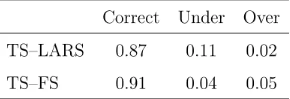
Table 2: Percentage of correctly selected, under- and over-selected lag lengths.
Correct Under Over TS–LARS 0.87 0.11 0.02 TS–FS 0.91 0.04 0.05
selecting a model where some of the relevant predictors are missing in 50% and 61% of all runs, respectively. In this simulation study, over-selection is not an issue. This means that it almost never occurs that redundant predictors are selected, when all relevant ones are already in the model.
We further look at the performance of the TS–LARS and TS–FS procedures with respect to lag length selection. The LARS method is not considered here because it does not perform any lag length selection. There are three possible scenarios: under-, over- or correct selection of the lag length. The results, again for h = 1, are summarized in Table 2. In a large majority of the simulation runs, both the TS–LARS and the TS–FS algorithms select the correct lag length. In the other cases, the lag length is taken too short rather than too long.
To conclude, we may say that the BIC criterion succeeds reasonably well in specifying the correct model, both in terms of the number of relevant predictors and in terms of the lag length. The fully correctly specified model with p= 1 andk = 5
method. This is substantially higher than for the TS–FS method, which has a hit rate of only 8%. When interpreting these rather low numbers, one should take into account that the number of candidate models is very large, and the time series of moderate length T = 150. Moreover, even when the number of relevant predictors is not correctly specified, the resulting model may still have very good forecasting performance, as will be discussed in the remainder of this section.
Forecast performance
We study the out-of-sample forecast performance of the TS–LARS, LARS and TS– FS procedures and make a comparison with the DFM method discussed in Section 3. In every simulation run, we fit the models selected by the different procedures to the simulated data-set of length 150. We then obtain one to five step ahead forecasts for observations 151 to 155. These forecasts are compared to the realized values of the time series as simulated according to the data generating process. The performance of the forecast methods is then compared using the Mean Squared Forecast Error at horizon h: MSFEh = 1 M M X i=1 (yi,150+h−yi,ˆ 150+h)2,
where the index i indicates the simulation runs and M = 2000 is the number of simulation runs.
The results for the first simulation setting are presented in Table 3, where the simulated out-of-sample MSFEh is reported forh= 1, . . . ,5. First of all, we observe
that for all methods the MSFEh steeply increases in h, as is to be expected. Most
striking is that for almost all forecast horizons the TS–LARS method yields the smallest MSFEh. In 14 out of 15 cases, as shown by applying a paired t-test (p
-value reported in the table), the MSFEh of the TS-LARS method is significantly
smaller than for the other methods. At horizon 5 the LARS method performs best, but the difference with TS–LARS is not significant.
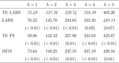
Table 3: Simulated MSFEh at several forecast horizons using the TS–LARS, LARS,
TS–FS and DFM method. Series are generated from a linear time series model. The smallest MSFEs are indicated in italics; p-values of a paired t-test for equal MSFEh
with respect to TS–LARS are given between parentheses.
h= 1 h= 2 h= 3 h= 4 h= 5 TS–LARS 55.49 127.36 220.74 316.30 403.26 LARS 76.55 145.70 234.65 322.20 403.13 (<0.01) (<0.01) (<0.01) (0.03) (0.67) TS–FS 59.08 132.32 227.96 333.03 423.87 (<0.01) (<0.01) (0.01) (<0.01) (<0.01) DFM 73.64 149.25 247.55 337.19 420.34 (<0.01) (<0.01) (0.01) (<0.01) (0.01)
that it is worth taking lagged values of the series into account. More interesting is that TS-LARS outperforms both the more simple TS–FS method, and the popular DFM approach. The worse performance of the DFM method could be explained by the fact that all predictors enter in the construction of the factors, even the redundant ones. Of course, the latter will receive a small weight in the construction of the factor, but they still increase variability of the estimates, leading to poorer forecasting performance.
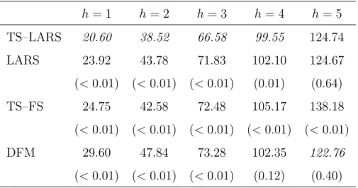
The second simulation scheme is a latent factor model, where one expects the DFM approach to yield better results. However, as can be seen from Table 4, the results are similar to those obtained before. For almost all forecast horizons, the TS–LARS method yields the smallest MSFEh, and the differences with the other
methods are significant in most cases. An exception is h = 5, where the DFM method is better, but the difference with TS–LARS is not significant. It is, however, worth mentioning that for h= 5 the DFM approach mostly selectsk= 0 predictors,
Table 4: Simulated MSFEh at several forecast horizons using the TS–LARS, LARS,
TS–FS and DFM method. Series are generated from a latent factor model. The smallest MSFEs are indicated in italics; p-values of a paired t-test for equal MSFEh
with respect to TS–LARS are given between parentheses.
h= 1 h= 2 h= 3 h= 4 h= 5 TS–LARS 20.60 38.52 66.58 99.55 124.74 LARS 23.92 43.78 71.83 102.10 124.67 (<0.01) (<0.01) (<0.01) (0.01) (0.64) TS–FS 24.75 42.58 72.48 105.17 138.18 (<0.01) (<0.01) (<0.01) (<0.01) (<0.01) DFM 29.60 47.84 73.28 102.35 122.76 (<0.01) (<0.01) (<0.01) (0.12) (0.40)
selection of predictors, i.e. LARS and TS–FS, also generally yield better results than forecasting using diffusion indices.
We conclude that for the simulation schemes under consideration, the TS–LARS method outperforms its competitors, in particular for short term forecasting.
5
APPLICATIONS
5.1
Predicting Aggregate Industrial Production Growth in
the US Using Many Economic Indicators.
To illustrate the performance of the TS–LARS method using real data, we repeat the example elaborated by Stock and Watson (2002a) and Stock and Watson (2002b) for forecasting US industrial production growth. The data used are available on Mark W. Watson’s homepage1and were previously used in, for instance, Stock and Watson
(2005) and de Poorter et al. (2007). The data set includes 132 time series covering many different aspects of the US economy, such as price indices, unemployment rates, interest rates and money supply numbers. There is no missingness in the data and we have 528 monthly observations at our disposal, ranging from January 1960 to December 2003. The aim is to obtain accurate predictions of the industrial production growth rate, while the remaining 131 time series are candidates to be included in the forecast model. The industrial production growth rate is obtained as the log-differences of real US industrial production. A precise description of all 132 series can be found in Stock and Watson (2005). They also describe how the original series can be transformed to be stationary. For some series, this requires differencing, for others taking a log-transformation or log-differencing. We apply the same transformations.
Using the TS–LARS algorithm, we obtain a ranking of the predictors according to their additional predictive power for one-month-ahead US industrial production growth. The top-5 ranking, as obtained by the TS–LARS method, is presented in Table 5. The highest ranked predictor, the NAPM new orders index, is a survey-based indicator constructed by the National Association of Purchasing Management. More than 300 purchasing and supply executives from across the US indicate recent evolutions in their business with respect to orders, prices and unemployment among other things. The TS–LARS algorithm suggests that the number of new orders is the most important predictor for future growth in industrial production. Other important predictors quantify the number of job openings in newspapers, interest rates, wages and consumer expectations. The smallest BIC value is obtained by including the 4 highest ranked predictors up to one lag in the forecasting model.
To compare the forecast performance of the different methods, we divide the data in an in-sample and an out-of-sample part. The in-sample part of the data ranges from January 1960 to December 1981, with a length of R = T /2. The selected model is recursively estimated for t = R, . . . , T −h, to obtain a series of
Table 5: Top-5 ranking of predictor series for predicting one step ahead US industrial production growth, as obtained by the TS–LARS algorithm.
Ranking Predictor
1 NAPM new orders index
2 Index of help-wanted advertising in newspapers 3 3-month FF spread
4 Average hourly earnings: construction 5 Michigan index of consumer expectations
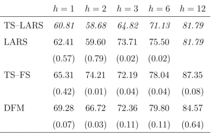
Table 6: Out-of-sample MSFEh(×10000) obtained by the TS–LARS, LARS, TS–FS
and DFM methods, for different forecast horizons. The smallest MSFEh value is in
italics; p-values of the Diebold-Mariano test for equal forecast accuracy compared to TS–LARS are between parentheses.
h= 1 h= 2 h= 3 h= 6 h= 12 TS–LARS 60.81 58.68 64.82 71.13 81.79 LARS 62.41 59.60 73.71 75.50 81.79 (0.57) (0.79) (0.02) (0.02) TS–FS 65.31 74.21 72.19 78.04 87.35 (0.42) (0.01) (0.04) (0.04) (0.08) DFM 69.28 66.72 72.36 79.80 84.57 (0.07) (0.03) (0.11) (0.11) (0.64)
lag length are obtained as discussed in Section 2.2. The mean squared forecast error at horizon h is computed as MSFEh = 1 T −h−R+ 1 T−h X t=R (yt+h−ytˆ+h)2.
The MSFEh is presented in Table 6 for the procedures TS–LARS, LARS, TS–FS
and DFM, at several forecast horizons h. First of all, it is clear that the prediction model selected by the TS–LARS method results in the smallest MSFEhat every
hori-zon. To check whether the observed differences in MSFEh are significant, p-values
are reported for a Diebold-Mariano test for equal out-of-sample predictive accuracy in comparison with the TS–LARS (Diebold and Mariano (1995)). The significance results vary according to the forecast horizon. For short-term forecasts (h= 1 and
h = 2), there is no significant difference between the three methods that rely on variable selection method, LARS, TS–LARS and TS–FS. However, TS–LARS does significantly better than DFM. For 6-month forecasts, the TS–LARS approach gives significantly lower MSFEh than both other variable selection procedures. In
par-ticular, the difference between TS–LARS and LARS is pronounced, showing that accounting for dynamic relationships, as done by the TS–LARS, is worthwhile. At long forecast horizons (h = 12), all methods perform comparably. Note that the TS–LARS selects a model here with only current values of the selected predictors, and therefore yields an identical MSFEh as standard LARS.
The good performance of the TS–LARS method on this well-known data set is striking and promising. The number of retained predicting time series for TS–LARS ranges fromk = 4, for forecast horizon one, tok= 2, for forecast horizon 12, yielding very parsimonious models. Finally, including a total of 12 factors in the forecast model, as was done in Stock and Watson (2002b), does not improve the MSFEh for
5.2
Predicting Country Specific Industrial Production
Us-ing Sentiment Indicators.
As a second application, we study the predictive content of European consumer and production sentiment surveys. We are interested in forecasting Belgian indus-trial production growth and use sentiment surveys from all over Europe. For every EU15 country, we use 5 sentiment indicators: consumer, industrial, retail, services and construction sentiment indicators, resulting in a total of 75 sentiment indica-tors. All these indicators are potential predictors for Belgian industrial production growth. The data range from April 1995 to October 2007, resulting in a total of 151 observations. All the data are publicly available on the Eurostat website2.
Running the TS–LARS algorithm with forecast horizon one leads to the top-5 ranking as presented in Table 7. Using the BIC, one retains the first two predictors, each with one lag. The industrial confidence indicators in France and Belgium are identified as the most powerful predictors for short term forecasting of Belgian indus-trial production growth. This suggests that, in the short run, indusindus-trial production growth might be strongly driven by confidence of the industrial sector itself. Other high ranked predictors, not included in the selected model, are consumer confidence in the Netherlands and retail confidence in Germany and France. It is interesting to note that the five highest ranked predictors are from Belgium itself or neighboring countries. For one-year-ahead forecasting (h= 12) of Belgian industrial production growth, the TS–LARS method selects the Belgian and German consumer confidence indicators to be included in the prediction model. So, in the long run, industrial production growth is more accurately predicted by consumer confidence than by confidence in the industrial sector.
To compare the forecast performance of the TS–LARS method to the LARS, TS– FS and DFM, we compare out-of-sample forecasts. The in-sample range includes the first 75 observations and we proceed in the same way as in Section 5.1. The results of
Table 7: Top-5 ranking of predictor series for predicting one step ahead Belgian industrial production growth, as obtained by the TS–LARS algorithm.
Ranking Predictor
1 Industrial Confidence, France 2 Industrial Confidence, Belgium
3 Consumer Confidence, the Netherlands 4 Retail Confidence, Germany
5 Retail Confidence, France
the out-of-sample forecast comparisons are presented in Table 8, where the MSFEh
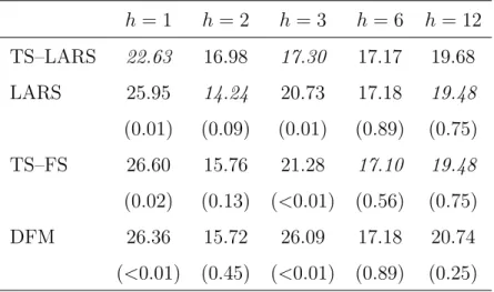
is reported for the TS–LARS, LARS, TS–FS and DFM methods and for several forecast horizons. For forecasting one-month-ahead industrial production growth, the TS–LARS gives the best results. Even more, the TS–LARS is significantly better than all three other methods. No significant differences are obtained for two-months-ahead forecasts, but for three-two-months-ahead we again see that the TS–LARS performs significantly better than the other three considered methods. For longer forecast horizons, all methods perform comparably.
6
CONCLUSION
The LARS procedure, as presented in Efron et al. (2004), is a fast and well-performing method for model selection with cross-sectional data. We propose a new version of the LARS especially designed for time series data and call it the TS–LARS. The new procedure takes the dynamics of the time series into account by selecting blocks of variables. Each block consists of a number of lagged series of a predictor. The good performance of the TS–LARS method is demonstrated by means of a simulation study. It performs better than the standard LARS method,
Table 8: Out-of-sample MSFEh (×1000) obtained by the TS–LARS, LARS, TS–FS
and DFM methods, for different forecast horizons. The smallest MSFEh value is in
italics; p-values of the Diebold-Mariano test for equal forecast accuracy compared to TS–LARS are between parentheses.
h= 1 h= 2 h = 3 h= 6 h= 12 TS–LARS 22.63 16.98 17.30 17.17 19.68 LARS 25.95 14.24 20.73 17.18 19.48 (0.01) (0.09) (0.01) (0.89) (0.75) TS–FS 26.60 15.76 21.28 17.10 19.48 (0.02) (0.13) (<0.01) (0.56) (0.75) DFM 26.36 15.72 26.09 17.18 20.74 (<0.01) (0.45) (<0.01) (0.89) (0.25)
performance, the TS–LARS method shows better results than the dynamic factor model.
In the first empirical application, we apply the TS–LARS method to a large data set to identify which predictors are most informative for future US monthly industrial production growth rates. The highest ranked short-term predictor is the “NAPM new orders index” indicating that evolutions in the number of placed orders is a good predictor for industrial production growth. The second application studies the predictive content of EU business and consumer surveys for future Belgian monthly industrial production growth rates. The TS–LARS procedure indicates that the industrial confidence indicators of both France and Belgium are the most informative short-term predictors. The models selected by the TS–LARS procedure shows good forecast performance as compared to a dynamic factor model, especially for short term forecasting.
In this article, the TS–LARS method acted as a variable selection technique, after which a standard OLS-fit was applied to the selected model. Our experience is
that the selected model typically contains only few predictors, avoiding overfitting by OLS of the selected model. In the examples considered in this paper, parsimonious prediction models were obtained by making use of an OLS fit. In cases where the TS–LARS method would yield a fairly large prediction model, estimation by OLS can be improved upon, since it is well known that OLS estimators may have high variance in models with too many predictors. A solution would be to use a penalized version of OLS, for example the LASSO estimators (Tibshirani (1996)), instead. Alternatively, one could use TS–LARS both as a variable selection and as a model fitting procedure, using the shrinked OLS regression estimates computed in the TS–LARS algorithm outlined in Section 2.1.
A distinct feature of TS–LARS is that it allows for a ranking of the different predictors. This ranking differs according to the series one wants to predict and the forecast horizon. The highest ranked time series are the ones that need to be followed up closely by the forecaster. If data monitoring is expensive or time-consuming, then one might continue to track only the highly ranked series, and not the less informative ones. To conclude, we think that the use of TS–LARS algorithm for predicting time series using many predictors yields parsimonious and easy-to-interpret models, with good forecasting performance. While the good properties of the LARS algorithm have been well documented for cross-sectional data, this paper present its extension to the time series setting. The obtained results are very promising and might generate a new stream of research on forecasting with high dimensional time series.
Acknowledgements: This research was supported by the K.U.Leuven Research Fund and the Fonds voor Wetenschappelijk Onderzoek (Contract number G.0594.05).
Appendix
Proof of equation (5). The left hand side of equation (4) can be rewritten as
R2(z0−γzˆ0 ∼x(1)) = 1− (z0−γzˆ0)0(I−H(1))(z0−γzˆ0) (z0−γzˆ0)0(z0−γzˆ0) . with (z0−γzˆ0)0(I−H(1))(z0−γzˆ0) = (z0−γH(1)z0)0(I−H(1))(z0−γH(1)z0) = z0 0(I −γH(1))(I−H(1))(I−γH(1))z0 = z0 0(I −H(1))z0, (A.14) where we used the well known properties H0
(1) = H(1) and H(1)H(1) = H(1) of the projection matrix. Note that the value of (A.14) does not depend on γ anymore. The right hand side of equation (4) equals
R2(z0−γzˆ0 ∼xj) = 1− (z0−γzˆ0)0(I −Hj)(z0−γzˆ0) (z0−γzˆ0)0(z0−γzˆ0) , with (z0−γzˆ0)0(I−Hj)(z0−γzˆ0) = (z0−γH(1)z0)0(I−Hj)(z0−γH(1)z0) (A.15) = z0 0[(I−γH(1))(I−Hj)](I−γH(1))z0 = z0 0 I−Hj + (H(1)Hj +HjH(1)−2H(1))γ +(H(1)−H(1)HjH(1))γ2 z0. (A.16)
So equation (4) holds if and only if (A.14) and (A.16) are equal to each other. This results in the following quadratic equation (5) for γ.
Finally, note that (5) will always have a root between zero and one, and this for everyj not in the active set. Indeed, forγ = 0 we haveR2(z
0 ∼x(1))≥R2(z0 ∼xj),
by definition of the first index in the active set. On the other hand, for γ = 1 we have 0 =R2(z
0−zˆ0 ∼x(1))≤R2(z0−zˆ0 ∼xj). Hence, there must exist aγ between
Proof of equation (6). Recall that ˆz0 = H(1)z0 and ˜x(1) = ˆz0/s1. The following relations hold: z0 0H(1)z0 =z00H(1)H(1)z0 = ˆz00zˆ0 = (T −1)s21 (A.17) z0 0(H(1)Hj +HjH(1)−2H(1))z0 = ˆz00Hjz0+z00Hjzˆ0−2ˆz00H(1)zˆ00 = 2(s1x˜0(1)Hjz0−zˆ00zˆ00) = 2s1(˜x0(1)Hjz0−(T −1)s1) (A.18) z0 0(H(1)−H(1)HjH(1))z0 = ˆz00zˆ0−zˆ00Hjzˆ0 = s21((T −1)−x˜0 (1)Hjx˜(1)) (A.19) Inserting relations (A.17), (A.18) and (A.19) in (5) results in (6).
Proof of Lemma 1. The three statements of the lemma will be proven by induction. For k= 1, we know that
r1 = Cor(z0,x˜(1)) = Cor(z0,zˆ0)≥0,
so (a) holds for k = 1. Since the index (1) by construction yields the largest
R2(z
0 ∼ xj), (b) holds for k = 1. For proving (c) for k = 1, note that we already
showed that (5) always has a solution between zero and one. Every solution of (5) multiplied by s1 then solves (6) for k = 1, since
R2(z0−γzˆ0 ∼x(1)) =R2(z0−γs1x˜(1) ∼x(1)) = R2(z0−γs1x˜(1) ∼x˜(1)). From a1 = 1, since ˜x(1) is the equiangular vector in the first step, and from r1 =s1, since z0 has unit variance, it follows that (c) holds fork = 1.
Suppose now that the three statements of Lemma 1 hold for k−1. Now we will prove that they also hold for step k. First of all, we have for every i in 1, . . . , k−1
Cor(zk−1,x˜(i)) = Cov(zk−1,x˜(i))
which does not depend on i. Here, we used (a) for k−1, and (7). The inequality holds since (c) is assumed to hold for k−1. Furthermore, since condition (9) holds in step k−1, it follows that
R2(zk−1 ∼x˜(k−1)) =R2(zk−1 ∼x(k)) or Cor2(zk−1 ∼x˜(k−1)) = Cor2(zk−1 ∼x˜(k)). Since ˜x(k) is proportional to the fitted values in the OLS regression of zk−1 on x(k), one also has Cor(zk−1,x˜(k−1)) = Cor(zk−1,x˜(k))≥0. We conclude that (a) holds for step k.
To prove (b), suppose that there exists a j not belonging to the active set in step k
such that
rk2 =R2(zk−1 ∼x˜(k))< R2(zk−1 ∼xj). (A.21)
We use the shortened notationsf0(γ) = R2(zk−2−γuk−1 ∼x˜(k−1)), for the left hand side of condition (9) at step k−1, and fj(γ) =R2(zk
−2−γuk−1 ∼xj), for the right
hand side of condition (9) at step k−1. By definition, γk−1 is the first crossing of the two curves f(k)(γ) andf0(γ), for γ >0. Since (b) is assumed to be hold at step
k−1, we have f0(0)≥fj(0). But definition (8) and (A.21) imply that
f0(γk−1) =f(k−1)(γk)< fj(γk−1).
Hence, there must exist a crossing off0(γ) andfj(γ) at a ˜γstrictly smaller thanγk−1. This contradicts the definition of γk−1, so (A.21) can not hold, proving statement (b).
Finally, let us show that (c) holds at step k. It is sufficient to show that there always exists a solution of equation (9) in the interval [0, rk/ak]. Now note that for
γ = 0, the left hand side of (9) is larger than the right hand side, since we have already proven (b) for step k. On the other hand, for γ =rk/ak, the left hand side of equation (9) equals 0 (as can be seen from equation (A.20)), which is of course smaller than the right hand side of equation (9). Hence, there exists a positive solution, smaller than rk/ak to condition (9).
Proof of equation (11). The left hand side of equation (9) can be rewritten as
R2(zk−1−γuk∼x˜(k)) = Cor2(zk−1 −γuk,x˜(k))
= (Cov(zk−1,x˜(k))−γCov(uk,xk˜ )) 2 Var(zk−1−γuk) = (rk−γak) 2 Var(zk−1−γuk) .
We used here equation (7) and the fact that ˜x(k) has been standardized. The right hand side of condition (9) can be written as
R2(zk−1−γuk ∼xj) = 1− (zk−1−γuk)0(I −Hj)(zk−1−γuk) (zk−1−γuk)0(zk−1−γuk) = (zk−1−γuk)0Hj(zk−1−γuk) (zk−1−γuk)0(zk−1−γuk) ,
where j does not belong to the active set. So condition (9) is equivalent to (rk−γak)2 1 T−1(zk−1 −γuk)0(zk−1−γuk) = (zk−1−γuk) 0Hj(zk −1−γuk) (zk−1−γuk)0(zk−1−γuk)
⇔(T −1)(rk−γak)2 = (zk−1−γuk)0Hj(zk−1−γuk)
⇔(T −1)(r2k−2akrkγ+a2kγ2) = z0
k−1Hjzk−1−2zk0−1Hjukγ+u 0
kHjukγ
2.
After rearranging the terms, equation (11) follows.
References
Bai, J. and Ng, S. (2002), “Determining the Number of Factors in Approximate Factor Models,” Econometrica, 70, 191–221.
— (2007), “Determining the Number of Primitive Shocks in Factor Models,”Journal of Business and Economic Statistics, 25, 52–60.
Bovelstad, H.; Nygard, S.; Storvold, H.; Aldrin, M.; Borgan, O.; Frigessi, A. and Lingjaerde, O. (2007), “Predicting Survival from Microarray Data, a Comparative Study,”Bioinformatics, 23, 2080–2087.
Breiman, L. (1995), “Better subset regression using the nonnegative garrote,” Tech-nometrics, 37, 373–384.
Dante, A. and Watson, M. (2007), “Consistent Estimation of the Number of Dy-namic Factors in a Large N and T Panel,” Journal of Business and Economic Statistics, 25, 91–96.
de Poorter, M.; Ravazzolo, F. and van Dijk, D. (2007), “Predicting the Term Sturcture of Interest Rates,” Working Paper.
Diebold, F. and Mariano, R. (1995), “Comparing predictive accuracy,” Journal of Business and Economic Statistics, 13, 253–263.
Dielman, T. (2001), Applied Regression Analysis, Duxbury Thomson Learning.
Efron, B.; Hastie, T.; Johnstone, I. and Tishirani, R. (2004), “Least Angle Regres-sion,” The Annals of Statistics, 32, 407–451.
Ekkund, J. and Karlsson, S. (2007), “Forecast combination and model averaging using predictive measures,” Econometric Review, 26, 329–363.
Forni, M.; Lippi, M. and Reichlin, L. (2005), “The Generalized Dynamic Factor Model: One-Sided Estimation and Forecasting,” Journal of the American Statis-tical Association, 100, 830–840.
Heij, C.; Groenen, P. and van Dijk, D. (2007), “Forecast comparison of principal component regression and principal covariate regression,” Computational Statis-tics and Data Analysis, 51, 3612–3625.
Hendry, D. and Krozlig, H. (2001),Automatic Econometric Model Selection, London: Timberlake Consultants Press.
Hoover, K. and Krolzig, H. (1999), “Data Mining Reconsidered: Encompassing and the General-to-specific Approach to Specification Search,”Econometrics Journal, 2, 167–191.
Keerthi, S. and Shevade, S. (2007), “A fast tracking algorithm for generalized LARS/LASSO,” IEEE Transactions on Neural Networks, 18, 1826–1830.
Khan, J.; Van Aelst, S. and Zamar, R. (2007), “Robust Linear Model Selection Based on Least Angle Regression,”Journal of the American Statistical Association, 102, 1289–1299.
McCann, L. and Welsch, R. (2007), “Robust variable selection using least angele re-gression and elemental set sampling,”Computational Statistics and Data Analysis, 52, 1289–1299.
Meier, L.; van de Geer, S. and Buhlmann, P. (2008), “The Group LASSO for Logistic Regression,” Journal of the Royal Statistical Society, Series B, 70, 53–71.
Qian, G. and Zhao, X. (2007), “On time series model selection involving many candidate ARMA models,”Computational Statistics and Data Analysis, 51, 6180– 6196.
Saigo, H.; Uno, T. and Tsuda, K. (2007), “Mining Complex Genotypic Features for Predicting HIV-1 Drug Resistance,”Bioinformatics, 23, 2455–2462.
Simila, T. and Tikka, J. (2007), “Input selection and shrinkage in multiresponse linear regression,”Computational Statistics and Data Analysis, 52, 406–422.
Stock, J. and Watson, M. (2002a), “Forecasting Using Principal Components From a Large Number of Predictors,” Journal of the American Statistical Association, 97, 1167–1179.
— (2002b), “Macroeconomic Forecasting Using Diffusion Indexes,” Journal of Busi-ness and Economics Statistics, 20, 147–162.
— (2006), “Forecasting with many predictors,” Handbook of Economic Forecasting, Elliott, G., Grange, C.W.J., Timmermann, A., 515–554.
Stock, J. and Watson, W. (2005), “Implications of Dynamic Factors for VAR Analy-sis,” Working Paper.
Sulkava, M.; Tikka, J. and Hollmen, J. (2006), “Sparse regression for analyzing the development of foliar nutrient concentrations in coniferous trees,” Ecological Modelling, 191, 118–130.
Tibshirani, R. (1996), “Regression shrinkage and selection via the LASSO,”Journal of the Royal Statistical Society Series B, 58, 267–288.
Yuan, M.; Joseph, V. and Lin, Y. (2007), “An efficient variable selection approach for analyzing designed experiments,” Technometrics, 49, 430–439.
Yuan, M. and Lin, Y. (2006), “Model selection and estimation in regression with grouped variables,” Journal of the Royal Statistical Society Series B, 68, 49–67.