NBER WORKING PAPER SERIES
OPTIMAL MONETARY POLICY Aubhik Khan
Robert G. King Alexander L. Wolman
Working Paper9402
http://www.nber.org/papers/w9402
NATIONAL BUREAU OF ECONOMIC RESEARCH 1050 Massachusetts Avenue
Cambridge, MA 02138 December 2002
The authors thank Bernardino Adao, Orazio Attanasio, Isabel Correia, Bill Dupor, Chris Erceg, Steve Meyer, Pedro Teles, Julia Thomas and Michael Woodford for useful conversations and comments. In addition, we have benefited from presentations at the June 2000 Banco de Portugal Conference on Monetary Economics; the NBER Summer Institute, the Society for Economic Dynamics meeting, the Federal Reserve System Committee, Rutgers University, and the University of Western Ontario. The views expressed here are the authors’ and not necessarily those of the Federal Reserve Banks of Philadelphia or Richmond, the Federal Reserve System or the National Bureau of Economic Research.
© 2002 by Aubhik Khan, Robert G. King, and Alexander L. Wolman. All rights reserved. Short sections of text not to exceed two paragraphs, may be quoted without explicit permission provided that full credit including, © notice, is given to the source.
Optimal Monetary Policy
Aubhik Khan, Robert G. King, and Alexander L. Wolman NBER Working Paper No. 9402
December 2002 JEL No. E5
ABSTRACT
Optimal monetary policy maximizes the welfare of a representative agent, given frictions in the economic environment. Constructing a model with two sets of frictions -- costly price adjustment by imperfectly competitive firms and costly exchange of wealth for goods -- we find optimal monetary policy is governed by two familiar principles. First, the average level of the nominal interest rate should be sufficiently low, as suggested by Milton Friedman, that there should be deflation on average. Yet, the Keynesian frictions imply that the optimal nominal interest rate is positive. Second, as various shocks occur to the real and monetary sectors, the price level should be largely stabilized, as suggested by Irving Fisher, albeit around a deflationary trend path. Since expected inflation is roughly constant through time, the nominal interest rate must therefore vary with the Fisherian determinants of the real interest rate. Although the monetary authority has substantial leverage over real activity in our model economy, it chooses real allocations that closely resemble those which would occur if prices were flexible. In our benchmark model, there is some tendency for the monetary authority to smooth nominal and real interest rates.
Aubhik Khan Robert G. King Alexander L. Wolman
Research Department Department of Economics Research Department Federal Reserve Bank Boston University Federal Reserve Bank of Phildelphia 270 Bay State Road of Richmond
10 Independence Mall Boston, MA 02215 P.O. Box 27622 Philadelphia, PA 19106 and NBER Richmond, VA 23261
1
Introduction
Three distinct intellectual traditions are relevant to the analysis of how optimal mon-etary policy can and should regulate the behavior of the nominal interest rate, output and the price level.
The Fisherian view: Early in this century, Irving Fisher [1923,1911] argued that the business cycle was “largely a dance of the dollar” and called for stabilization of the price level, which he regarded as the central task of the monetary authority. Coupled with his analysis of the determination of the real interest rate [1930] and the nominal interest rate [1896], the Fisherian prescription implied that the nominal interest rate wouldfluctuate with those variations in real activity which occur when the price level is stable.
The Keynesian view: Stressing that the market-generated level of output could be inefficient, Keynes [1936] called for stabilization of real economic activity by fiscal and monetary authorities. Such stabilization policy typically mandated substantial variation in the nominal interest rate when shocks, particularly those to aggregate demand, buffeted the economic system. Prices were viewed as relatively sticky and little importance was attached to the path of the price level.
The Friedman view: Evaluating monetary policy in a long-run context with fully flexible prices, Friedman [1969] found that an application of a standard microeco-nomic principle of policy analysis — that social and private cost should be equated — indicated that the nominal interest rate should be approximately zero. Later authors used the same reasoning to conclude that the nominal interest rate should not vary through time in response to real and nominal disturbances, working within flexible price models of businessfluctuations.1
There are clear tensions between these three traditions if real forces produce ex-pected changes in output growth that affect the real interest rate. If the price level is constant, then the nominal interest rate must mirror the real interest rate, violating Friedman’s rule. If the nominal interest rate is constant, as Friedman’s rule suggests, then there must be expected inflation or deflation to accommodate the movement in the real rate, and thus Fisher’s prescription cannot be maintained. The variation in inflation and nominal interest rates generally implied by Keynesian stabilization conflicts with both the Friedman and Fisherian views.
We construct a model economy that honors each of these intellectual traditions and study the nature of optimal monetary policy. There are Keynesian features to the economy: output is inefficiently low becausefirms have market power andfluctuations reflect the fact that all prices cannot be frictionlessly adjusted. However, as in the New Keynesian research on price stickiness that begins with Taylor [1980],firms are forward-looking in their price setting and this has dramatic implications for the design of optimal monetary policy. In our economy, there are also costs of converting wealth into consumption. These costs can be mitigated by the use of money, so that there are
social benefits to low nominal interest rates as in Friedman’s analysis. The behavior of real and nominal interest rates in our economy is governed by Fisherian principles. Following Ramsey [1927] and Lucas and Stokey [1983], we determine the alloca-tion of resources which maximizes welfare of a representative agent given the resource constraints of the economy and additional constraints that capture the fact that the resource allocation must be implemented in a decentralized private economy. The staggered nature of price-setting in our economy means that there are many imple-mentation constraints that must be respected.2 We assume that there is full
commit-ment on the part of a social planner for the purpose of determining these allocations andfind that two familiar principles govern monetary policy in our economy.
1. The Friedman prescription for deflation. The average level of the nominal interest rate should be sufficiently low that there should be deflation on average, as suggested by Milton Friedman. Yet, the Keynesian frictions generally imply that there should be a positive nominal interest rate.
2. The Fisherian prescription for eliminating price-level surprises. As shocks occur to the real and monetary sectors, the price level should be largely stabilized, as suggested by Irving Fisher, albeit around a deflationary trend path. (In modern language, there is only a small “base drift” for the price level path). Since expected inflation is relatively constant through time, the nominal interest rate must therefore vary with the Fisherian determinants of the real interest rate. However, there is some tendency for nominal and real interest rate smoothing relative to the outcomes in aflexible price economy.
By contrast, wefind less support for Keynesian stabilization policy. Although the monetary authority has substantial leverage over real activity in our model economy, it chooses allocations that closely resemble those which would occur if prices were flexible. When departures from this flexible price benchmark occur under optimal policy, they are not always in the traditional direction: in one example, a mone-tary authority facing a high level of government demand chooses to contract private consumption relative to theflexible price outcome, rather than stimulating it.
The organization of the paper is as follows. In section 2, we outline the main features of our economic model and define a recursive imperfectly competitive equi-librium. In section 3, we describe the nature of the general optimal policy problem that we solve, which involves a number of forward-looking constraints. We outline how to treat this policy problem in an explicitly recursive form. Our analysis thus ex-emplifies a powerful recursive methodology for analyzing optimal monetary policy in richer models that could include capital formation, state dependent pricing and other frictions such as efficiency wages or search. In section 4, we identify four distortions 2Ireland [1996], Goodfriend and King [2001] and Adao, Correia and Teles [2001] use a similar
approach to study models with pre-set prices. These models contain only one or two implementation constraints.
present in our economic model, which are summary statistics for how its behavior can differ from a fully competitive, nonmonetary business cycle model. In section 5, we discuss calibration of a quantitative version of our model, including estimation of a money demand function.
In section 6, we discuss the results which lead to the first principle for monetary policy: the nominal interest rate should be set at an average level that implies de-flation, but it should be positive. We show how this steady-state rate of deflation depends on various structural features of the economy including the costs of transact-ing with credit, which give rise to money demand, and the degree of price-stickiness.3
In our benchmark calibration, which is based on an estimated money demand function using post-1958 observations, the extent of this deflation is relatively small, about .75%. It is larger (about 2.3%) if we use estimates of money demand based also on observations from 1948-1958; this longer sample includes intervals when interest rates and velocity were both low, which Lucas [2000] argues are important for estimation of the demand for money and the calculation of associated welfare cost measures. In addition, a smaller degree of market power or less price stickiness make for a larger deflation under optimal policy.
In section 7, we describe the near-steady state dynamics of the model under optimal policy. Looking across a battery of specifications, wefind that these dynamics display only minuscule variation in the price level. Thus, we document that there is a robustness to the Fisherian conclusion in King and Wolman [1999], which is that the price level should not vary greatly in response to a range of shocks under optimal policy. In fact, the greatest price level variation that wefind involves less than a0.5% change in the price level over twenty quarters, in response to a productivity shock which brings about a temporary but large deviation of output from trend, in the sense that the cumulative output deviation is more than 10% over the twenty quarters. Across a range of experiments, output under optimal policy closely resembles output which would occur if all prices wereflexible and monetary distortions were absent. We refer to the flexible price, nonmonetary model as our underlying real business cycle framework. Although the deviations of quantities under optimal policy from their real business cycle counterparts are small, because these deviations are temporary, they give rise to larger departures of real interest rates from those in the RBC solution. We relate the nature of these departures to the nature of constraints on the monetary authority’s policy problem. Section 8 concludes.
2
The model
The model incorporates elements from two important strands of macroeconomic re-search. First, money is a means of economizing on the use of costly alternative media 3By the steady state, we mean the point to which the economy converges under optimal policy
as in the classic analyses of Baumol [1952] and Tobin [1956].4 Second, firms are im-perfect competitors facing infrequent opportunities for price adjustment as in much recent New Keynesian research beginning with Taylor [1980] and Calvo [1983]. To facilitate the presentation of these mechanisms, we view the private sector as divided into three groups of agents. First, there are households which buyfinal consumption goods and supply factors of production. These households also trade in financial markets for assets, including a credit market, and acquire cash balances which can be exchanged for goods. Second, there are retailers, which sellfinal consumption goods to households and buy intermediate products fromfirms. Retailers can costlessly ad-just prices.5 Third, there are producers, who create the intermediate products that retailers use to producefinal consumption goods. Thesefirms have market power and face only infrequent opportunities to adjust prices.
The two sources of uncertainty are the level of total factor productivity,a, and the level of real government purchases,g, which is assumed to befinanced with lump-sum taxes. These variables depend on an exogenous state variable ς, which evolves over time as a Markov process, with the transition probability denoted Υ(ς,·). That is, if the current state is ς then the probability of the future state being in a given set of states B isΥ(ς, B) = Pr{ς0 ∈B |ς =ς}. We thus write total factor productivity as a(ς)and real government spending as g(ς).
In this section, we describe a recursive equilibrium, with households and firms solving dynamic optimization problems given a fixed, but potentially complicated, rule for monetary policy that allows it to respond to all of the relevant state variables of the economy, which are of three forms. Ignoring initially the behavior of the monetary authority, the model identifies two sets of state variables. First, there are the exogenous state variables just discussed. Second, since some prices are sticky, predetermined prices are part of the relevant history of the economy. These variables, s, evolve through time according to a multivalent function Γ where s0 = Γ(s, p
0,π),
with p0 and π being endogenous variables further described below. We allow the
monetary authority to respond to ς and s, but also to a third set of state variables
φ, which evolves according to φ0 = Φ(ς, s,φ). In a recursive equilibrium, p0 and π are functions of the monetary rule, so that the states s evolve according to s0 = Γ(s, p0(ς, s,φ),π(ς, s,φ)) ;we will sometimes write this ass0 =Γ(s,φ,ς). Hence, there
is a vector of state variables σ = (s,φ,ς) that is relevant for agents, resulting from the stochastic nature of productivity and government spending; from the endogenous dynamics due to sticky prices; and, potentially, from the dynamic nature of the monetary rule.
4More specifically, money economizes on credit costs as in Prescott [1987], Dotsey and Ireland
[1996] and Lacker and Schreft [1996].
2.1
Households
Households have preferences for consumption and leisure, represented by the time-separable expected utility function,
Et
∞
j=0
βju(ct+j, lt+j) (1)
The period utility functionu(c, l) is assumed to be increasing in consumptionct and
leisurelt, strictly concave and differentiable as needed. Households divide their time
allocation — which we normalize to one unit — into leisure, market work nt, and
transactions time ht so thatnt+lt+ht=1.
Accumulation of wealth: Households begin each period with a portfolio of claims on the intermediate product firms, holding a previously determined share θt of the
per capita value of these firms.6 This portfolio generates current nominal dividends of θtZt and has nominal market value θtVt, whereVt is measured on a pre-dividend
basis for reasons that will be discussed further below.7 They also begin each period
with a stock of nominal bonds left over from last period which have matured and have market value Bt. Finally, they begin each period with nominal debt arising
from consumption purchases last period, in the amountDt. So, their nominal wealth
is θtVt + Bt − Dt − Tt, where Tt is the amount of a lump sum tax paid to the
government. With this nominal wealth and current nominal wage incomeWtnt, they
may purchase money Mt, buy current period bonds in amount Bt+1, or buy more
claims on the intermediate product firms, each unit of which costs them (Vt−Zt).
Thus, they face the constraint
Mt+
1 1+Rt
Bt+1+θt+1(Vt−Zt)≥θtVt+Bt−Dt−Tt+Wtnt.
We convert this nominal budget constraint into a real one, using a numeraire Pt. At
present this is simply an abstract measure of nominal purchasing power but we are more specific later about its economic interpretation. Denoting the rate of inflation between period t−1and periodt asπt= PPtt
−1−1, the realflow budget constraint is
mt+ 1 1+Rt bt+1+θt+1(vt−zt)≤θtvt+ bt 1+πt − dt 1+πt − τt+wtnt,
6Since this is a representative agent model, there are many equivalent ways of setting up the
financial markets in which households can trade. One possibility would be to specify that households can trade Arrow-Debreu securities which pay off a real unit in a single state of the world. If the probability-normalized real price of such a security on future state σ0 is ρ(σ,σ0) in state σ,
then a household would value the cash flows of the ith firm according to the recursion v(i,σ) =
z(i,σ) +E{ρ(σ,σ0)v(i,σ0)}. It would therefore be possible, as Michael Woodford has stressed to us,
to derive rather than impose thefirm valuation equations that we use in this paper.
7Z
tandVtare aggregates of the dividends and values of individual firms in a sense that we will
with lower case letters representing real quantities when this does not produce nota-tional confusion (real lump sum taxes are τt = PTtt).8
Money and transactions: Although households have been described as purchasing a single aggregate consumption good, we now reinterpret this as involving many individual products — technically, a continuum of products on the unit interval — as in many studies following Lucas [1980]. Each of these products is purchased from a separate retail outlet at a price Pt. Each customer buys a fraction ξt of goods with
credit and the remainder with cash. Hence, the households’ demand for nominal money satisfies Mt = (1−ξt)Ptct. Nominal debt is correspondingly Dt+1 = ξtPtct,
which must be paid next period. Following our convention of using lower case letters to define real quantities, define pt ≡ Pt
Pt. The real money demand of the household
takes the formmt= (1−ξt)ptct and similarly dt+1 =ξtptct.
We think of each final consumption good purchase having a random fixed time cost, which must be borne if credit is used. This cost is known after the customer has decided to purchase a specific amount of the product, but before the customer has decided whether to use money or credit to finance the purchase. Let F (·) be the cumulative distribution function for time costs. If credit is used for a particular good, then there are time costs ν and the largest time cost is given by ¯νt=F−1(ξt).
Thus, total time costs areht=
F−1(ξ
t)
0 νdF(ν).The household uses credit when its
time cost is below the critical level given byF−1(ξ
t) and uses money when the cost
is higher.
2.1.1 Maximization Problem
Although the household’s individual state vector can be written as its holdings of each asset (θ, b, d), it is convenient here — as in many other models — to aggregate these assets into a measure of wealth$=vθ+1+b−dπ−τ. We letU be the value function, the indirect lifetime utility function of a household. The recursive maximization problem is then
8For example m
t = MPtt and vt, zt and wt are similarly defined. The two exceptions are the
U($;σ) = max ξ,c,l,n,m,θ0,b0,d0{u(c, l) +βEU($ 0;σ0)|σ} (2) subject to m+ 1 1+Rb 0+θ0(v−z)≤$+wn (3) n=1−l−h (4) h= F−1(ξ) 0 ν dF(ν) (5) m = (1−ξ)pc (6) d0 =ξpc (7)
The right-hand side of (3) is financial wealth plus labor income ($+wn); the left-hand side is purchases of money, discount bonds, and shares (the net cost of stock is its ex-dividend price). The household is assumed to vieww, v, R, z, p,π andτ =T /P as functions of the state vector,σ. The conditional expectationβEU($0;ς0, s0,φ0)|σ} is equal to U($0;ς0, s0,φ0)Υ(ς,dς0)}, taking as given the laws of motion s0 = Γ(σ) and φ0 = Φ(σ) discussed above and the definition $0 = v0θ0 + b0−d0
1+π0 −τ0. We will
return to the discussion of the determinants and consequences of inflation later. 2.1.2 Efficiency conditions
We consolidate the household’s constraints (3) - (7) into a single constraint, by elim-inating hours worked, as is conventional. We also substitute out for money, using m= (1−ξ)pc,and future debt, usingd0 =ξpc to simplify this constraint further. Let
λ, which has the economic interpretation as the shadow value of wealth, represent the multiplier for this combined constraint. Then, we use the envelope theorem to derive D1U($,;σ) =λ.9 We can then state the household’s efficiency conditions as
c : D1u(c, l) =λ(1−ξ)p+βE[λ0 p 1+π0ξ]|σ (8) ξ : λpc=λwF−1(ξ) +βE[λ0 p 1+π0c]|σ (9) l : D2u(c, l) =wλ (10) b0 : 1 1+Rλ=βE[λ 0 1 1+π0]|σ (11) θ0 : (v−z)λ=βE[λ0v0]|σ (12)
9We use “envelope theorem” as short-hand for analyses following Benveniste and Scheinkman
as well as (3)-(7). Condition (8) states that the marginal utility of consumption must be equated to the full cost of consuming, which is a weighted average of the costs of purchasing goods with currency and credit. Condition (9) equates the marginal benefit of raisingξto its net marginal cost, the latter being the sum of the current time cost and the future repayment cost. Condition (10) is the conventional requirement that the marginal utility of leisure is equated to the real wage rate times the shadow value of wealth. The last two conditions specify that holdings of stocks and bonds are efficient.
2.2
Retailers
Retailers create units of the final good according to a constant elasticity of substitu-tion aggregator of a continuum of intermediate products, indexed on the unit interval, i∈[0,1].10 Retailers createq units offinal consumption according to
q = q(i)ε−ε1di
ε ε−1
, (13)
whereεis a parameter. In our economy, however, there will be groups of intermediate goods-producing firms which will all charge the same price for their good within a period and they can be aggregated easily. Let the j-th group have fraction ωj and
charge a nominal price Pj. Then the retailer allocates its demands for intermediates
across the J categories, solving the following problem: min qj (1+R) J−1 j=0 ωjpjqj (14) subject to q = ( J−1 j=0 ωjqj ε−1 ε ) ε ε−1, (15) where pj = Pj
P is the relative price of the j-th set of intermediate inputs. Retailers
viewRand{pj}jJ=0−1 as functions ofσ. The nominal interest factor(1+R)affects the
retailer’s expenditures because, as is further explained below, the retailer must borrow tofinance current production. This cost minimization problem leads to intermediate input demands of a constant elasticity form
qj = p−jε q,¯ (16)
whereqis the retailer’s supply of the composite good. Cost minimization also implies a nominal unit cost of production — an intermediate goods price level of sorts — given 10Note that this continuum of intermediate goodsfirms is distinct from the continuum of retail
by P = [ J−1 j=0 ωjP (1−ε) j ] 1 1−ε. (17)
This is the price index which we use as numeraire in the analysis above. As the retail sector is competitive and all goods are produced according to the same technology, it follows that thefinal goods price must satisfyP = (1+R(σ))P and that the relative price of consumption goods is given by
p(σ) =1+R(σ). (18)
Since they have no market power or specialized factors, retailers earn no profits. Hence, their market value is zero and does not enter in the household budget con-straint. At the same time, they are borrowers, making their expenditures at t and receiving their revenues at t+1. That is: for each unit of sales, the retailfirm receives revenues in money or credit. Each of these are cashflows which are effectively in date t+1 dollars. If thefirm receives money, then it must hold it “overnight.” If the firm takes credit, then it is paid only at date t+1 with no explicit interest charges, as is the practice with credit cards in many countries.
2.3
Intermediate goods producers
The producers of intermediate products are assumed to be monopolistic competitors and face irregularly timed opportunities for price adjustment. For this purpose, we use a general stochastic adjustment model due to Levin [1991], as recently exposited in the Dotsey, King and Wolman [1999] analysis of state dependent pricing. In this setup, a firm which has held its pricefixed for j periods will be permitted to adjust with probability αj. With a continuum of firms, the fractions ωj are determined
by the recursions ωj = (1− αj)ωj−1 for j = 1,2, ...J −1 and the condition that ω0 =1− Jj=1−1ωj.
Each intermediate product i on the unit interval is produced according to the production function
y(i) =an(i), (19)
with labor being paid a nominal wage rate ofW and beingflexibly reallocated across sectors. Nominal marginal cost for all firms is accordingly W/a. Let p(i) ≡ PP(i) be thei−th intermediate goods producer’s relative price and w = WP, the real wage, so that real marginal cost is ψ =w/a.
Intermediate goodsfirms face a demand given by
y(i) =p(i)−εq(σ), (20)
with the aggregate demand measure being q(σ) = c(σ) +g(ς), i.e., the sum of household and government demand.
2.3.1 Maximization Problem
Intermediate goodsfirms maximize the present discounted value of their real monopoly profits given the demand structure and the stochastic structure of price adjustment. Using (19) and (20), current profits may be expressed as
z(p(i) ;σ) =p(i)y(i)−w(σ)n(i) =p(i)−εq(σ) p(i)−w(σ)
a(ς) . (21)
All firms that are adjusting at date t will choose the same nominal price, which we call P0, which implies a relative price p0 = PP0. The mechanical dynamics of relative
prices are simple to determine. Given that a nominal price is set at a level Pj, then
the current relative price is pj =Pj/P. If no adjustment occurs in the next period,
then the future relative price satisfies
p0j+1= pj
1+π0. (22)
A price-setting intermediate goods producer solves the following maximization prob-lem: v0(σ) = max p0 [z(p0;σ) +E{β λ(σ0) λ(σ) α1v 0(σ0) + (1−α 1)v1(p01,σ0) }|σ], (23)
with the maximization taking place subject top0 1 = P0 1 P0 = P0 P P P0 = p0/(1+π0). A few
comments about the form of this equation are in order. First, the discount factor used byfirms equals households’ shadow value of wealth in equilibrium, so we impose that requirement here. Second, as is implicit in our profit function, thefirm is constrained by its production function and by its demand curve, which depends on aggregate consumption and government demand. Third, thefirm knows that at datet+1, with probabilityα1it will adjust its price and the current pricing decision will be irrelevant
to its market value (v0). With probability 1
−α1 it will not adjust its price and the
current price will be maintained, resulting in a market valuev1. Our notation is that
the superscriptj invj indicates the value of afirm which is maintaining its pricefixed at the level set at datet−j, i.e., Pj,t =P0,t−j. Thus, we have forj =1, . . . , J−2,
vj(pj,σ) =z(pj;σ) +E{β λ(σ0) λ(σ)[αj+1v 0(σ0) + (1−α j+1)vj+1(pj0+1,σ0)]}|σ, (24) with p0 j+1 = pj
1+π0. Finally, in the last period of price fixity, all firms know that they
will adjust for certain so that
vJ−1(pJ−1,σ) =z(pJ−1;σ) +E{β
λ(σ0)
λ(σ)[v
0
(σ0)]}|σ. (25)
These expressions imply that the aggregate portfolio value and dividends, denoted vt and zt in the household’s problem, are determined as vt =
J−1
zt= J−1
j=0 ωjz(pj,t,σ). Our decision to earlier write the stock market portfolio in
pre-dividend value terms was based on having a ready match with the natural dynamic program for thefirm’s pricing decisions.
2.3.2 Efficiency conditions
In order to satisfy (23), the optimal pricing decision requiresp0 to solve
0 =D1z(p0;σ) +βE λ0 λ(1−α1)D1v 1(p0 1;σ0) 1 1+π0 |σ. (26) From (21), marginal profits are given by
D1z(pj;σ) =q(σ) (1−ε)p−jε+ε
w(σ)
a(σ)p
−ε−1
j . (27)
The optimal pricing condition (26) states that, at the optimum, a small change in price has no effect on the present discounted value. The presence of future inflation reflects the fact that p0
1 = p0/(1+π0), so that when the firm perturbs its relative
price by dp0, it knows that it is also changing its one period ahead relative price by
1/(1+π0) dp0.11 Equations (24) imply D1vj(pj;σ) =D1z(pj;σ) +βE λ0 λ(1−αj+1)D1v j+1(p0 j+1;σ0) 1 1+π0 |σ (28)
for j =1, . . . , J −2, while (25) implies
D1vJ−1(pJ−1;σ) =D1z(pJ−1;σ). (29)
2.4
De
fi
ning the state vector s
We next consider the price component of the aggregate state vector. The natural state is the vector of previously determined nominal prices,[P1,t P2,t... PJ−1,t]. Given these
predetermined nominal prices and the nominal price P0,t set by currently adjusting
firms, the price level Pt is [ Jj=0−1ωjP
(1−ε)
j,t ]
1
1−ε. However, our analysis concerns (i)
households andfirms that are concerned about real objectives as described above; and (ii) a monetary authority who seeks to maximize a real objective as described below. Accordingly, neither is concerned about the absolute level of prices in the initial period
11An individualfirm choosesp
0(i)taking as given the actions of all otherfirms — including other
adjustingfirms — as these affect the price level, aggregate demand and so forth. Specifically,firm i
views the actions of other adjustingfirms asp0(σ), with a law of motion forσdescribed earlier. In
an equilibrium, there is afixed point in that the decision rule of the individual firmp(i,σ)is equal to the functionp0(σ).
of our model (i.e., the time at which the monetary policy rule is implemented). For this reason, we opt to use an alternativereal state vector that captures the influence of predetermined nominal prices, but is compatible with any initial scale of nominal prices.
There are a variety of choices that one might make in defining this real state vector, with the decision based on how completely one seeks to cast the optimal policy problem in terms of real quantities and computational considerations.12,13 In the current analysis, we instead use the simplest and most direct state vector: a vector of lagged relative prices.
The relative prices that will prevail in the economy at date t arep0,t, p1,t, ..., pJ−1,t.
Since nominal prices are sticky (Pj,t=Pj−1,t−1), it follows that
pj,t = Pj,t Pt = Pj−1,t−1 Pt−1 Pt−1 Pt = pj−1,t−1 1+πt , (30)
for j = 1,2, ...J −1. Accordingly, given current inflation, we can account for the
relative prices of sticky prices goods so long as we knowpj,t−1 forj = 0,1,2, ...J −2.
TheseJ−1lagged relative prices thus are chosen to be our real state vector, so that
st−1 = [p0,t−1....pJ−2,t−1].
2.5
Monetary policy
Monetary policy determines the nominal quantity of money. However, just as we normalized lagged nominal prices by the past price level, it is convenient to similarly deflate the money stock. With this normalization, we denote the policy rule by
M(σt), and the nominal money supply is given by
Mt =M(σt)·Pt−1. (31)
Real balances are given by mt =M(σt)·PPt−t1 = M1+(σπtt).14
12For example, King and Wolman [1999] use a state vector that is a vector of lagged real demand
ratios, cj,t−1/cj+1,t−1 for j = 0,1, ...J−3, in order to cast the monetary authority’s problem as
solely involving real quantities.
13Computational considerations might lead one to (i) make the state vectors
t−1= Pj,t/Pt J−2 j=1 wherePt= [1−1ω0 Jh=1−1ωjPj,t(1−ε)] 1 1−ε
is an index of the predetermined part of the price level; and (ii) use related manipulations to eliminate the inflation rate as a current decision variable for the monetary authority. The computational advantage derives from the fact that there are then only
J−2elements of the state vector, whereas there areJ−1elements with the approach presented in the text.
14It is clear from (31) that if the policy rule involves no response to the state, then this generally
does not make the nominal money supply constant, because a constantM()impliesMt=M·Pt−1,
meaning that the path of the money supply is proportional to the past price level. If the monetary authority makes the nominal money supply constant, it must make the past price level part of the state vector, because a constant money supplyM impliesM(σt) =M/Pt−1.
With the general function M(σt) we are not taking a stand on the targets or
instruments of monetary policy. This notation makes clear, however, that the mon-etary authority’s optimal decisions will depend on the same set of state variables as the decisions of the private sector.
2.6
Recursive equilibrium
We now define a recursive equilibrium in a manner that highlights the key elements of the above analysis.15
Definition. For a given monetary policy function M(σ), a Recursive Equilibrium is a set of relative price functions λ(σ),w(σ),{pj(σ)}Jj=0−1, and p(σ); an interest rate
function R(σ); an inflation function π(σ); aggregate production, q(σ); dividends,
z(σ); intermediate goods producers’ profits {zj(σ)}jJ=0−1; value functions U(·) and
{vj(
·)}Jj=0−1; household decision rules ξ(σ), c(σ), l(σ), n(σ), m(σ), θ0(σ), b0(σ), d0(σ) ; intermediate goods producers’ relative quantities, {q
j(σ)}Jj=0−1; intermediate
goods producers’ relative prices, {pj(σ)}Jj=0−1 and a law of motion for the aggregate
state σ = (ς, s,φ), ς0 ∼ Υ(ς,·), s0 = Γ(σ) and φ0 = Φ(σ) such that: (i) households
solve (2) - (7), (ii) retailers solve (14) - (15), (iii) price-setting intermediate goods producers solve (22) - (25), and (iv) markets clear.
While this definition describes the elements of the discussion above that are im-portant to equilibrium, it is useful to note that a positive analysis of this equilibrium can be carried out without determining the value functionsU(·)and{vj(
·)}Jj=0−1, but by simply relying on thefirst-order conditions. We exploit this feature in our analysis of optimal policy.
3
Optimal policy approach
Our analysis of optimal policy is in the tradition of Ramsey [1927] and draws heavily on the modern literature on optimal policy in dynamic economies which follows from Lucas and Stokey [1983]. In this paper, as in King and Wolman [1999], we adapt this approach to an economy which has real and nominal frictions. Here those frictions are monopolistic competition, price stickiness and the costly conversion of wealth into goods, with the cost affected by money holding. The outline of our multi-stage approach is as follows. First, we have already determined the efficiency conditions of households and firms that restrict dynamic equilibria, as well as the various bud-15The household’s real budget constraint (3) is not included in the equations that restrict
equi-librium, as in many other models, since it is implied by market clearing and the government budget constraint. In equilibrium,θ= 1,b−d= 0, and τ=gso that$=v−g. Thus, current inflation,
πt, does not enter into the household’s decisions. Howevever, it does enter into the dynamics of
get and resource constraints. Second, we manipulate these equations to determine a smaller subset of restrictions that govern key variables, in particular eliminating
M(σt) so that it is clear that we are not taking a stand on the monetary instrument.
Third, we maximize expected utility subject to these constraints. Fourth, we find the absolute prices and monetary policy actions which lead these outcomes to be the result of dynamic equilibrium.16
3.1
Organizing the restrictions on dynamic equilibria
We begin by organizing the equations of section 2 so that they are a set of constraints on the policy maker. To aid in this process and in the statement of the optimal monetary policy problem as an infinite horizon dynamic optimization problem in the next subsection, it becomes useful to reintroduce time subscripts throughout this section.
3.1.1 Restrictions implied by technology and relative demand Thefirst constraint is associated with production. Sincent =
J−1 j=0 ωjnj,t, (19) gives atnt= ( J−1 j=0 ωjp−j,tε)(ct+gt). (32)
The second constraint is associated with the aggregation of intermediate goods in (13), 1= [ J−1 j=0 ωjp1j,t−ε] 1 1−ε. (33)
3.1.2 Restrictions implied by state dynamics
With staggered pricing, the dynamics of the states is just given by (30). Defining the state vector st = [p0t .... pJ−2,t], we can write its dynamic equation in the form
discussed above, st=Γ(st−1, p0t,πt)where Γ takes the form
s1t s2,t . . sJ−1,t = 10 0 1+πt ·I 0 0 s1,t−1 s2,t−1 . . sJ−1,t−1 + 1 0 . . 0 p0,t
whereIis an identity matrix withJ−2rows and columns and0is a row vector with J−2 elements
3.1.3 Restrictions implied by household behavior
The household’s decision rules are implicitly restricted by the equations (3) - (7) and (8) - (12). A planner must respect all of these conditions, but it is convenient for us to use some of them to reduce the number of choice variables, while retaining others. In particular, combining (8), (11) and (18), wefind that the household requires that the marginal utility of consumption is equated to a measure of the full price of consumption, which depends on λt as is conventional, but also onRt andξt because
money or credit must be used to obtain consumption:
D1u(ct, lt) =λt[1+Rt(1−ξt)]. (34)
Combining (9), (10), (11) and (18), the efficient choice between money and credit as a means of payment is restricted by
Rtct=wtF−1(ξt) =
D2u(ct, lt)
λt
F−1(ξt), (35)
which indicates how credit use is related to market prices and quantities. Since
ξ=1−P cM, this restriction implicitly defines the demand for money, P cM =1−F(Rcw), as a function of a small number of variables, which is the basis for our empirical work below.
The nominal interest rate enters into each of these equations but, since it is an intertemporal price, it also enters in the bond efficiency condition (11),
λt 1 1+Rt =βEt[λt+1 1 1+πt+1 ], (36)
which is a forward-looking constraint, reflecting the intertemporal nature of (11). Combining equations (4) and (5) to eliminate transactions time, we can write
nt=1−lt−
F−1(ξ
t)
0
νdF(ν) =n(lt,ξt), (37)
so that onlylt andξt are choices for the optimal policy problem.
We do not ignore the other household conditions, but rather use them to construct variables which do not enter directly in the optimal policy problem, but are relevant for the decentralization, such as real money demand asmt = (1−ξt)ptct=m(ct, lt,ξt)
and real transactions debt asdt+1 =ξtptct=d(ct, lt,ξt).
3.1.4 Restrictions implied by firm behavior
Price-setting behavior of intermediate good producers is captured by the marginal value functions (26) - (29) which we rewrite by multiplying by λtωjpj,t. This yields
0 =ω0x(p0,t, ct, lt,λt, gt, at) +βEt χ1,t+1 (38) χj,t=ωjx(pj,t, ct, lt,λt, gt, at) +βEt χj+1,t+1 (39) χJ−1,t =ωJ−1x(pJ−1,t, ct, lt,λt, gt, at), (40)
where (39) holds for j =1,2, ...J −2. In these expressions, the x function is defined as
x(pj,t, ct, lt,λt, gt, at) = (ct+gt) λt(1−ε)p1j,t−ε+ε
D2u(ct, lt)
at
p−j,tε , (41)
and theχj,t are defined as
χj,t = ωjλtpj,tD1vj(pj,t) .
Note that the function x(pj,t, ct, lt,λt, gt, at) is simply shorthand while, by contrast,
the variables χj,t actually replace the expression ωjλtpj,tD1vj(pj,t).
3.2
The optimal policy problem
The monetary policy authority maximizes (1) subject to the constraints just derived, which include a number of constraints that introduce expectations of future variables into the time t constraint set. One way to proceed is to define a Lagrangian for the dynamic optimization problem, with the result being displayed in Table 1. In this Lagrangian, dt is a vector of decisions that includes real quantities, some other
elements, inflation (πt) and the nominal interest rate (Rt). Similarly, Λt is a vector
of Lagrange multipliers chosen at t. This problem also takes the initial exogenous (ς0) and endogenous statess−1 = (sj,−1)Jj=1−2 as given. Finally, it embeds the various
definitions above, includingx(pj,t, ct, lt,λt, gt, at)etc.
In Table 1, there are two types of constraints to which we attach multipliers. The first three lines correspond to the forward-looking constraints: (36), the Fisher equation, and (38) - (40), which are the implementation constraints arising from dynamic monopoly pricing. We stress these constraints by listing themfirst in Table 1 and in other tables below. The remainder are conventional constraints which either describe point-in-time restrictions on the planner’s choices or the evolution of the real state variables that the planner controls.
One can thenfind thefirst order conditions to this optimization problem. Because the problem is dynamic and has fairly large dimension at each date, there are many such conditions. Further, as is well-known since the work of Kydland and Prescott [1977], such optimal policy problems under commitment with forward-looking con-straints are inherently nonstationary. As an example of this aspect of the policy problem, consider the first order condition with respect to χj,t for some j satisfying
0 < j < J −1 which would arise if uncertainty is momentarily assumed absent. At date 0, this condition takes the form
0 =−φj,0
but for later periods, it takes the form
0 = {φj−1,t−1−φj,t}
Notice that the difference between these two expressions is the presence of a lagged multiplier, so that they would be identical if φj−1,−1 were added to the right-hand side of the former.
3.2.1 A stationary reformulation of the optimal policy problem
We now introduce lagged multipliers corresponding to the forward-looking constraints in the initial period. In doing so, we generalize the Lagrangian to that displayed in Table 2, effectively making the problem stationary.
The Fisher equation (36): For each date s, λs appears in period s−1 via the
expression −Es−1ϕs−1 1
1+πsλs and then in period s as βEsϕs
1
1+Rsλs. By contrast, no
such first term is attached to λ0. To make the first order conditions time invariant,
we therefore add −βϕ−1 1
1+π0λ0, which introduces the lagged multiplierϕ−1 into our
problem.
Implementation constraints arising from intermediate goods pricing (38 - 40): There are a number of implications of the constraints involving optimal price-setting by the intermediate goodsfirms.
First, χ1,s typically appears in period s−1as βEs−1φ0,s−1χ1,s and in periods as
Esφ1,sχ1,s. The exception is χ1,0 which does not have the first term. We therefore
append the term, βφ0,−1χ1,0 to the optimization problem, which introduces another lagged multiplier, φ0,−1.
Second, for eachj = 2, . . . , J−2,χj,senters the problem twice, inβEs−1φj−1,s−1χj,s
and in −Esφj,sχj,s. Again, an exception is χj,0 which does not have the first term.
We add these terms, βφj−1,−1χj,0 for j = 2, . . . , J −2. This introduces the lagged
multipliersφ1,−1, . . . ,φJ−3,−1
Finally, χJ−1,s usually enters the problem twice, in βEs−1φJ−2,s−1χJ−1,s and in
−EsφJ−1,sχJ−1,s. As above, an exception isχJ−1,0 which does not have the first term.
We add the term βφJ−2,−1χJ−1,0 to our problem and, hence, introduce the lagged multiplierφJ−2,−1.
It is important to stress that the problem in Table 2 contains that in Table 1 as a special case: if we set the lagged multipliers[ϕ−1, φj,−1 Jj=0−2]all to0, then we have exactly the same problem as before. Accordingly, we can alwaysfind the solution to the Table 1 problem from the Table 2 problem. However, the first-order conditions to Problem 2 are a system of time-invariant functions because of the introduction of the lagged multipliers, which is convenient for the analysis of optimal policies.
Before turning to this topic, note that in Table 2 we define U∗(s−1,φ−1,ς0)
as the value of the Lagrangian evaluated at the optimal decisions, where φ−1 = [ϕ−1, φj,−1
J−2
j=0]. This value function for the optimal policy problem has two
impor-tant properties. First, it depends on the parameters of the problem, which here are s−1,φ−1,ς0. Second, it is the solution to the problem of maximizing the objective (1)
subject to the constraints discussed above, so we use the notation U∗ to denote the
planner’s value function.
3.2.2 The fully recursive form of the policy problem
Working on optimal capital taxation under commitment, Kydland and Prescott [1980] began the analysis of how to solve such dynamic policy problems using recursive meth-ods. They proposed augmenting the traditional state vector with a lagged multiplier as above and then described a dynamic programming approach. Important recent work by Marcet and Marimon [1999] formally develops the general theory necessary for a recursive approach to such problems. In our context, the fully recursive form of the policy problem is displayed in Table 3. There are a number of features to point out. First, the state vector for the policy problem is given by ςt, st−1 and φt−1 ≡[ϕt−1, φj,t−1 Jj=0−2]. That is: we have now determined the extra state variables to which the monetary authority was viewed as responding in section 2 above. Sec-ond, we can write the optimal policy problem in a recursive form similar to a Bellman equation; Marcet and Marimon [1999] label this recursive form as a saddlepoint func-tional equation. Third, asEtU∗(st,φt,ϕt+1)summarizes the future effects of current
choices, there is a simplification of the problem in that explicit future constraints are eliminated.
3.3
FOCs, Steady States, and Linearization
Given the policy problem as described in Table 2 or 3, it is straightforward to deter-mine the first order conditions that characterize optimal policy.17 These first order
conditions may be represented as a system of equations of the form 0 =Et{F(Yt+1, Yt, Xt+1, Xt)},
whereYtis the vector of all endogenous states, multipliers, and decisions and Xtis a
vector of exogenous variables. In our context,Yt= [ηt,ςt, , ct, lt,ξt,πt,(pj,t)Jj=1−1, χj,t J−1
j=0 ,
st−1,φt−1]0 and Xt= [at, gt]0.
Our computational approach involves two steps. First, we calculate a stationary point defined by F(Y , Y , X, X) = 0. Second, we log-linearize the above system and 17Either the augmented Lagrangian of Table 2 or the recursive approach of Table 3 can be used to
analyze the optimal policy problem. These two expressions lead to identicalfirst-order conditions, after envelope-theorem results are derived for the problem in Table 3.
calculate the local dynamic behavior of quantities and prices given a specified law of motion for the exogenous states ς, which is also taken to be log-linear.
4
Four distortions
Our macroeconomic model has the property that there are four readily identifiable routes by which nominal factors can affect real economic activity.
4.1
De
fi
ning the distortions
We discuss these four distortions in turn, using general ideas that carry over to a wider class of macroeconomic models.
Relative price distortions: In any model with asynchronous adjustment of nominal prices, there are distortions that arise when the price level is not constant. In our model, the natural measure of these distortions is
δt = atnt (ct+gt) = [ J j=0 ωj(Pj,t/Pt)−ε]. (42)
If all relative prices are unity, thenδtakes on a value of one. If relative prices deviate from unity, which is the unconstrained efficient level given the technology, then δt
measures the extent of lost aggregate output which arises for this reason.
The markup distortion: If allfirms have the same marginal cost functions, then we can writeWt=Ψtat. HereW is the nominal wage, Ψt is nominal marginal cost and
atis the common marginal product of labor. If we divide by the perfect (intermediate
good) price index, then this expression can be stated in real terms as
wt=ψtat (43)
so that real marginal cost ψt acts like a sales tax shifter.
Some recent literature has described this second source of distortions in terms of the average markup µt ≡ Pt/Ψt, which is the reciprocal of real marginal cost ψt,
stressing that the monetary authority has temporary control over this markup tax because prices are sticky, enabling it to erode (or enhance) the markups offirms with sticky prices.18 According to this convention, which we follow here, a higher value of
the markup lowers real marginal cost and works like a tax on productive activity. Since movements in δt andµt (orψt) are not necessarily related closely together,
it is best to think about these two factors from the standpoint offiscal policy — which can generate separate shocks to the level of the production function and its marginal products — rather than the standpoint of productivity shocks which traditionally shift both in RBC analysis.
Inefficient shopping time: The next distortion is sometimes referred to as “shoe leather costs.” But in our model, it is really “shopping time costs,” as in McCallum and Goodfriend [1988], since it is in units of time rather than goods. In (37) above, it is ht =
F−1(ξ
t)
0 νdF(ν). Variations in ht work like a shock to the economy’s
time endowment. Continuing the fiscal analogy begun above, this is similar to a conscription (lump sum labor tax).
The wedge of monetary inefficiency: In transactions-based monetary models, there is also an effect of monetary policy on the full cost of consumption, which occurs in (34) above, D1u(ct, lt) =λt[1+Rt(1−ξt)]. The wedge of monetary
inef-ficiency in this equation is the product of the nominal interest rate and the extent of monetization of exchange (1−ξt). Pursuing our fiscal policy analogy, it is like a consumption tax relative to the non-monetary model.
4.2
Selectively eliminating one or more distortions
Since the four distortions all enter into our model, it can be difficult to determine which distortion is giving rise to a particular result. In our analysis below, we selec-tively eliminate one or more distortions. In doing so, we are imagining that there is a fiscal authority which can offset the distortions in the following ways.
Eliminating variations in relative price distortions. This modification involves re-solving the model with δ(ct+gt) =atnt replacing δt(ct+gt) =atnt. Since relative
price distortions affect the constraintδt(ct+gt) =atntbut do not affect the marginal
costs of firms or the wages of workers, they can be interpreted as an additive pro-ductivity shock—relative to a benchmark level of δ—with an effect of (1/δt−1/δ)atnt.
Accordingly, the elimination of relative price distortions can be understood as involv-ing afiscal authority which decreases its spending by an amountgt= (δ−1−δ−t1)atnt,
whereδis a benchmark level of distortions withδ =1corresponding to no distortions. Total government spending would then be gt−gt.
Eliminating variation in the markup distortion. This involves re-solving the model with wt =ψat replacingwt =ψtat = µ1
tat. Using the idea that the markup is like a
sales tax, we can think of this as involving afiscal authority which adjusts an explicit sales/subsidy tax on intermediate goods producers so that(1+τi
t)
1
µt = (1+τ
i), where
(1+τi) = ψ is a benchmark level of the net tax on intermediate goods producers
from the two sources.
Eliminating variations in inefficient shopping time. Eliminating variations in the resources used by credit involves holding the right hand side oflt+nt =1−htfixed.
Afiscal interpretation of this alteration is that afiscal authority varies the amount of its lump sum confiscation of time similarly to the changes in lump sum confiscation of goods discussed for relative price distortions.
Eliminating variations in the wedge of monetary inefficiency. This modification involves holding (1+ (1−ξt)Rt) fixed at a specified level. A fiscal interpretation is
is held constant at a specified level.
4.3
Distortions under “neutral” policy
One possible choice for the monetary authority of real outcomes is sometimes de-scribed as neutral policy, as in Goodfriend and King [1997]. It involves making the path of the price level constant through time, thus minimizing relative price distor-tions but leaving the markup atµ= ε−ε1 and allowing variations in the two monetary distortions as the real economy fluctuates over time in response to variations in the real conditions gt and at. Under this regime, real activity fluctuates in a manner
which is identical to how it would behave if prices were flexible and if the monetary authority stabilized the price level. In its essence, this is the Fisherian proposal for eliminating businessfluctuations via price stabilization.
At least after a brief startup period associated with working off an inherited distribution of relative prices, such an outcome is always feasible for the monetary authority in our economy. To the extent that the monetary authority chooses to depart from these neutral outcomes, it is because it is responding to the distortions identified in this section. As one example, a monetary authority might choose a lower average rate of inflation, to reduce time costs, as suggested by Friedman. As another example, a monetary authority might choose to stabilize thefluctuations in real economic activity that would occur under neutral policy, changing the extent to which the markup distortion is present in booms and contractions. Such stabilization policy would be of the general form advocated by Keynes.
5
Choice of parameters
Given the limited amount of existing research on optimal monetary policy using the approach of this paper and given the starkness of our model economy, we have chosen the parameters with two objectives in mind. First, we want our economy to be as realistic as possible, so we calibrate certain parameters to match certain features of the U.S. economy as discussed below. Second, we want our economy to be familiar to economists who have worked with related models of business cycles, fiscal policy, money demand, and sticky prices. Our benchmark parametric model is as follows, with the time unit taken to be one quarter of a year.
5.1
Preferences
We assume the utility function is logarithmic,u(c, l) = lnc+3.3 ln (l), with the weight on leisure parameter being set so that agents work approximately 0.20 of available time. We assume also that the discount factor is such that the annual interest rate would be slightly less than three percent (β = 0.9928). This choice of the discount factor is governed by data on one year T-bill rates and the GDP deflator.
5.2
Monopoly power
We assume that the demand elasticity,ε, is 10. This means that the markup would be 11.11% over marginal cost if prices were flexible. Hall [1988] argues for much higher markups, whereas Basu and Fernald [1997] argue for somewhat lower markups. Our choice ofε=10is representative of other recent work on monopolistically competitive macroeconomic models; for example, Rotemberg and Woodford [1999] use ε= 7.88. We also explore the implications of a lower elasticity of demand which implies a higher markup.
5.3
Distribution of price-setters
A key aspect of our economy is the extent of exogenously imposed price sticki-ness. We use a distribution suggested by Wolman [1999], which has the following features. First, it implies that firms expect a newly set price to remain in effect for five quarters. That is: the expected duration of a price chosen at t, which is
α11+ (1−α1)α22 + (1−α1)(1−α2)α33 +...is equal to 5. This estimate is consistent
with the recent empirical work on aggregate price adjustment dynamics by Gali and Gertler [1999] and Sbordone [2002]. Second, rather than assuming a constant hazard
αi =α as in the Calvo [1983] model, our weights involve an increasing hazard, which
is consistent with available empirical evidence and recent work on models of state dependent pricing. The particular adjustment probabilities αi and the associated
distribution are given in Table 4; the average age of prices is Jj=0−1jωj = 2.3 for
the benchmark parameterization. We explore some implications of assuming greater price flexibility below
5.4
Credit costs and money demand
Our model establishes a direct link between the distribution of credit costs and the demand for money, which was highlighted above in (35). Our money demand function,
Mt
Ptct
=1−ξt =1−F(Rtct
wt
) (44)
embodies the negative effect of the interest rate and the positive effect of a scale variable — consumption expenditure — stressed in the transactions models of Baumol [1952] and Tobin [1956] as well as the positive effect of the wage rate stressed by Dutton and Gramm [1973]. That is, the fraction of goods purchased with credit is higher when the interest costRcis greater or when the wage ratewis lower: the ratio Rc/w is the time value of interest foregone by holding money to buy consumption.
5.4.1 Estimating the demand for money
We use the following procedure to estimate the demand for money. First, we posit that the distribution of credit costs is of the following “generalized beta” form:
F(x) =ξ+ξB(x
κ;b1, b2) (45)
for 0< x≤ κ. The basic building block of this distribution is the beta distribution,
y=B(z;b1, b2), which maps from the unit interval forz into the unit interval fory. It
is aflexible functional form in that the parametersb1, b2can be used to approximate a
wide range of distributions.19 In the general expression (45), we allow for the standard
beta distribution’s independent variable to be replaced by x/κ, which essentially changes the support of the distribution of costs to (0,κ). In addition, we make it possible for some goods to be pure cash or pure credit goods: ξ is a mass point at zero credit costs, allowing for the possibility that there are some goods that will always be purchased with credit;ξ ≤1−ξ similarly allows for goods for which money will always be used.
We use quarterly economic data to construct empirical analogues to our model’s variables: a measure of the nominal stock of currency; a measure of nominal con-sumption expenditures per capita; a measure of the nominal interest rate; and a measure of the hourly nominal wage rate.20 The ratios Mt
Ptct and(
Rtct
wt ) are shown in
Figure 1.21 Since there is not too much low frequency variation in (ct
wt), the Figure
mainly reflects the fact that the velocity of money and the nominal interest rate move together. Figure 1 highlights the fact that we explore two sample periods. First, we look at the sample 1948.1 through 1989.4. Our choice of the endpoint of this “long sample” is based on the evidence provided by Porter and Judson [1996] that an in-creasing portion of currency was held outside of the U.S. during the 1990s. The key feature of this longer sample period is that there is an initial interval of low nominal interest rates which makes the opportunity cost of money holding (Rc/w) quite low. 19See Casella and Berger [1990], pages 107-108, for a discussion of the beta distribution. The beta
cdf takes the form[ 0x(z)b1−1(1−z)b2−1dz]/β(b
1, b2), where β(b1, b2) =Γ(b1)Γ(b2)/[Γ(b1+b2)] is
the beta function, which is in turn based on the gamma function as shown.
20The basic data used is a three month treasury bill rate; the FRB St. Louis’s currency series;
real personal consumption expenditures (billions of chained 1996 dollars); the personal consumption expenditures series chain-type price index (1996=100); civilian noninstitutional population and av-erage hourly earnings of production workers in manufacturing. The ratiom/c is formed by taking the ratio of currency to nominal consumption expenditures, which is itself a product of real expen-ditures and the data. The ratioRc/wis formed by multiplying the quarterly nominal treasury bill rate by nominal per capita consumption expenditures and then dividing by nominal average hourly earnings.
21The wage rate in the model is a wage per quarter, with the quantity of time normalized to one.
The wage rate in the data is an hourly wage rate. Assuming that the time endowment per quarter is 16 hours per day, 7 days per week and 13 weeks per quarter, there are then 1456 hours per quarter. We therefore divide the data series Rc/wby this number of hours to get a measure that conforms to the theory.
Second, we look at 1959.1-1989.4 since some analysts have argued that the earlier period is no longer relevant for U.S. money demand behavior.
Two estimated money demand functions are displayed in Figure 1, one for the shorter sample and one for the longer sample. Each money demand function is estimated by selecting the parameters [ξ,ξ,κ, b1, b2] so as to minimize the sum of
squared deviations between the model and the data.22
5.4.2 Implications of the money demand estimates. We stress three implications of the money demand estimates.
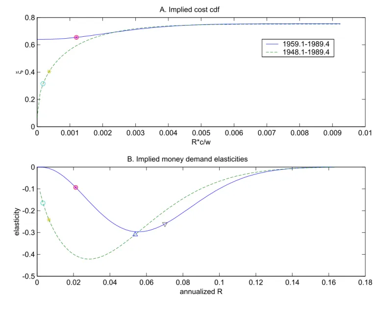
The estimated cost distribution: The parameter estimates over the two sample periods also imply distributions of credit costs, which are displayed in panel A of Figure 2. The first point to note is that the two costs cdfs are very similar for opportunity cost measures exceeding .002, as were the money demand functions in Figure 1. Below this point, the two functions differ substantially. The short sample period suggests that there are many goods (about two-thirds) that have zero credit costs. The longer sample period suggests that there are many more goods with small, but non-neglible transactions costs.
This figure anticipates the results presented below, by indicating not only the lowest interest rate data point as ‘o’ but also the optimal level of the nominal interest rate as ‘*’. For the short sample, the optimal nominal interest rate happens to be virtually identical to the minimum value in the sample, while for the longer sample the optimum is slightly above the minimum value.
The money demand elasticities: Given the cost distribution (45), there is not a single “money demand elasticity”. But we can still compute the relevant elasticity at each point, producing panel B of Figure 2. For the long sample period, the money demand elasticity is less (in absolute value) than one-half and for the short sample period, it is less than one-third. The triangle in panel B indicates the money demand elasticity at the mean interest rate for the sample in question.
Bailey-Friedman calculations. Positive nominal interest rates lead individuals in this model to spend time in credit transactions activity that could be avoided if the nominal interest rate were zero. Given the estimated money demand function, with its associated distribution of credit costs, we can calculate this time cost as h = 0(Rc/w)νdF(ν), which is the area under the inverse money demand function.23
If all goods were purchased with credit, the short (long) sample money demand 22The nonlinear regression chooses the five parameters to minimize the sum of squared errors,
1 T T t=1[ Mt Ptct −(1−F(xt))] 2 with x
t= (Rwtctt)andF(xt) =ξ+ξB(xκt;b1, b2). The point estimates
for the short sample are[ξ=.6394, ξ=.1155,κ=.0127, b1 = 2.8058, b2 = 10.4455]and those for
the long sample are[ξ=.0658, ξ= 0.6859, κ=.0126, b1= 0.4824, b2= 7.1304].
23The “generalized beta” distribution makes this a particularly simple calculation
be-cause the truncated mean of a beta distribution is [ 0yz(z)b1−1(1 − z)b2−1dz]/β(b1, b2) = Γ(b1+1)Γ(b1+b2) Γ(b1)Γ(b1+b2+1)B(y;b1+ 1, b2),so h=κξ Γ(b1+1)Γ(b1+b2) Γ(b1)Γ(b1+b2+1)B( (Rc/w) κ ;b1+ 1, b2).
estimates imply that individuals would spend approximately 0.03% (0.05%) of their time endowment in credit transactions.24 While our estimates are small relative to
those which other researchers have found using aggregate U.S. data, we note that they are less unusual taken in the larger context of money demand studies. For example, using microeconomic data and a different methodology, Attanasio, Jappelli and Guiso [2002] also find relatively low welfare costs of inflation.
6
Optimal policy in the long run
There are two natural reference points for thinking about optimal policy in the long run. The first reference point is Friedman’s [1969] celebrated conclusion that the nominal interest rate should be sufficiently close to zero so that the private and social costs of money-holding coincide. At this point, the economy minimizes the costs of decentralized exchange. The second reference point is an average rate of inflation of zero, which minimizes relative price distortions in steady state. In this section, we document the intuitive conclusion that the long-run inflation rate should be negative — but not as negative as suggested by Friedman’s analysis — when both sticky price and exchange frictions are present.
6.1
The four distortions at zero in
fl
ation
If there is zero inflation in the benchmark economy—which uses the credit cost tech-nology with parameters set from the short sample estimates—then it is relatively easy to determine the levels of the four distortions. With zero inflation, the nominal and real interest rates are each equal to 2.93 percent per annum. The parameters of the credit cost technology imply that 65.6 percent of transactions arefinanced with credit (ξ=.656) and that the ratio of real money to consumption is about 34percent.
The markup is equal to that which prevails in the static monopoly problem, µ= ε
ε−1 =1.11, so that price is roughly eleven percent higher than real marginal cost in
the steady-state.
There areno relative price distortions — allfirms are charging the same, unchang-ing price — so thatδ =1. Further, marginal relative price distortions are also small.
The wedge of monetary inefficiency is positive, but relatively small in this steady 24While this number may seem implausibly small to some readers, reference to Figures 1 and
2 helps understand why it is not given our transactions demand for money. As seen in Figure 1, the largest amount of credit use — implying a rate of money to consumption of about .25 — begins to take place when the opportunity cost is about .005, which translates to an annualized interest rate of just under 10% as seen in Figure 2. With the estimated money demand over the short sample, the money demand curve cuts the axis at less thanm/c=.4, implying an increase in m/c
of.15 =.4−.25. Using a triangle to approximate the integral, we find that the approximate cost saving is 1
state. It is calculated from the above discussion as
(1+ (1−ξ)∗R) = (1+ (1−.656)∗.0072) =1.0025,
where the calculation of the wedge uses the quarterly nominal interest rate .0072. Time costs associated with use of credit are quite small, approximately .004% of the time endowment. Recall that the maximal time costs - associated with using credit for all purchases - are about 0.03%. At zero inflation, time spent on credit transactions involves only 14% of the maximum time that could be spent on credit transactions.
6.2
The benchmark result on long-run in
fl
ation
Even though the distortions associated with money demand are small at zero inflation, a monetary authority maximizing steady-state welfare would nonetheless choose a lower rate of inflation, for the reasons stressed by Friedman [1969]. When we solve the optimal policy problem for the benchmark model using the short-sample estimates displayed in Figure