The Effects of Parameter Tuning on Machine Learning Performance in a Software Defect Prediction Context

(1)

Graduate Theses, Dissertations, and Problem Reports

2015

The Effects of Parameter Tuning on Machine Learning

Performance in a Software Defect Prediction Context

Benjamin N. Province

Follow this and additional works at:

https://researchrepository.wvu.edu/etd

Recommended Citation

Province, Benjamin N., "The Effects of Parameter Tuning on Machine Learning Performance in a Software

Defect Prediction Context" (2015). Graduate Theses, Dissertations, and Problem Reports. 6457.

https://researchrepository.wvu.edu/etd/6457

This Thesis is protected by copyright and/or related rights. It has been brought to you by the The Research

Repository @ WVU with permission from the rights-holder(s). You are free to use this Thesis in any way that is

permitted by the copyright and related rights legislation that applies to your use. For other uses you must obtain

permission from the rights-holder(s) directly, unless additional rights are indicated by a Creative Commons license

in the record and/ or on the work itself. This Thesis has been accepted for inclusion in WVU Graduate Theses,

(2)

The Effects of Parameter Tuning on

Machine Learning Performance

in a Software Defect Prediction Context

Benjamin N. Province

Thesis submitted

to the Statler College of Engineering and Mineral Resources

at West Virginia University

in partial fulfillment of the requirements for the degree of

Master of Science in

Computer Science

with concentration in

Software and Knowledge Engineering

Tim Menzies, Ph.D., Chair

Katerina Goseva-Popstojanova, Ph.D.

Thirimachos Bourlai, Ph.D.

Lane Department of Computer Science and Electrical Engineering

Morgantown, West Virginia

2015

Keywords: Data Mining, Software Defect Prediction, Parameter Tuning,

Machine Learning, Cross-Version Learning, Software Engineering

(3)

ABSTRACT

The Effects of Parameter Tuning on Machine Learning

Performance in a Software Defect Prediction Context

Benjamin N. Province

Most machine learning techniques rely on a set of user-defined parameters. Changes in

the values of these parameters can greatly affect the prediction performance of the learner.

These parameters are typically either set to default values or tuned for best performance

on a particular type of data. In this thesis, the parameter-space of four machine learners is

explored in order to determine the efficacy of parameter tuning within the context of software

defect prediction.

A distinction is made between the typical within-version learning scheme and forward

learning, in which learners are trained on defect data from one software version and used to

predict defects in the following version. The efficacy of selecting parameters based on

within-version tuning and applying those parameters to forward learning is tested. This is done

by means of a cross-validated parameter-space grid search with each tuning’s performance

being compared to the performance of the default tuning given the same data.

For the Bernouli naive Bayes classifier and the random forest classifier, it is found that

parameter tuning within-version is a viable strategy for increasing forward learning

perfor-mance. For the logistic regression classifier, it is found that tuning can be effective within a

single version, but parameters learned in this manner do not necessarily perform well in the

forward learning case. For the multinomial Bayes classifier, no substantial evidence for the

efficacy of parameter tuning is found.

(4)

Acknowledgments

First, I would like to thank my advisor, Dr. Tim Menzies, his colleague Dr. Susan

Partington, the Lane Department of Computer Science and Electrical Engineering, and the

Program of Human Nutrition and Foods for employing me as a GRA for the first year and a

half of my graduate studies and thus providing me with an important source of much-needed

funding.

I would also like to thank the West Virginia Space Grant Consortium, the Jet Propulsion

Laboratory at the California Institute of Technology, and my JPL mentor Justin Lin for

making possible the summer internship which inspired me to pursue graduate studies in the

field of Computer Science as a bridge into the field of intelligent robotics. I would be remiss

not to also thank Dimitris Vassiliadis, the Colorado Space Grant Consortium, and the WVU

department of Physics and Astronomy for their support of RockSat, a program in which I

participated as an undergraduate which put me on the path towards JPL and eventually

graduate school.

I would like to thank my wife, Randy, who helps me to stay focused, and keep my nose to

the grindstone. Without her support, this thesis would have almost certainly taken another

semester to complete.

I would like to thank my parents and grandmother for encouraging my academic success

through childhood and for supplementing my undergraduate scholarships so that I could

avoid the burden of student loans.

I would like to thank my friend Andrew Duncan for his friendship and for sharing some

of his technical expertise. Any time I face a software or electronics challenge that has me

stumped, Andrew is the first person I ask for advice.

Last, but not least, I would like to thank all those who have contributed to Python,

SciPy, NumPy, SciKit-Learn, SPyDEr, Matplotlib, Ubuntu, LinuxMint, MacPorts, L

A

_TEX,

and all the other free software I use. Without free and open-source software, this thesis could

not have happened, and the world would truly be a much less wonderful place.

(5)

List of Figures

3.1 Confusion matrix examples and labels . . . .

18

3.2 g contours as a function of pD, pF . . . .

20

3.3 Confusion Matrix for

m

tests of significance . . . .

37

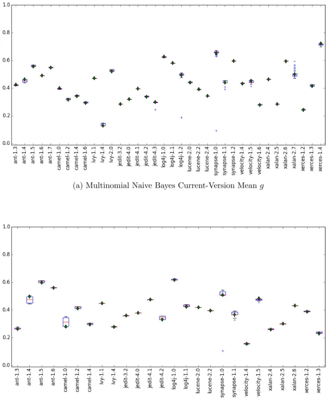
4.1 Multinomial Naive Bayes Mean

g

Box Plots . . . .

44

4.2 Histogram of Logistic Regression Current-Version Successful Tunings

. . . .

46

4.3 Logistic Regression Mean

g

Box Plots . . . .

48

4.4 Histogram of Random Forest Current-Version Successful Tunings

. . . .

50

4.5 Random Forest Mean

g

Box Plots . . . .

52

4.6 Histogram of Bernoulli Bayes Current-Version Successful Tunings . . . .

53

(10)

List of Tables

3.1 CKJM Extended Metrics [17]

. . . .

22

3.2 CKJM datasets of the PROMISE repository . . . .

24

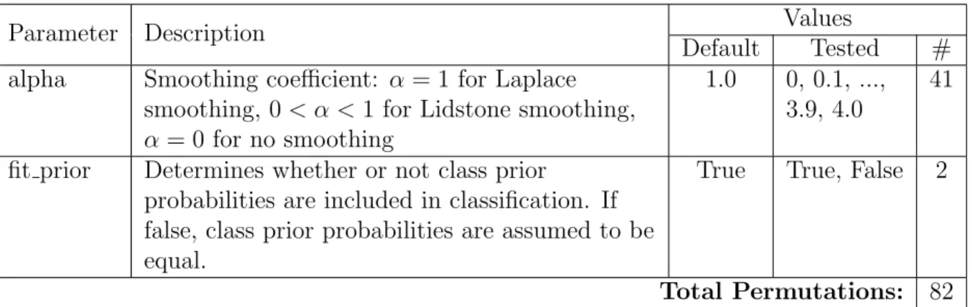
3.3 Sci-kit Learn Multinomial Naive Bayes Parameters

. . . .

27

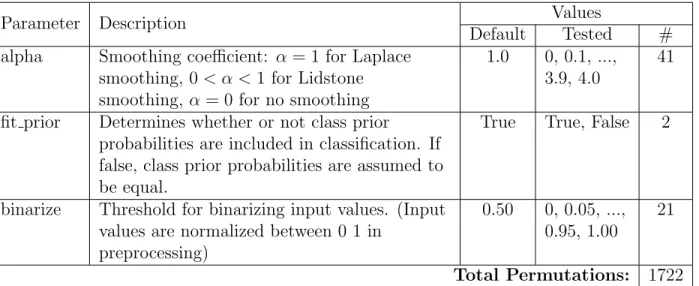
3.4 Sci-kit Learn Bernoulli Naive Bayes Parameters . . . .

28

3.5 Sci-kit Learn Logistic Regression Parameters . . . .

28

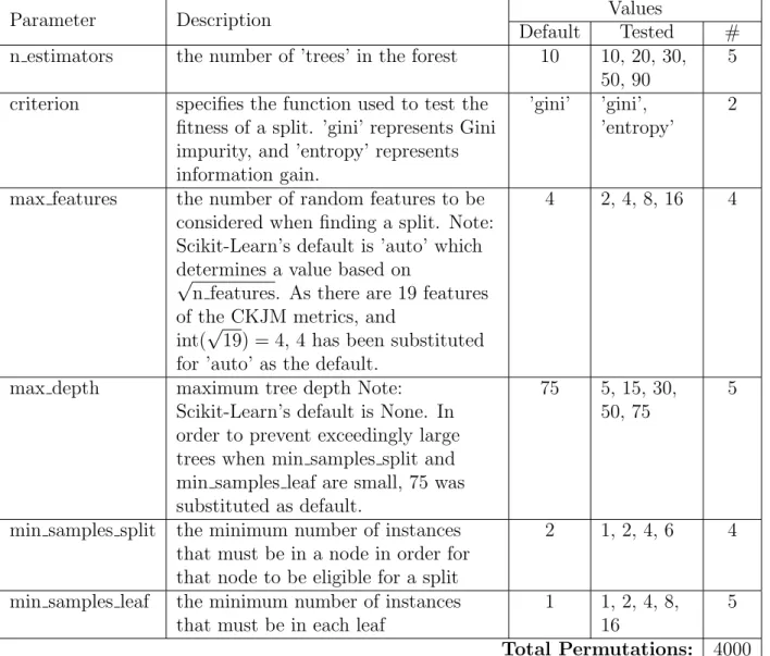
3.6 Sci-kit Learn Random Forest Parameters . . . .

29

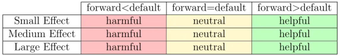
3.7 Version-Forward Learning Outcomes

. . . .

40

3.8 Cohen ’88 Effect Sizes

. . . .

41

3.9 Version-Forward Learning Outcomes by Effect Size

. . . .

41

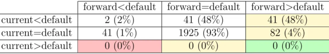
4.1 Version-Forward Learning Outcomes: Multinomial Naive Bayes Total Counts

43

4.2 Version-Forward Learning Outcomes: Logistic Regression Total Counts . . .

47

4.3 Version-Forward Learning Outcomes: Logistic Regression Xalan counts . . .

47

4.4 Version-Forward Learning Outcomes: Random Forest Total Counts . . . . .

50

4.5 Version-Forward Learning Outcomes: Random Forest Total Counts . . . . .

51

4.6 Version-Forward Learning Outcomes: Bernoulli Bayes Total Counts . . . . .

54

(11)

Chapter 1 Introduction

1.1 Motivation

The ultimate end-goal of the work presented in this thesis is the betterment of the quality

of future software. This is a difficult goal to approach as no single solution the software

quality problem exists. As Fred Brooks famously stated “We see no silver bullet. There

is no single development, in either technology or management technique, which by itself

promises even one order of magnitude improvement...” [7] Therefore, the only way to make

progress towards the end-goal of higher quality software is through incremental improvement

to one of a variety of issues with current development practices.

This thesis focuses on one of the major problems plaguing modern software: the

preva-lence of bugs. Although testing and validation are part of most software development cycles,

a shocking number of bugs still make their way into production software to be discovered

by the end-users. The simplistic solution the bug problem is to increase the testing effort

during development. If bugs are caught by developers before the software is released, they

can be fixed before the software is released to end-users. There are several approaches by

which bugs may be caught including extensive unit testing, code walkthroughs, and more

(12)

exhaustive testing of combinations of use cases and options.

The problem with this simplistic approach is that testing consumes resources.

Any

increase in software testing and validation effort will also lead to an increase in overall

development costs and overall development time. Therefore, the trade-off between greater

validation effort and lower development costs is a business decision. Software that has many

bugs will be unappealing, but software that comes at great cost may be equally unappealing.

For this reason, the holy grail of software validation is the development of processes by which

more bugs can be caught without an increase in effort. The real question is how to find bugs

by looking

smarter

rather than

harder

.

A data-mining approach is often used to work towards increasing software quality. In

this approach, various quantifiable statistics or metrics are extracted from the source code

of the software or from the development process. These statistics and metrics are usually

collected for several subsets of a software development project along with the number of bugs

reported for each subset. In this way, hypotheses about the relation between the software

metrics and the likelihood of a bug in the software can be constructed and evaluated. After

a correlation has been established, developers can close the loop by either altering their

development practices to avoid “bad” characteristics or by applying more testing scrutiny

to subsets of the software which exhibit “bad” characteristics.

Data-driven software defect prediction generally relies on machine learning techniques,

most of which have several parameters which can be adjusted to vary the performance of

the learning algorithm. Most machine learners have a default set of parameters which are

chosen by the learner’s creators to reflect the “best” settings for general performance. The

default parameters, however, are not necessarily the top-preforming set of parameters in all

situations. The practice of choosing parameters that lead to increased performance within

a particular domain or when applied to a particular type of data is known as parameter

tuning.

(13)

The intent of this thesis is to explore the practice of parameter tuning, determine it’s

effectiveness in a Software Engineering defect prediction context, and offer insight it’s

effec-tive application. By furthering the understanding of effeceffec-tive parameter tuning, the practice

of software defect prediction can be improved. Improved defect prediction can lead to more

informed software testing, which can contribute to an increase in the overall quality of

soft-ware.

1.2 Research Questions

1) Can within-version parameter tuning lead to increased classification performance on

soft-ware defect data when compared to default parameters?

Each machine learner in Scikit-Learn has a default value for each of its parameters.

The set of default parameter values have been chosen by the authors of Scikit-Learn or the

original developers of the algorithms as a best guess for the appropriate values. It is possible

and even probable that for a given combination of training set and test set, some other

parameter tuning will produce better results than the default tuning. The real question is

weather some parameter tunings preform

significantly

better under repeated re-sampling of

a pool of training and testing data than the default tuning. To explore this question, a

cross-validation study must be preformed and a test of statistical significance must be applied to

the performance results of each non-default tuning.

2) Is parameter tuning effective when the parameters are tuned and the classifier is trained

on data from one version of a software project but tested on the next version?

The main goal of machine learning for defect prediction is that lessons learned from

previously developed software may be applied to software that is currently in development.

Given this goal, it is curious that most defect prediction studies are conducted by sampling

both the training and testing data from the same dataset. This typically comes in the form

(14)

of a cross-validation study where training and testing data are repeatedly resampled from

data reflecting a single version of a single software project. This within-version approach to

tuning evaluation doesn’t fit the business use scenario in which tuning cannot be conducted

on as-of-yet untested versions as class-labels have not yet been established. For example,

it may be that the tunings that yield the best performance when training and testing on

version 1.1 of a software project do not preform as well when the learner is trained on data

from version 1.1 and tested on version 1.2.

3) Is the extent to which a parameter tuning out-performs the default tuning on data from

one software version indicative of it’s likelihood of success in future versions?

This question extends RQ2 by considering effect size. Assuming that tunings that do

well in one software version tend to yield helpful results when they applied to a learner that

is tested on a newer version, does the magnitude of their success matter? It may be that any

tuning which performs better than the defaults when tested on one version is likely to do so

on the next version as well. It may also be that there is some sort of effect size threshold

below which tunings should be ignored. It is important to consider “setting the bar” of how

much better than the defaults a particular tuning must to in one version to be trusted a

subsequent version.

4) Is there a set of parameter tunings that will increase learning performance ubiquitously

in the domain of software defect prediction?

This question has the potential to undo RQs 1 through 3 if it can be answered in the

affirmative. Another way of thinking about it is “If one tuning is consistently doing better

than defaults, why don’t we just change the defaults?” If the tuning experiments keep finding

a particular tuning which out-performs the defaults, then perhaps the defaults were poorly

chosen, or were not set to a value which reflects the best performance within the domain of

software defect prediction. If this is the case, then developers should be made aware of the

“new defaults” and told that implementing parameter tuning in practice is a moot point.

(15)

1.3 Statement of Thesis

The results of the research presented in this thesis can be summarized as follows:

In the context of software defect prediction, parameter tuning is an effective means of

boosting prediction performance of certain machine learning algorithms. For some of these

learners, this holds true not only when they are trained and tested on data from the same

software version, but also when they are tested on future versions not used in training.

This statement is conservatively worded to reflect the fact that parameter tuning does

not produce positive results under

all

circumstances. Based on the evidence in this thesis,

is the position of the author that on the whole, parameter tuning is a worthwhile endeavor.

As parameter tuning is not ubiquitously effective for all learners and all data, trials should

be conducted to judge its effectiveness before applying it in new situations.

(16)

1.4 Structure of Thesis

The remainder of this thesis is organized as follows:

Chapter 2: Background

provides some background information on machine learning

for software defect prediction and parameter tuning of machine learners

Chapter 3: Methods

discusses the machine learning techniques which are used in this

thesis and the means of testing and measuring their predictive performance. It also describes

the data sources used and the method of data selection. Chapter 3 also contains a description

of the design of the experimental trials and finally, descriptions of the statistical methods

employed for comparing results.

Chapter 4: Results

presents the results of this study starting with the learner that

produces the weakest evidence for the efficacy of parameter tuning and progressing to the

learner which produces the strongest evidence for the efficacy of parameter tuning.

Chapter 5: Threats to Validity

presents some observations which may pose a threat

to the validity of the results of Chapter 4 and the generalizability of the conclusions in

Chapter 6. Chapter 6: Conclusions and Suggestions for Implementation

summarizes the

findings of this thesis and provides some suggestions for the practical implementation of

parameter tuning techniques within the context of software defect prediction.

(17)

Chapter 2 Background

2.1 Simple Methods Work Well for Defect Prediction

While training a classifier on previous examples, there may be overfitting problems for

com-plex learning schemes. It is a repeated result in Software Engineering defect prediction that

simplistic methods seem to work about as well as more complicated methods. This is why

in their 2012 review of fault prediction literature, Hall et al. concluded that “models which

perform well tend to use simple, easy to use modeling techniques like Naive Bayes or Logistic

Regression. More complex modeling techniques, such as Support Vector Machines, tend to

be used by models which perform relatively less well.“ [12] In addition, Menzies et al. have

shown that there is a ceiling effect of sorts when dealing with SE defect prediction. [21] This

means that machine learners tend to get about as good of results when training on a small

subset of the instances in the training set.

(18)

2.2 Parameter Tuning of Machine Learners

The tuning of parameters of machine learning algorithms is not a new concept. In

litera-ture, the general process of parameter tuning is sometimes referred to as “hyperparameter

optimization”. The term “hyperparameter” is used in the context of statistical model fitting

to refer to a parameter governing shape of the assumed prior distribution of data. This

distinguishes it from parameters which are internal to the model which are scaled to achieve

the best fit. In this thesis, some, but not all parameters explored fit this strict definition of

“hyperparameter”, so the more general term “parameter tuning” is used instead of

“hyper-parameter optimization”

The most commonly discussed methods of parameter tuning are grid search and random

search. Other more sophisticated methods have been proposed which intelligently search the

parameter space, choosing new sets of test parameters based on the performance of previous

trials. These methods have a few drawbacks when compared to random search and grid

search. They generally assume some continuity of performance throughout the parameter

space, which may not be true. [5] These iterative search methods are also often difficult to

parallelize.

Grid search is a simpler method of parameter optimization that is resistant to

disconti-nuities and nonlinearities provided that the grid is sufficiently fine. It is easily parallelizable

and simple to understand, but is also generally regarded as the most computationally

ex-pensive method of parameter tuning. Interestingly, Bergstra and Bengio have shown that

given the same computational time, a random search is likely to find a better-performing

parameter tuning than a grid search with the same bounds. [4] This makes random search

an attractive method of parameter tuning for practice, but for reasons of repeatability this

thesis will focus on grid search for parameter optimization.

(19)

2.3 Parameter Tuning in Evolutionary Algorithms

Aside from classification algorithms, parameter tuning is also used for other complex

algo-rithms including regression, computer vision, and evolutionary algoalgo-rithms. The literature on

tuning of evolutionary algorithms is relatively vast, possibly due to the large computation

costs associated with random or grid search of their parameter spaces. Some of these

evolu-tionary algorithm results are of particular interest here due to their use in a closely related

domain: search-based Software Engineering.

Search-based Software Engineering (SBSE) is a different type of machine learning. Where

defect prediction data mining is concerned with creating predictive models of software

de-fects, SBSE is concerned with finding optimal solutions to a given model. In other words, a

search of the model’s input space is conducted in order to find input-values corresponding

to a desired output. SBSE often relies on a genetic algorithms approach to search due to

the complexity of the models.

In 2011, Arcuri and Fraser explored the effects of parameter tuning of genetic algorithms

in a SBSE context. They found that “Different parameter settings cause very large variance

in the performance.” and that “Default parameter settings perform relatively well, but

are far from optimal on individual problem instances.”. [1] In this thesis, these conclusions

are found to be generally extensible to the software defect prediction context with a few

exceptions.

In a paper that is not software engineering specific, Smit and Eiben compared three

parameter tuning strategies for evolutionary algorithms and found that they all produced

parameter values that yielded performance superior to that of manual human-in-the-loop

tuning. [33] They also found in a survey of tuning literature that the “tunability” of

param-eters may vary from algorithm to algorithm and dataset to dataset but that “The efforts [of

tuning] are moderate and the gains in performance can be very significant.” [11]

(20)

Chapter 3 Methods

3.1 Machine Learning Techniques

Various machine learning techniques have been designed to solve the problem of

classifica-tion. In order to apply a classification technique, the features which have been extracted

from the software data must be mapped into the domain required for the learner’s inputs.

This may require pre-processing that converts numeric values into categorical values such as

high/med/low or the assignment of categorical values to integer representations depending

on the cardinality of the data and the requirements of the learning scheme.

This thesis will explore the effects of parameter tuning on three types of machine learners:

Bayesian classifiers, logistic regression, and the random forrest classifier. It is important to

understand the basics of each of these machine learning techniques before we can explore

their parameter spaces. While each of these techniques has been discussed at length and with

great depth in machine learning literature, this section merely aims to provide an overview

of each of these methods.

(21)

3.1.1 Bayesian Classification

Bayesian classification is one of the oldest, simples, and most widely used machine learning

techniques ever developed. Several variants of Bayesian classification schemes exist, but

the premise of all Bayesian classifiers is the same: the application of Bayes’ Rule. When

expressed in terms of a single datum of evidence

E

, the Bayesian probability of a single class

outcome

C

is given as

p

(

C

|

E

) =

p

(

C

)

· p

(

E

|

C

)

p

(

E

)

(3.1)

where

p

(

C

|

E

) is the probability of particular classification given the evidence,

p

(

C

) is the

prior probability of the classification,

p

(

E

|

C

) is the likelihood of observation

E

within

train-ing examples of class

C

, and

p

(

E

) is the prior probability of the evidence. [37]

In a Bayesian classifier, the goal is not to determine the

actual probability

of a single

class, but rather to chose the

most likely

class from a set of possible classifications. In this

case, let ˆ

i

be the most likely class from the set

{

C

0 , C

1 , ..., C

n

}

given evidence

E

. Under

these conditions, the most likely class given the evidence can be expressed as

ˆ

_i

_{= arg max}

i

∈{0

,

1 ,...,n

}

p

(

C

i

)

· p

(

E

|

C

i

)

p

(

E

)

(3.2)

It should be noted that this expression assumes a single datum of evidence. In order to be

useful as a classifier, equation equation 3.2 must be modified to support a set of evidence

such that

E

=

{

E

0 , E

1 , ..., E

k

}

. This presents two challenges. Firstly, a specific combination

of evidence may not exist in training data. This means that

p

(

E

) would become zero. In

order to prevent this,

p

(

E

) can be removed from the equation because it is a constant across

for all

C

i

evaluated within the argmax. This simplification yields:

ˆ

_i

_{= arg max}

i

∈{0

,

1 ,...,n

}

p

(

C

i

)

· p

(

E

0 , ..., E

k

|

C

i

)

(3.3)

(22)

is the expansion of

p

(

E

0 , ..., E

k

|

C

i

). Under the chain rule for conditional probabilities:

p

(

E

0 , ..., E

k

|

C

i

) =

p

(

E

0 |

C

i

)

· p

(

E

1 |

E

0 , C

i

)

· p

(

E

2 |

E

1 , E

0 , C

i

)

· ...

· p

(

E

k

|

E

k

−1

, ..., E

0 , C

i

) (3.4)

This is where the “naivety” of a naive Bayes classifier comes in to play. In order to simplify

equation 3.4, an assumption of independence between the evidence variables is made. If

each element of the evidence is assumed to be independent from each other element (which

may or may not hold true) then the conditions for each probability in equation 3.4 can be

reduced to

C

i

such that:

p

(

E

0 , ..., E

k

|

C

i

) =

p

(

E

0 |

C

i

)

· p

(

E

1 |

C

i

)

· p

(

E

2 |

C

i

)

· ...

· p

(

E

k

|

C

i

) =

k

Y

j

=0

p

(

E

j

|

C

i

)

(3.5)

Plugging equation 3.5 into equation 3.3 yields the final simplified equation for the class

predication of a naive Bayes classifier using a discrete set of evidence. [15]

ˆ

_i

_{= arg max}

i

∈{0

,

1 ,...,n

}

p

(

C

i

)

k

Y

j

=0

p

(

E

j

|

C

i

)

(3.6)

Gaussian Bayes Classifier

One way to modify the Bayesian classifier for continuous numeric features is to assume that

the distribution of values for each feature is Gaussian. In this way, the probability of each

feature value for a given class can be expressed as:

P

(

E

j

|

C

i

) =

1 p

2 πσ

2 C

· exp

−

(

E

j

−

µ

C

)

2

2 σ

2 C

(3.7)

where

µ

C

and

σ

C

are the mean value and standard deviaiton of

E

j

seen in training instances

of class

C

i

. [35]

(23)

Multinomial Bayes Classifier

The Multinomial Bayses classifier addresses the problem of missing values through

smooth-ing. It adds a small value,

α

, to the count of each feature when computing the probability

such that all combinations of features and classes have a non-zero probability. This process

is called Laplace smoothing when

α

= 1 and Lidstone smoothing when

α <

1. The smoothed

feature values are given as:

ˆ

E

Cj

=

E

Cj

+

α

E

C

+

αn

(3.8)

where

E

Cj

is the sum of all values of feature

j

given class

C

seen in training,

E

C

is the

sum of

E

Cj

for all classes, and

n

is the number of features. Multinomial Bayes classifier is

primarily used in text mining where the features are word counts, which may be sparse. [30]

Bernoulli Bayes Classifier

The Bernoulli Bayes classifier assumes the special case that all features are binary-valued.

For numeric features, this requires a binarization pre-processing step. [35] For Bernoulli

Bayes, the probability of each feature value for a given class can be expressed as:

p

(

E

j

|

C

i

) =







E

j

:

p

(

j

|

C

i

)

¬

E

j

: 1

−

p

(

j

|

C

i

)

(3.9)

This provides a case for explicitly handling missing features, rather than ignoring them,

though the smoothing technique described for Multinomial Bayes can also be applied.

When using numerically valued data is being used with a Bernoulli Bayes classifier, it

must be pre-processed to meet the binary value assumption.

This is typically done by

normalizing each dataset attribute and then applying a binarization threshold. For this

thesis, any data which is being passed to a Bernouli Bayes classifier is normalized by shifting

and linearly scaling such that the minimum and maximum values of each attribute are 0 and

(24)

1 respectively. A binarization threshold between 0 and 1 is then used as a parameter of the

learner.

3.1.2 Random Forest Classifier

The random forest classifier is an ensemble method in which a “forest” of several decision tree

classifiers is created. At each node of each decision tree, the best feature on which to split

the tree is chosen from a random subset of available features. These best feature on which

to split the decision tree is typically selected such that a split would either minimize the

node’s Gini impurity or maximize the node’s information gain relative to all other features

available for the split. Each decision tree continues to be split until a stopping criteria such

as maximum depth or minimum training instances is reached, or the class of all training

data for a given node is homogenous. [6]

In addition to the random subsamples of the feature space at each node of each decision

tree, some random forest implementations also reduce overfitting by bootstrap sampling the

training data to be used on each tree. In this way, if there are

n

instances of training data,

each tree will be trained on

n

instances randomly sampled with replacement from the original

training data.

After a random forest has been trained, new examples can be classified by traversing

each of the individual decision trees until a leaf is reached. The majority class of the leaf

reached in each decision tree is that tree’s “vote” and the class with the most votes among

all trees in the forest is the classifier’s prediction.

3.1.3 Logistic Regression

Regression-based algorithms have the advantage of natively handling continuously defined

numeric inputs. When using a regression for classification, some allowances must be made

(25)

due to the discrete nature of the defendant variable. One clean way to handle this is by using

the logistic function as the basis for regression. The logistic function’s range is asymptotically

bounded between 0 and 1, which makes it useful for modeling probabilities. The logistic

function is given as:

σ

(

t

) =

e

t

e

t

_{+ 1}

=

1 1 +

e

−

t

(3.10)

The probability of a boolean classification such as the presance of a software bug being

“true”,

p

(

C

|

E

), can be modeled as a logistic function given that

t

is a linear combination of

evidence and weights such that:

p

(

C

|

E

) =

σ

(

t

)

where

t

=

β

0 +

β

1 E

1 +

β

2 E

2 +

...

+

β

k

E

k

(3.11)

In this way, the classifier can be trained by finding the values of

β

0 , β

1 , ...

which best fit the

probability of C in training data. [29] In order to do this, we must consider the inverse of

logistic function: the logit function. Applying equation 3.11 to the logit function yields:

g

(

E

) =

ln

p

(

C

|

E

)

1 −

p

(

C

|

E

)

=

β

0 +

β

1 E

1 +

β

2 E

2 +

...

+

β

k

E

k

(3.12)

The

β

coefficients from equation 3.12 can be estimated from the training data using an

maximum likelihood estimator and an iterative solving technique such as Newton’s method.

[23] This can lead to overfitting issues which can be mitigated by using regularization. This

is typically done using L1 (lasso) or L2 (ridge) regularization. In both cases an extra term

reflecting the complexity of the fit is added to the loss equation for the least-squares fit. In

L1 regularization, the extra loss term is the sum of the absolute values of all

β

coefficients,

while in L2 regularization, the extra loss term is the geometric sum of all

β

coefficients,

which is equivalent to the magnitude of the

β

vector. [24] This loss term is scaled through

multiplication by a parameter of the learner called “regularization strength”.

(26)

lo-gistic regression. This transforms the minimization problem into a transposed maximization

problem which results in the same optimal coefficients. Solving the dual problem is more

computationally efficient when the evidence set is sparse, or where there are more evidence

features than there are instances in the training set. [36]

3.2 Evaluating Machine Learning Performance

The general process of evaluating the performance of a machine learner involves two datasets:

a training set and a test set. The classifier uses the training set as a pool of examples from

which to draw inference. This means that each datum within the training set must have a

class label which is know a-priori. Once a learner instance has received several examples in

the form of a training set, it is considered a

trained

classifier.

After a classifier is trained, its performance can be tested by attempting to classify

examples from the test set. The test set is passed to the learner

without

class labels, and

the learner returns the class which to which each example is most likely to belong based

on the training examples and the principles governing the classifier’s behavior. In a

real-world classification situation, the class labels of the test set may not yet be known; it is

the classifier’s job to determine the label. When evaluating the performance of a classifier,

however, the actual class labels of the test set must be known so that the classifier’s predicted

labels can be compared to the ground-truth labels.

In order to compare the performance of multiple machine learners, meaningful numeric

measures of performance must be chosen. In this case, a performance measure is any way

of assigning a number to measure how well a classifier’s predicted classes for the test set

match up with the ground-truth classes. This step is important because some measures,

such as accuracy, may not tell the whole story of performance depending on the nature of

class distributions within the test set.

(27)

Another consideration for establishing the performance of a given learner on a given

dataset is how to partition the set into training and testing sets. When preforming a single

trial with one train/test partition, the learner’s performance may be sensitive to the chosen

partition. A better way to handle this is the LOO (leave one out) method. In LOO, a

separate learning trial is conducted for each individual datum in which the selected datum

is used as a test set and the rest of the data constitutes the training set. LOO can be

impractically computationally expensive, so a subsampling method called stratified k-fold

cross-validation with repeats is employed here instead. Cross-validation will be explained

below in section 3.4.2.

3.2.1 Confusion Matrices

Before discussing classification performance measures, it is useful to discuss the concept of a

confusion matrix. Confusion matrices show the number of items of each class that a classifier

predicts to be each other class. Each row in a confusion matrix represents a true class while

each column represents a predicted class. (See Figure 3.1 for examples) In the case of 100%

accurate prediction, the confusion matrix should be a diagonal matrix as all predictions

match the ground-truth. The number of rows and columns in a confusion matrix are equal

to the number of possible classes represented, which may be any whole number of two or

greater.

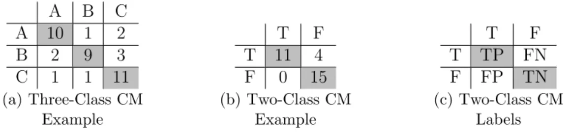
For the special case of a two-class problem, in which the only possible outcomes can be

represented as positive and negative (or true and false), the confusion matrix consists of

only four squares which can be labeled TP (True Positive), FP (False Positive), TN (True

Negative), and FN (False Negative). In this category system, the terms “positive” and

“negative” refer to the predicted classification and the terms “true” and “false” indicate

whether or not the predicted classification was correct. For a visual representation of these

labels, see Figure 3.1c.

(28)

Figure 3.1:

Confusion matrix examples and labels.

Rows represent ground-truth and

columns represent predicted classes. Shaded squares represent correct predictions. TP, TN,

FP, and FN represent True Positive, True Negative, False Positive, and False Negative

re-spectively.

A

B

C

A

10

1

2 B

2

9

3 C

1

11 (a) Three-Class CM

Example

T

F

T

11

4 F

0

15 (b) Two-Class CM

Example

T

F

T

TP

FN

F

FP

TN

(c) Two-Class CM

Labels

Software bug detection can be represented as a two-class problem in which the presence

of a bug is considered “positive” and the absence of a bug is considered “negative”. Although

more classes could be used to represent different types of bugs or bugs which were reported

or treated in different ways, it is useful to represent the presence of a bug as a two-class

problem. Restricting the number of classes to two increases performance by reducing the

number of categories between which a classifier must differentiate and also allows the use

of performance measures such as “probability of detection” which have little meaning when

there are more than two classes.

3.2.2 Measures of Classification Performance

In order to evaluate the efficacy of machine learners, some measurements need to be applied

to the confusion matrix yielded from the testing of a trained classifier. For most machine

learning circles, the typical performance evaluation metrics are precision and recall. Within

the domain of Software Engineering defect prediction, the majority of the recent publications

favor pD (probability of detection) and pF (probability of false-alarm). This is largely due

to scaling issues with precision that arise when the testing data has positive/negative ratios

near 0 or 100%. [20]

(29)

can be expressed as the number of true positives divided by the total number of positive

cases, while pF can be expressed as the number of false positives divided by the total number

of negative cases.

pD

= recall =

# of defects correctly predicted

# of actual defects

=

T P

+

F N

(3.13)

pF

=

# of false defect predictions

# of non-defective items

=

F P

+

T N

(3.14)

This thesis will focus primarily on pD and pF as the chief metrics for comparing machine

learning results because they are business-intuitive for defect prediction and because they

are in line with recent publications. The goal is to have the highest possible pD and the

lowest possible pF, but there is often a trade-off between the two based on the parameters

chosen for a given classification scheme.

In order to effectively rank results it is useful to have a single metric which reflects

overall performance, but neither pD or pF is sufficient on their own. As an example, a

dummy classifier which always predicts “true” is going to have a pD of 100% but will also

have a pF of 100%. Conversely, a dummy classifier which always predicts “false” will have

a pF of 0, which is excellent, but will also score 0 on pD, making it useless. Consequently,

we can define a “no information” line on a pD, pF plot where pD=pF. A dummy classifier

which guesses positive

n

% of the time and negative 100

−

n

% of the time is expected to have

a performance along this line. For a visual representation of the line of no information, see

figure 3.2.

In order to reflect overall performance, a synthetic metric will be used. A typical synthetic

metric for combining precision and recall is the balance F-score which is the harmonic mean

of precision and recall. In this case, as we are focusing on pD and pF, a similar metric, g,

will be used where g defined as the harmonic mean of pD and 1-pF.

(30)

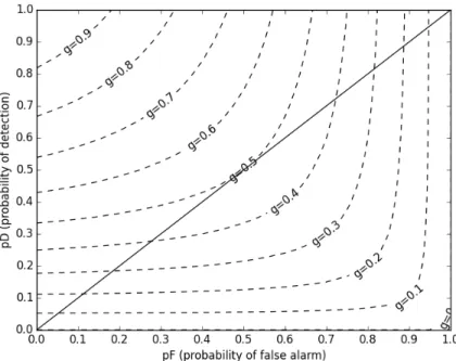
Figure 3.2:

g contours as a function of pD, pF. The solid line represents the line of no

information, the expected performance from random guess.

g

=

₁

2 pD

+

1 1−

pF

=

2(

pD

)(1

−

pF

)

1 +

pD

−

pF

(3.15)

A contour plot of the values of g based on pD and pF can be seen in figure 3.2.

3.3 Data

3.3.1 Data Sources

Some companies keep records of completed software projects which may be used to learn

lessons for future development. These software companies have little incentive to release

their development data to the general public. Most Software Engineering researchers rely

on public data from various sources including the PROMISE repository [22], a engineering

project data repository supported by North Carolina State University.

(31)

The PROMISE repository includes many Software Engineering defect and effort

pre-diction datasets from previous software projects.

The software project data hosted on

PROMISE has features which are measured with a variety of different types of software

metrics. Many of these software projects have data available on PROMISE from multiple

versions.

In the interest of openness an reproducibility of results, only data publicly available on

the PROMISE dataset will be used in this thesis. In addition, to this restriction, the data

used in this thesis will also be restricted to software projects for which three or more versions

(numbered releases) are available. This will allow for the evaluation of cross-version learning.

Another necessary restriction is that the software metrics used be homogenous to ensure fair

comparison. To this end, only software projects using the CKJM object-oriented metrics

will be considered as choosing CKJM metrics allows for the largest plurality of datasets to

be included when considering the first two restrictions.

3.3.2 CKJM Metrics

CKJM (Chidamber and Kemerer Java Metrics) is a tool for tabulating the object-oriented

software metrics devised by Chidamber and Kemerer [8] for given Java classes. An updated

version of CKJM, called CKJM Extended, also tabulates several other object-oriented

soft-ware metrics on a per-class basis. [17] CKJM Extended includes Henderson-Sellers’ LCOM3

metric [13], Martin’s afferent and efferent couplings [18], Bansiya Davis’ QMOOD metrics [2],

Tang, Kao, and Chen’s coupling and complexity metrics [34], and McCabe’s cyclomatic

com-plexity measure [19] as well as the original Chidamber and Kermer metrics and lines of code

(LOC). For descriptions of all CKJM Extended metrics, see Table 3.1.

Several open source Java projects were analyzed by Jureczo and Spinellis using CKJM

Extended, and a dataset was constructed from each version of each project. [17] These

datasets consisted of the CKJM Extended metrics as well as a class variable indicating

(32)

Table 3.1:

CKJM Extended Metrics [17]

Name Description Source

Weighted methods per class (WMC)

The value of the WMC is equal to the number of methods in the class (assuming unity weights for all methods).

C&K [8]

Depth of Inheritance Tree (DIT)

The DIT metric provides for each class a measure of the inheritance levels from the object hierarchy top.

C&K [8]

Number of Children (NOC)

The NOC metric simply measures the number of immediate descendants of the class. C&K [8] Coupling

between object classes (CBO)

The CBO metric represents the number of classes coupled to a given class (efferent couplings and afferent couplings). This couplings can occur through method calls, field accesses, inheritance, method arguments, return types, and exceptions.

C&K [8]

Response for a Class (RFC)

The RFC metric measures the number of different methods that can be executed when an object of that class receives a message. Ideally, we would want to find for each method of the class, the methods that class will call, and repeat this for each called method, calculating what is called the transitive closure of the method call graph. This process can however be both expensive and quite inaccurate. Ckjm calculates a rough approximation to the response set by simply inspecting method calls within the class method bodies. The value of RFC is the sum of number of methods called within the class method bodies and the number of class methods. This simplification was also used in the Chidamber and Kemerer’s description of the metric.

C&K [8]

Lack of cohesion in methods (LCOM)

The LCOM metric counts the sets of methods in a class that are not related through the sharing of some of the class fields. The original definition of this metric (which is the one used in ckjm) considers all pairs of class methods. In some of these pairs both methods access at least one common field of the class, while in other pairs the two methods do not share any common field accesses. The lack of cohesion in methods is then calculated by subtracting from the number of method pairs that do not share a field access the number of method pairs that do.

C&K [8] Lack of cohesion in methods (LCOM3)  1_a 10 P j=1 µAj  −m 1−m

m- number of procedures (methods) in class

a- number of variables (attributes) in class

µ(A) - number of methods that access a variable Henderson-Sellers [13] Afferent

couplings (Ca)

The Ca metric represents the number of classes that depend upon the measured class. Martin [18] Efferent

couplings (Ce)

The Ca metric represents the number of classes that the measured class is depended upon. Martin [18] Number of

Public Methods (NPM)

The NPM metric simply counts all the methods in a class that are declared as public. The metric is known also as Class Interface Size (CIS)

QMOOD [2]

Data Access Metric (DAM)

This metric is the ratio of the number of private (protected) attributes to the total number of attributes declared in the class.

QMOOD [2] Measure of

Aggregation (MOA)

This metric measures the extent of the part-whole relationship, realized by using attributes. The metric is a count of the number of class fields whose types are user defined classes.

QMOOD [2]

Measure of Functional Abstraction (MFA)

This metric is the ratio of the number of methods inherited by a class to the total number of meth-ods accessible by the member methmeth-ods of the class. The constructors and the java.lang.Object (as parent) are ignored.

QMOOD [2]

Cohesion Among Methods of Class (CAM)

This metric computes the relatedness among methods of a class based upon the parameter list of the methods. The metric is computed using the summation of number of different types of method parameters in every method divided by a multiplication of number of different method parameter types in whole class and number of methods.

QMOOD [2]

Inheritance Coupling (IC)

This metric provides the number of parent classes to which a given class is coupled. A class is coupled to its parent class if one of its inherited methods functionally dependent on the new or redefined methods in the class.

Tang [34]

Coupling Between Methods (CBM)

The metric measures the total number of new/redefined methods to which all the inherited methods are coupled. There is a coupling when at least one of the given in the IC metric definition conditions is held.

Tang [34]

Average Method Complexity (AMC)

This metric measures the average method size for each class. Size of a method is equal to the number of Java binary codes in the method.

Tang [34]

McCabe’s cyclomatic complexity (CC)

CC is equal to number of different paths in a method plus one. Max(CC) - the greatest value of CC among methods of the investigated class

Avg(CC) - the arithmetic mean of the CC value in the investigated class

McCabe [19]

Lines of Code (LOC)

The LOC metric based on Java binary code. It is the sum of number of fields, number of methods and number of instructions in every method of the investigated class.

(33)

whether a bug was present in each Java class and if that bug was fixed or not. It should

be noted that “class variable” refers to the classification of a bug being present, and may

be potentially confused with a Java class. In this case, each Java class in each version of

each project has 19 metric features and one class variable indicating the presence or lack

thereof of a bug. The datasets that Jureczo and Spinellis constructed in this manner were

contributed to the PROMISE repository. Several of these data are used in this thesis.

3.3.3 Data Selection

In summary, the criteria for the selection of data which can help answer the research questions

are as follows:

1. The data sets must have a ground-truth class which indicates the presence or absence

of a bug in each software module.

2. All datasets selected must have homogenous feature types. In other words, the same

software metrics must be present in all datasets.

3. For each software project selected, there must be available datasets reflecting the

de-velopment of multiple versions.

4. All selected data must be available for study and replication

In order to meet requirement 4, data is selected from the PROMISE repository, which is

publicly available at http://openscience.us. [22] In order to meet requirement 1, only defect

prediction data will be considered. In order to meet requirement 2 while allowing the largest

quantity of projects meeting requirement 3, only the CKJM-featured defect data will be

considered for selection. A list of these datasets can be seen in Table 3.2

(34)

Table 3.2:

CKJM datasets of the PROMISE repository

Project

Versions

Selected

Ant

1.3, 1.4, 1.5, 1.6, 1.7

Yes

Arc

1 No

Berek

1 No

Camel

1.0, 1.2, 1.4, 1.6

Yes

CKJM

1 No

e-Learning

1 No

Forrest

0.6, 0.7, 0.8

No

Intercafe

1 No

Ivy

1.1, 1.4, 2.0

Yes

Jedit

3.2, 4.0, 4.1, 4.2, 4.3

Yes

Kalkulator

1 No

Log4j

1.0, 1.1, 1.2

Yes

Lucene

2.0, 2.2, 2.4

Yes

Nieruchomosci

1 No

Pbeans

1, 2

No

Pdftranslator

1 No

Poi

1.5, 2.0, 2.5, 3.0

No

Prop

1, 2, 3, 4, 5, 6

No

Redaktor

1 No

Serapion

1 No

Synapse

1.0, 1.1, 1.2

Yes

Systemdata

1 No

Szybkafucha

1 No

Termoproject

1 No

Tomcat

1 No

Velocity

1.4, 1.5, 1.6

Yes

workflow

1 No

wspomaganiepi

1 No

Xalan

2.4, 2.5, 2.6, 2.7

Yes

Xerces

1.0, 1.2, 1.3, 1.4

Yes

Zuzel

1 No

(35)

3.4 Experimental Design

In order to experiment with parameter tuning, a set of Python scripts were developed for

evaluating the performance of four different classifiers: the Multinomial Bayes, the Bernoulli

Bayes, logistic regression, and random forests. In order to reduce the possibility of errors in

the implementation of these learners and to facilitate reproducibility, SciKit-Learn’s Python

implementation of these learners was used. [28]

The

Dataset

class used in this project to manage the data and dataset attributes was

re-used from the work of Vasil Papakroni’s masters work in the development of a machine

learning algorithm called PEEKING2. [27]

A Python package called “BenTune” was created for the purpose of this thesis which

in-cludes, among others, a

Learner

class and a subclass for each of the selected learners which.

The

Learner

classes act as front-ends for the SciKit-Learn learners, accepting training and

testing data in the form Paporkoni’s

Dataset

objects and parameter dictionaries in a

consis-tent format. The

Learner

objects then initialize the SciKit-Learn learners in the appropriate

ways for each individual learner with parameters reflecting the

Learner

’s parameter values

and with training data coerced from the

Dataset

object into the proper format for the learner.

After initializing and training their Scikit-Learn learner, the

Learner

objects then evaluate

its performance by coercing each row of the testing

Dataset

object into a format appropriate

for the learner, and soliciting a prediction of that row’s class. These predictions along with

the ground-truth value for each row are used to initialize an object of the

Results

class, which

is also implemented as part of BenTune.

The

Results

class contains methods for computing confusion matrices and performance

metrics based on the pairs of ground-truth and predicted class values.

Results

also contains

methods for combining with other results to form aggregations. In this way, a

Results

tree

can be formed. Non-leaf nodes in such a tree can be statistically compared to other nodes

(36)

of the same height using their children samples.

The general experimental design of this thesis is that the classes described above are

manipulated in such a way as to conduct a grid-search of the parameter space of each

selected learner. Each parameter tuning evaluated is done so using a 5-fold, 5-repeat,

class-stratified cross-validation. The results of these cross-validation trials are each individually

compared to the default tuning using a test of statistical significance. This is done in two

different evaluation schemes, current-version and forward evaluation. Afterwards, the results

are analyzed. Each of these individual steps is described in greater detail in the following

sections.

3.4.1 Parameter Grid Search

For the sake of relative completeness, a grid search method is used for finding parameter

tunings which out-preform the default parameters. In a grid search, a list of possible values

for each parameter of each learner is constructed, then all combinations of each listed

param-eter value are exhaustively tested. For discretely-valued paramparam-eters with a finite number of

valid values, this is a simple matter of listing all valid parameter values. For parameters in

a continuous regime, the definition of a list of values to be explored is somewhat arbitrary.

When selecting discrete parameter values from continuous ranges, it is tempting to define

a minimum sensible value and a maximum sensible value and explore 100 values between the

minimum and maximum spaced at regular intervals. However, as a mater of pragmatism,

one must remember that the total computation time for a grid-search of all parameter

per-mutations is an exponential problem. If a learner has three continuously-valued parameters

and each is tested at 100 discrete values, the total number cross-validated trials required

to test all parameter permutations is 100

3 _{= 1}

_million

_{trials. More practically, if the same}

three parameters are discretized into ten values each, a much more reasonable 10

3 = 1000

trials are required.

(37)

Table 3.3:

Sci-kit Learn Multinomial Naive Bayes Parameters

Parameter

Description

Values

Default

Tested

#

alpha

Smoothing coefficient:

α

= 1 for Laplace

smoothing, 0

< α <

1 for Lidstone smoothing,

α

= 0 for no smoothing

1.0 0, 0.1, ...,

3.9, 4.0

41 fit prior

Determines whether or not class prior

probabilities are included in classification. If

false, class prior probabilities are assumed to be

equal.

True

True, False

2 Total Permutations:

82 In order to keep the parameter space small enough to be practically explored in a grid

search, some decisions must be made about which values to explore for each

continuously-valued parameter. These choices are the product of a rational line of reasoning, but can

not, by their nature, be defended against all alternate sets of values which might have been

explored instead. For instance, if

{

2 ,

4 ,

6 ,

8 }

is chosen as a rational set of values to be

explored for a given parameter, it can not be argued to be any better or worse of a choice

than

{

2 .

1 ,

4 .

1 ,

6 .

1 ,

8 .

1 }

or

{

1 .

9 ,

3 .

9 ,

5 .

9 ,

7 .

9 }

would have been.

For each learner which was tested, the parameter values used and their default values

are listed in Tables 3.3 through 3.6. For the most part, default values from Sci-Kit learn’s

documentation were used as defaults for this project. In the case of two Random Forest

pa-rameters, the defaults were modified, but not in ways which would greatly effect performance.

For more details on this substitution, see Table 3.6.

For Logistic Regression, when use of one parameter value precludes certain values of other

parameters, the original SciKit-Learn values were modified. This was done in two instances.

In the first one, Logistic regression originally had a

penalty

parameter which could be set

to ’l1’ or ’l2’ and a

dual

parameter which could be set to True or False, but could only be

True if

penalty

was set to ’l2’. To simplify this, the intermediate LogisticRegression class

which calls the SciKit-Learn logistic regression learner accepts only the

penalty

parameter,

but with values of ’l1’, ’l2’, or ’l2 dual’ and sets SciKit-Learn’s

penalty

and

dual

parameters