Copula-Based
Precipitation Fields Estimation
Combining Data
From Radar, Gauge And
Microwave Attenuation
Dissertation
zur Erlangung des Doktorgrades an der
Fakultät für Angewandte Informatik
der Universität Augsburg
vorgelegt von
Wei Qiu
aus
China
Master of Science (ESPACE), TU München
2012
Erstes Gutachten:
Prof. Dr. Harald Kunstman
Zweites Gutachten:
Prof. Dr. Jucundus Jacobeit
Weiteres Gutachten:
Prof. Dr. Karl-Friedrich Wetzel
Tag der mündlichen Prüfung: 30.07.2012
acknowledgements
In the first place, I want to express my sincere gratitude to Prof. Dr. Harald Kun-stmann for offering me the opportunity to work on the challenging topic about using Copula-based approaches to estimated precipitation fields combining data from vari-ous observation devices. Without his enlightening instruction, impressive kindness and patience, I could not have completed my thesis. From numerous discussions with him, what I have learned is not only the scientific knowledge, but also the way of thinking about research, which is invaluable for my future academic career.
My special thanks go to Dr. Stefanie Vogl and Dr. Patrick Laux for their generous helps since I started to learn the Copulas. I also appreciate that they have been always available for discussions and answering questions during all these years.
I also want to thank Dr. Joerg Seltmann for providing me the radar data from MOHP, DWD. Otherwise, this research work can not be done successfully.
Thanks for the financial and technical supports from PROCEMA project and KIT. Additionally, I would like to thank all the members of the groups of Prof. Dr. Harald Kunstmann in IMK-IFU, KIT, for the friendly and pleasant environment they have created. Among them are Benjamin Fersch, Christian Chwala, Christof Lorenz, Ganquan Mao, Jianhui Wei, Moussa Waongo, Michael Warscher and Sven Wagner.
Finally, I offer my regards and blessings to all of those who supported me in any respect during the completion of the thesis.
Abstract
Rain gauges are considered to provide the best available information about absolute point rainfall intensity at ground level but are limited in estimating the precipitation fields. Radar measured precipitation fields provide the spatial patterns aloft but are biased with respect to the absolute rain fall intensities. Recently, it was shown that the microwave link attenuation is a promising complement to the traditional devices such as gauge and radar. This dissertation contributes to the problem of how to esti-mate precipitation fields by assimilating information from gauge, radar and MW-link, combining their advantages.
Since the dependence structure between different precipitation observations is usu-ally non-Gaussian, Copulas are applied to describe the dependence structure between observations from rain gauges and radar at the corresponding grid cells. As rain gauges are not available for each radar grid cell, two Copula-based approaches namely the Copula parameter map and interpolated Copula parameter field are used to model the spatial distribution of the dependence structure between gauge and radar positive pairs. Finally precipitation fields are simulated which retain the radar derived spatial patterns but are corrected for biases in their intensities.
From theoretical point of view, all Copula-based techniques require independent and identically distributed (i.i.d.) data as a pre-requisite which is often neglected. Therefore, in this dissertation, the sensitivity of the Copula-based approaches to the violation of the i.i.d. assumption is studied and the influence of the ARMA-GARCH transformation to the final estimated precipitation fields is investigated.
In addition to the pure dependence structure, the marginal distributions of the time series are another key aspect of each Copula model. Therefore, the tempera-ture and altitude driven approach is developed to represent the spatial distribution of marginal distribution for rain gauges. Simulation results from various combinations of
the spatial dependence structures and marginal distributions are compared to reveal the advantages and disadvantages of the different approaches.
The microwave link attenuation, measuring the line integrated precipitation at near-ground level, can be either directly included in the Copula-based approach or used to adjust the radar derived rainfall fields first. It is proven that, by integrating the observations from MW-links, the estimated precipitation fields are further improved, leading to the better simulations of the precipitation fields at the near-ground level.
The performance of the Copula-based data assimilation approaches is demonstrated for the Bavarian Alps and Alpine Forelands. The simulated precipitation fields are compared to the interpolated gauge fields (Ordinary Kriging) and also cross-validated with the available 31 rain gauges at grid scale, as well as the operationally corrected radar precipitation (Radolan). The Copula-based approaches perform similarly well as indicated by different validation measures and successfully estimate precipitation fields by combining data from various observation sources.
Zusammenfassung
Regenmessungen von meteorologischen Stationen gelten als die besten verf¨ugbaren Informationen ¨uber Absolutwerte des Niederschlages in Bodenn¨ahe, sind aber nur begrenzt in der Lage die r¨aumliche Niederschlagsverteilung abzusch¨atzen. Die von Radarmessungen abgeleiteten Niederschlagsfelder geben diese r¨aumliche Verteilung re-alistisch wieder, sind aber in Bezug auf die absoluten Intensit¨aten mit Fehlern be-haftet. K¨urzlich wurde gezeigt, dass Niederschlagsinformation, die aus der D¨ampfung von Mikrowellen Links abgeleitet werden kann eine vielversprechende Erg¨anzung zu den traditionellen Ger¨aten wie Regenradar und Regentopf ist. Die vorliegende Ar-beit besch¨aftigt sich mit dem Problem, realistische Niederschlagsfelder durch Kom-bination der verf¨ugbaren Datenquellen (Radar, Regentopf und Mikrowellenlink) so abzusch¨atzen, dass die Vorteile des jeweiligen Meßverfahrens erhalten bleiben.
Da die Abh¨angigkeitsstruktur zwischen verschiedenen Niederschlagsbeobachtungen in der Regel nicht Gauß-verteilt ist, werden Copulas angewandt, um die Abh¨ angigkeits-struktur zwischen Regentopf und Radarmessung in einer Radargitterzelle zu beschreiben. Da jedoch nicht f¨ur jede Radargridzelle im Untersuchungsgebiet auch Regent¨opfe vorhan-den sind, wervorhan-den zwei Copula-basierte Verfahren entwickelt, die es erm¨oglichen auch diese Gridzellen zu ber¨ucksichten. Das erste Verfahren basiert auf der Nutzung der so-genannten Copula parameter maps (CPM). Im zweiten Verfahren werden interpolierte Copula Parameter-Felder (ICPF) verwendet, um die r¨aumliche Verteilung der Abh¨ an-gigkeitsstrukturen zwischen Regentopf- und Radarmessung (positive Paare) zu mo-dellieren. Schließlich werden mit Hilfe der entwickelten Copula-basierten Methoden Niederschlagsfelder simuliert, in denen die vom Radar gemessene r¨aumliche Verteilung des Niederschlages beibehalten wird w¨ahrend Fehler in den Absolutwerten erfolgreich korrigiert werden k¨onnen.
Aus theoretischer Sicht ben¨otigen alle Copula-basierten Verfahren sogenannte in-dependent and identically distributed (i.i.d.) Daten als Voraussetzung, was oft ver-nachl¨assigt wird. Daher wird in dieser Dissertation die Sensitivit¨at Copula-basierter Methoden in Bezug auf die Verletzung deri.i.d. Annahme und der Einfluss der ARMA-GARCH-Transformation auf die simulierten Niederschlagsfelder untersucht.
Neben der reinen Abh¨angigkeitsstruktur sind die Randverteilungen der Zeitreihen ein weiterer wichtiger Aspekt eines jeden Copula-Modelles. Daher wird ein Ansatz ent-wickelt, bei dem die Temperatur-und H¨ohenabh¨angigkeit der Parameter dieser Vertei-lungen genutzt wird um eine Verbesserung des Copula-Modelles in Bezug auf die r¨ aum-liche Anwendung zu erreichen. Simulationsergebnisse aus verschiedenen Kombinatio-nen der r¨aumlichen Abh¨angigkeitsstrukturen und Randverteilungen werden schließlich verglichen um die Vor- und Nachteile der jeweiligen Methode absch¨atzen zu k¨onnen.
Die Mikrowellen-D¨ampfung, die eine linienintegrierte Messung in Bodenn¨ahe dar-stellt, kann entweder direkt in den Copula-Ansatz einbezogen werden oder verwen-det werden, um die aus Radarmessungen abgeleiteten Niederschlagsfelder zuerst anzu-passen. Es kann gezeigt werden, dass durch die Integration der Beobachtungen von MW-Links, die gesch¨atzten Niederschlagsfelder weiter verbessert werden, insbesondere im Ver- gleich zu bodennahen Messungen.
Die Performanz der Copula-basierten Verfahren zur Datenassimilation wird am Beispiel eines Untersuchungsgebietes demonstriert, das sich in den Bayerischen Alpen und im Alpenvorland befindet. Die simulierten Niederschlagsfelder werden mit inter-polierten Feldern (Ordinary Kriging, 31 Meßstationen des DWD) verglichen und mit den zur Verf¨ugung stehenden 31 Meßstationen validiert. Desweiteren wird ein Vergle-ich mit operationell korrigierten Radarmessungen durchgef¨uhrt (Radolan-Verfahren, entwickelt vom DWD). Es kann schließlich gezeigt werden, dass die Copula-basierten Ans¨atze eine zum Radolan-Verfahren vergleichbare Performanz aufweisen und geeignet sind, Informationen aus verschiedenen Meßverfahren so zu verbinden, dass sowohl die r¨aumliche Niederschlagsverteilung als auch die Niederschlagsintensit¨at realistisch abgesch¨atzt werden k¨onnen.
Contents
List of Figures xi
List of Tables xix
1 Introduction 1
1.1 Motivation . . . 1
1.2 State of the Art . . . 2
1.3 Objectives . . . 6
1.4 Structure of the Dissertation . . . 6
2 Innovation 9 3 Review of Copula Theory 11 3.1 Introduction . . . 11
3.2 Copula Theory . . . 12
3.2.1 Sklar’s Theorem . . . 12
3.2.2 The Frechet-Hoeffding Bounds for Copulas . . . 13
3.2.3 Properties of Copulas . . . 13
3.2.4 Empirical Copulas . . . 14
3.2.5 Kendall’s τ and Spearman’sρ . . . 14
3.2.6 Upper/Lower Tail Dependence . . . 15
3.3 Copula Families . . . 15
3.3.1 Gaussian Copula . . . 16
3.3.2 Student-T Copula . . . 16
3.3.3 Gumbel Copula . . . 16
3.3.5 Frank Copula . . . 17
3.4 Marginal Distributions . . . 17
3.5 ARMA-GARCH Transformation . . . 19
3.6 Copula-Based Analysis and Simulation . . . 20
3.6.1 Goodness of Fit Tests . . . 20
3.6.2 Simulating From Copula Distributions . . . 21
3.6.3 Validation Measures . . . 23
4 Study Area and Traditional Data Sources 25 4.1 Alps and Alpine Forelands . . . 25
4.2 Traditional Data Sources . . . 27
4.2.1 Radar . . . 27
4.2.2 Gauge . . . 31
4.2.3 Preliminary Data Processing and Availability . . . 32
4.3 Radar/Gauge Pair Wise Comparison . . . 33
4.4 Assumption of Independent and Identically Distributed Data . . . 37
4.5 Summary and Discussion . . . 41
5 New Precipitation Data - Microwave Attenuation 45 5.1 Introduction . . . 45
5.2 Physical Background . . . 46
5.2.1 Drop Size Distribution . . . 46
5.2.2 Mie Scattering . . . 47
5.3 Attenuation and Rain Rate . . . 47
5.3.1 Theory . . . 48
5.3.2 Empirical . . . 50
5.4 MW-Link Derived Precipitation . . . 50
5.4.1 MW-Link Distribution . . . 50
5.4.2 Wet/Dry Determination . . . 50
5.4.3 MW-Link vs Gauge and Radar . . . 53
CONTENTS
6 Point Wise Data Integration of Gauge and Radar 57
6.1 Introduction . . . 57
6.2 Marginal Distributions . . . 58
6.3 Copula Analysis without ARMA-GARCH Transformation . . . 61
6.3.1 Copula Fitting . . . 61
6.3.2 Simulation and Validation . . . 65
6.4 Copula Analysis with ARMA-GARCH Transformation . . . 70
6.4.1 Copula Fitting . . . 70
6.4.2 Simulation and Validation . . . 72
6.5 Summary and Discussion . . . 72
7 Copula Parameter Map Based Approach to Assimilate Precipitation Information from Radar and Gauge 77 7.1 Copula Parameter Map . . . 78
7.2 Simulated Field of Pseudo Observations . . . 81
7.2.1 Multiple Theta . . . 81
7.2.2 Maximum Theta . . . 83
7.3 Validation . . . 86
7.3.1 Visual Inspection . . . 87
7.3.2 Quantitative Validation . . . 88
7.4 Simulations with ARMA-GARCH Transformation . . . 91
7.5 Summary and Discussion . . . 99
8 Data Assimilation Approach Based On Interpolated Copula Parame-ter Field 101 8.1 Introduction . . . 101
8.2 Methodology . . . 102
8.3 Results . . . 104
8.3.1 Interpolated Copula Parameter Field . . . 104
8.3.1.1 Without ARMA-GARCH Transformation . . . 104
8.3.1.2 With ARMA-GARCH Transformation . . . 108
8.3.2 Simulated Field of Pseudo Observations . . . 114
8.4 Validation of the Simulated Precipitation Fields . . . 118
8.4.2 With ARMA-GARCH Transformation . . . 118
8.5 Summary and Discussion . . . 120
9 Combination of Various Spatial Distributions for Dependence Struc-ture and Marginal Distribution 125 9.1 Temperature and Altitude Driven Marginal Distribution . . . 126
9.1.1 Data Source . . . 126
9.1.2 Temperature Dependent Gauge Marginal Distribution . . . 127
9.1.3 Point Scale Results . . . 129
9.1.4 Spatial Extension . . . 130
9.1.5 Weibull Distribution Based Approach . . . 133
9.2 Rainfall Type Classification . . . 138
9.3 Combinations of Different Spatial Dependence Structure and Marginal Distributions . . . 140
9.4 Impacts from Relative Humidity Effect for Marginal Distributions . . . 144
9.5 Temperature Driven Dependence Structure . . . 147
9.6 Summary and Discussion . . . 147
10 Simulation Including MW-Links 149 10.1 Introduction . . . 149
10.2 Copula Parameter Map Based Approach . . . 150
10.2.1 Copula Parameter Map Derived from MW-Links . . . 150
10.2.2 Simulated Field of Pseudo Observations . . . 153
10.2.3 Validation . . . 154
10.3 MW-Link Based Adjustment . . . 157
10.3.1 Point Wise Adjustment . . . 158
10.3.2 Spatial Extension . . . 160
10.4 Summary and Discussion . . . 164
11 Summary, Conclusions and Perspectives 165 11.1 Summary and Conclusions . . . 165
11.2 Perspective of Future Work . . . 168
List of Figures
4.1 Southern Bavarian Alps and alpine forelands, Germany. . . 26 4.2 Distribution of mean monthly precipitation [mm] at Garmisch-Partenkirchen
(left) and Hohenpeissenberg (right), 1996-2010. . . 27 4.3 Research area showing the position of the gauges (black dots) and the
weather radar (red triangle) on mount Hohenpeissenberg (Vogl et al., 2012). The names of the gauge stations can be found in Table 4.1. The unit of the color bar is in [m.a.s.l]. . . 29 4.4 Available time period of radar measurements for the grids with gauges
(top, arranged by the station ID in Table 4.3) and precipitation field derived from radar reflectivities measured at mount Hohenpeissenberg on 14/07/2008, 13:00 (bottom). The white triangle refers to radar station Hohenpeissenberg and the white cycle refers to Garmisch-Partenkirchen, the same all through the thesis. The unit of the color bar is in [mm/hour]. 30 4.5 Available time period of 31 rain gauges (arranged by station ID in Table
4.1). . . 32 4.6 Autocorrelation for gauge observed rainfall (top) and residuals
(bot-tom) after performing ARMA-GARCH transformation for the station at Garmisch-Partenkirchen, positive observations only, summer, 2006 to 2007. . . 38 4.7 Autocorrelation for radar observed rainfall (top) and residuals (bottom)
after performing ARMA-GARCH transformation at Garmisch-Partenkirchen, positive observations only, summer, 2006 to 2007. . . 39 5.1 Overview of the study region in southern Germany showing data sources
5.2 Typical spectra for 256 minute snippet (with a Hamming window) from a RSL time series for different atmospheric conditions. The inset shows the spectra normalized with the average dry spectrum by division. Shaded areas mark the frequency ranges (low and high) which are used to com-pare the amplitude sums to decide whether the snippet is from a wet or a dry period. Deviation from the mean dry spectrum is largest for the low frequency part of the wet spectrum. Note that for the dry with fluctuation-spectrum the observable deviation is highest in the high fre-quency part (Chwala et al., 2012). . . 53 5.3 MW-link derived rainfall versus radar and gauge at Hohenpeissenberg,
the time series plot for exemplary events and two scatter plots (from top to bottom), June to October, 2010. . . 54 5.4 Density of the empirical Copula derived from link 1/radar and
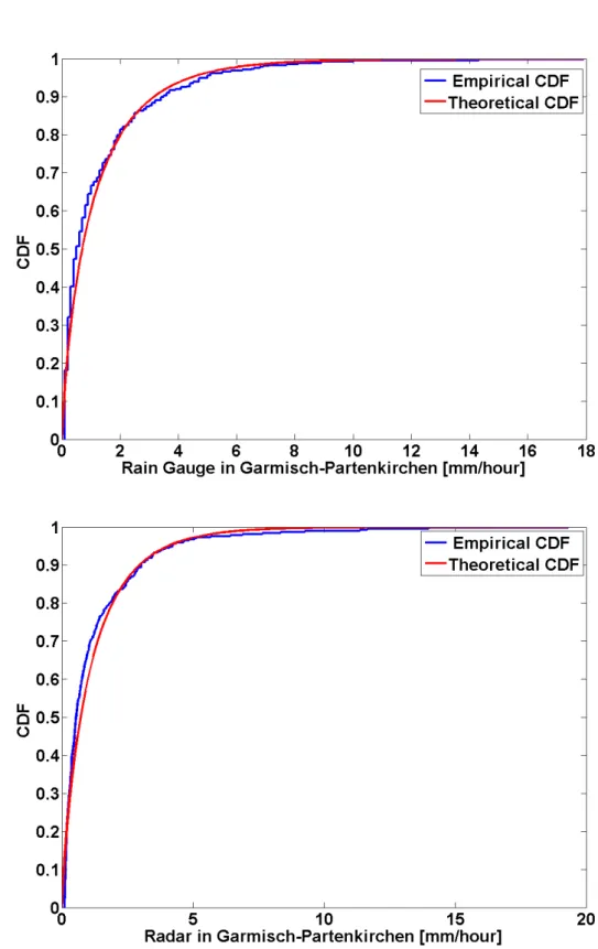
MW-link 1/gauge positive pairs as well as their marginal distributions (top to bottom), Hohenpeissenberg, June to October, 2010. . . 55 6.1 CDF of empirical and estimated theoretical marginal distribution (Weibull
distribution) for the rain gauge at Garmisch-Partenkirchen (top) and the corresponding radar grid (bottom), positive observations, summer, 2006 to 2007. . . 59 6.2 Estimated parameters of the Weibull distributions (scale/shape, top/bottom)
for radar data (positive observations) at Garmisch-Partenkirchen, Ober-ammergau and Wielenbach, in different seasons, 2005 to 2008. . . 62 6.3 Estimated parameters of the Weibull distributions (scale/shape, top/bottom)
for gauge data (positive observations) at Garmisch-Partenkirchen, Ober-ammergau and Wielenbach, in different seasons, 2005 to 2008. . . 63 6.4 Density of the empirical and estimated Gumbel Copula (from left to
right) calculated between radar/gauge positive pairs at Garmisch-Partenkirchen, summer, 2006 to 2007, w/o ARMA-GARCH transformation. . . 64 6.5 Estimated Copula parameter (Gumbel) of radar/gauge positive pairs at
Garmisch-Partenkirchen, Oberammergau and Wielenbach, in different seasons, 2005 to 2008, w/o ARMA-GARCH transformation. . . 66
LIST OF FIGURES
6.6 Time series of positive pairs of radar (Z/R-256/1.42) and gauge at Garmisch-Partenkirchen and box-plot/mean (top/bottom) of the random sample (100 realizations) of pseudo observations generated by using the Gumbel Copula, summer 2008, w/o ARMA-GARCH transformation. . . 68 6.7 Scatter plot of radar derived rainfall (blue for simple Z/R, green for
Radolan) and pseudo observations (red) at Garmisch-Partenkirchen, pos-itive pairs, summer, 2005 to 2008, w/o ARMA-GARCH transformation. 70 6.8 Density of the empirical and estimated Gumbel Copula (from left to
right) estimated between radar and gauge positive pairs at Garmisch-Partenkirchen, summer, 2006 to 2007, w/ ARMA-GARCH transformation. 71 6.9 Time series of positive pairs of radar (Z/R-256/1.42), gauge and
gener-ated pseudo observations at Garmisch-Partenkirchen, summer 2008, w/o and w/ ARMA-GARCH transformation (top/bottom). . . 73 7.1 Gumbel Copula parameterθGas a function of radius, calculated between
the gauge at Wielenbach and all the nearby radar grid cells, positive pairs only, summer, 2005 to 2008, w/o ARMA-GARCH transformation. . . . 79 7.2 Copula parameter maps showing the Copula parameter θG calculated
from the rain gauges at Garmisch-Partenkirchen, Oberammergau, Wie-lenbach and Munich (from left to right and top to bottom), summer, 2007 to 2008, w/o ARMA-GARCH transformation. The white triangle refers to the radar station at Hohenpeissenberg and the white cycle refers to Garmisch-Partenkirchen, the same all through the thesis. . . 80 7.3 Flowchart ofMultiple ThetaandMaximum Thetaapproaches for Copula
parameter map based rainfall field simulation. . . 82 7.4 Simulated field of pseudo observations derived by the Multiple Theta
approach (top) and uncorrected radar field (bottom), 13:00, 04.08.2008, Gumbel Copula, w/o ARMA-GARCH transformation. The unit of the color bar is in [mm/hour]. . . 84 7.5 Simulated fields of pseudo observations derived by the Multiple Theta
approach for a complete rainfall event from 09:00 to 16:00 (from left to right and top to bottom), 04.08.2008, Gumbel Copula, w/o ARMA-GARCH transformation. The unit of the color bar is in [mm/hour]. . . 85
7.6 Maximum theta map derived from all available Copula parameter maps, summer, 2006 to 2007, Gumbel Copula, w/o ARMA-GARCH transfor-mation. The color bar is the value of the Copula parameterθG . . . 87 7.7 Simulated field of pseudo observations derived by the Maximum Theta
approach, 13:00, 04.08.2008, Gumbel Copula, w/o ARMA-GARCH trans-formation. The unit of the color bar is in [mm/hour]. . . 88 7.8 Simulated field of pseudo observations derived by the Maximum Theta
approach for a complete rainfall event from 09:00 to 16:00 (from left to right, top to bottom), 04.08.2008, Gumbel Copula, w/o ARMA-GARCH transformation. The unit of the color bar is in [mm/hour]. . . 89 7.9 Interpolated rainfall field derived from the observed precipitation values
at 13:00, 04.08.2008. The observations from the 31 gauge stations in the radar domain were interpolated by application of an Ordinary Kriging approach. The unit of the color bar is in [mm/hour]. . . 90 7.10 Time series of radar (Z/R-256/1.42), gauges and pseudo observations
generated by using the Maximum Theta approach, positive pairs, at Garmisch-Partenkirchen, Oberammergau, Wielenbach and Munich (from left to right and top to bottom), summer, 2008, Gumbel Copula, w/o ARMA-GARCH transformation. . . 91 7.11 Copula parameter maps showing the Copula parameter θG calculated
from the rain gauges at Garmisch-Partenkirchen, Oberammergau, Wie-lenbach and Munich (from left to right and top to bottom), summer, 2007 to 2008, w/ ARMA-GARCH transformation. The color bar is the value of the Copula parameter θG. . . 94
7.12 Simulated field of pseudo observations derived by theMultiple Thetaand Maximum Theta approaches (from top to bottom), 13:00, 04.08.2008, Gumbel Copula, w/ ARMA-GARCH transformation. The unit of the color bar is in [mm/hour]. . . 95 7.13 Simulated field of pseudo observations derived by the Maximum Theta
approach for a complete rainfall event from 09:00 to 16:00 (from left to right, top to bottom), 04.08.2008, Gumbel Copula, w/ ARMA-GARCH transformation. The unit of the color bar is in [mm/hour]. . . 96
LIST OF FIGURES
7.14 Time series of radar (Z/R-256/1.42), gauges and pseudo observations generated by usingMaximum Thetaapproach, positive pairs, at Garmisch-Partenkirchen, Oberammergau, Wielenbach and Munich (from left to right and top to bottom), summer, 2008, Gumbel Copula, w/ ARMA-GARCH transformation. . . 97 8.1 The Pearson’s correlation r (top) and RMSE (bottom) calculated
be-tween the fitted and real Copula parameter θG values, by using the
polynomials under different orders forRa andz, summer, 2006 to 2007, w/o ARMA-GARCH transformation. . . 105 8.2 Copula parameter θG calculated according to Ra and z (the orders for
Ra at 4 andz at 5 in the top; the orders for Ra at 7 andz at 2 at the bottom), summer, 2006 to 2007, w/o ARMA-GARCH transformation. . 106 8.3 Copula parameterθG as a function of range and altitude (top),
interpo-lated Copula parameter θG field (middle) in summer 2006 to 2007 and
digital elevation model (bottom), w/o ARMA-GARCH transformation. The color bar is the value of the Copula parameterθG. The white
trian-gle refers to the radar station at Hohenpeissenberg and the white cycle refers to Garmisch-Partenkirchen, the same all through the thesis. . . . 109 8.4 Interpolated Copula parameter θG fields for spring, autumn and winter
(top to bottom), 2006 to 2007, w/o ARMA-GARCH transformation. The color bar is the value of the Copula parameterθG. . . 110 8.5 The Pearson’s correlation (top) and rmse (bottom) calculated between
the fitted and real Copula parameterθGvalues, by using the polynomials
under different orders forRa and z, summer, 2006 to 2007, w/ ARMA-GARCH transformation. . . 111 8.6 Copula parameterθG as a function of range and altitude (top) and the
interpolated Copula parameterθGfield (bottom), summer, 2006 to 2007,
w/ ARMA-GARCH transformation. The color bar is the value of the Copula parameter θG. . . 113
8.7 Simulated fields of pseudo observations by using the interpolated Cop-ula parameter θG field based approach, 13:00, 04.08.2008, w/o and w/ ARMA-GARCH transformation (top to bottom). The unit of the color bar is in [mm/hour]. . . 115 8.8 Simulated fields of pseudo observations by using the interpolated
Cop-ula parameter θG field based approach for a complete rainfall event from 09:00 to 16:00 (from left to right, top to bottom), 04.08.2008, w/o ARMA-GARCH transformation. The unit of the color bar is in [mm/hour].116 8.9 Simulated fields of pseudo observation the interpolated Copula
parame-ter θG field based approach for a complete rainfall event from 09:00 to
16:00 (from left to right, top to bottom), 04.08.2008, w/ ARMA-GARCH transformation. The unit of the color bar is in [mm/hour]. . . 117 8.10 Time series of pseudo observations generated by using the interpolated
Copula parameter θG field based approach, the corresponding radar
(Z/R-256/1.42) and gauge observations, for the station Garmisch-Partenkirchen, Oberammergau, Wielenbach and Munich (from left to right and top to
bottom), positive pairs, summer, 2008, w/o ARMA-GARCH transfor-mation. . . 120 8.11 Time series of pseudo observations generated by using interpolated
Cop-ula parameter θG field based approach, the corresponding radar
(Z/R-256/1.42) and gauge observations, for the station Garmisch-Partenkirchen, Oberammergau, Wielenbach and Munich (from left to right and top to bottom), summer, 2008, positive pairs only, w/ ARMA-GARCH trans-formation. . . 122 9.1 Available time period of 20 stations with both hourly precipitation and
air temperature (arranged by the station ID number in Table 9.1), 1995 to 2011. . . 128 9.2 Parameter of the estimated Exponential distribution for different
tem-peratures for all rain gauges, 1995 to 2011. . . 130 9.3 Mean precipitation intensity for different temperatures for all rain gauges,
1995 to 2011. . . 131 9.4 Linear interpolated coefficient a and b vs altitude (from top to bottom). 132
LIST OF FIGURES
9.5 Simulated field of parameter λ derived from the temperature and alti-tude driven rain gauge marginal distribution (left) and the corresponding interpolated temperature field (right), 13:00, 14.07.2008. . . 133 9.6 Scale parameter of the estimated Weibull distribution for different
tem-peratures for all rain gauges, 1995 to 2011. . . 134 9.7 Shape parameter of the estimated Weibull distribution for different
tem-peratures for all rain gauges, 1995 to 2011. . . 135 9.8 Linear interpolated coefficient ascale and bscale vs altitude (from top to
bottom), Weibull distribution. . . 136 9.9 Linear interpolated coefficientashape and bshape vs altitude (from top to
bottom), Weibull distribution. . . 137 9.10 The radar field with convective rainfall (top, highlighted as brown) and
stratiform rainfall (bottom, highlighted as brown in the first step and light green in the second step) at 13:00, 04.08.2008 . . . 139 9.11 Parameter of the estimated Exponential distribution (rain gauge) for
different different values of relative humidity (top) and both tempera-ture/relative humidity (bottom), Garmisch-Partenkirchen, positive ob-servations only, 1995 to 2011. . . 145 9.12 Estimated Copula parameterθGfor different temperatures at 6 locations
with all the radar, gauge and temperature observations in this study area, positive pairs only, 2005 to 2008, w/o ARMA-GARCH transformation. . 146 10.1 Copula parameter maps (Gumbel) derived from MW-link 1
(Hohenpeis-senberg to Weilheim, top) and MW-link 2 (from Hohenpeis(Hohenpeis-senberg to Murnau, bottom), positive pairs, June to October, 2010. The color bar is the value of the Copula parameterθG. . . 152
10.2 Pseudo observation field simulated by using Maximum Theta approach, w/o and w/ MW-link and original radar field (from top to bottom), 06:00, 04.08.2007, w/o ARMA-GARCH transformation. The unit of the color bar is in [mm/hour]. . . 155 10.3 The area (grids highlighted with red) with the Copula parameters
se-lected from the 2 MW-link derived Copula parameter maps at 06:00, 04.08.2007. . . 157
10.4 Theoretical representation of the distribution ofδi based on the the
cor-responding measurements ofRi and the MW-link L, as well as theRd. . 158
10.5 ∆ Vs δi (blue circle) and radar gauge differences (red circle) at the location of Hohenpeissernberg, July to October, 2010. . . 160 10.6 The positive time series for original and MW-link adjusted radar
mea-surements, as well as the rain gauge observation at Hohenpeissenberg, July to October, 2010. . . 161 10.7 The positive time series for original and MW-link adjusted radar
mea-surements, as well as the rain gauge observation at Wielenbach, July to October, 2010. . . 162
List of Tables
3.1 Validation measures used in this study, ( oi define the value of the
ob-servations andmi the value of the model at time step i= 1, . . . , n ). . . 23
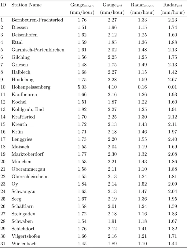
4.1 The description of available rain gauge stations and air temperature observations in this study area, both in hourly. . . 28 4.2 Technical descriptions of C-band weather radar at Hohenpeissenberg . . 31 4.3 Mean and standard deviation for gauge and radar (positive pairs only)
in the period of June, July, and August, 2006 to 2007. . . 34 4.4 The probabilities -p00, p01, p10andp11- for each group of the locations at
Garmisch-Partenkirchen, Oberammergau, Wielenbach and Munich City in different seasons from 2005 to 2008. . . 35 4.5 PCA coefficients for air temperature T, ∆T, relative humidity, ∆RH,
mean wind speed and ∆M W S at Garmisch-Partenkirchen for (0,0), (1,0), (0,1) and (1,1) cases in different seasons from 2005 to 2008. . . 36 4.6 Ljung-Box Q-test for radar and gauge (positive pairs only) and their
residuals after performing ARMA-GARCH transformation, under dif-ferent lags, for selected rain gauge stations at Garmisch-Partenkirchen, Oberammergau and Wielenbach (June, July, and August of 2006 to 2007), alpha = 0.01, 1 means autocorrelated, 0 means no autocorrelation. 37 4.7 Ljung-Box Q-test for radar and gauge (positive pairs only) and their
residuals after performing ARMA-GARCH, under different lags, for se-lected rain gauge stations at Garmisch-Partenkirchen, Oberammergau and Wielenbach (June, July, and August of 2006 to 2007), alpha = 0.05, 1 means autocorrelated, 0 means no autocorrelation. . . 40
4.8 Engle test for radar and gauge (positive pairs only) and their residuals after performing ARMA-GARCH transformation, under different lags, for selected rain gauge stations at Garmisch-Partenkirchen, Oberam-mergau and Wielenbach (June, July, and August of 2006 to 2007), alpha = 0.01, 1 means conditional heteroscedasticity, 0 means no conditional heteroscedasticity. . . 41 4.9 Engle test for radar and gauge (positive pairs only) and their residuals
after performing ARMA-GARCH transformation, under different lags, for selected rain gauge stations at Garmisch-Partenkirchen, Oberam-mergau and Wielenbach (June, July, and August of 2006 to 2007), alpha = 0.05, 1 means conditional heteroscedasticity, 0 means no conditional heteroscedasticity. . . 42 5.1 The geographical and technical description of the 2 MW-links . . . 52 6.1 AIC and BIC calculated for rain gauges and the corresponding radar
measurements (positive observations, ≥0.1 [mm/hour]) for selected lo-cations at Garmisch-Partenkirchen, Oberammergau and Wielenbach, for different univariate theoretical distribution functions, summer, 2006 to 2007. . . 60 6.2 Goodness of Fit (GoF) test using the K-function. The minimum values
of the K function value are highlighted in bold, suggesting the best fit, summer, 2006 to 2007, w/o ARMA-GARCH transformation. . . 65 6.3 Comparison of the rainfall calculated with the simple Z/R (256/1.42)
relationship, Radolan derived rainfall, Copula-based pseudo observations (both data and rank space) and rain gauges at Garmisch-Partenkirchen, Oberammergau, Wielenbach and Munich City, only for positive pairs, summer, 2005 to 2008, w/o ARMA-GARCH transformation. The best ones are highlighted in bold. . . 67 6.4 Goodness of Fit (GoF) test using the K-function. The minimum values
of the K function value are highlighted in bold, summer, 2006 to 2007, w/ ARMA-GARCH transformation. . . 71
LIST OF TABLES
6.5 Validation for Copula-based simulated pseudo observations for all sta-tions, positive pairs only, summer, 2008, w/o ARMA-GARCH transfor-mation. . . 74 6.6 Validation for Copula-based simulated pseudo observations for all
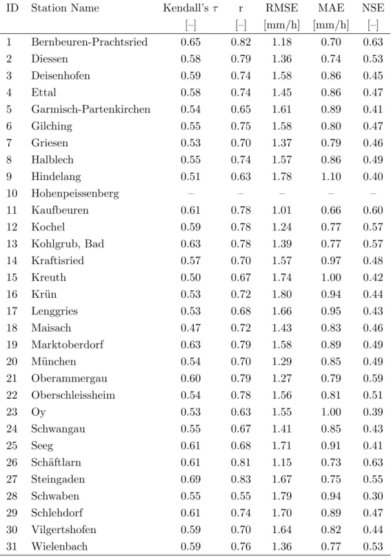
sta-tions, positive pairs only, summer, 2008, w/ ARMA-GARCH transfor-mation. . . 75 7.1 Point wise cross-validation for theMultiple Theta approach during 2008
summer, for all stations, positive pairs only, Gumbel Copula, w/o ARMA-GARCH transformation. . . 92 7.2 Point wise cross-validation for Maximum Theta approach during 2008
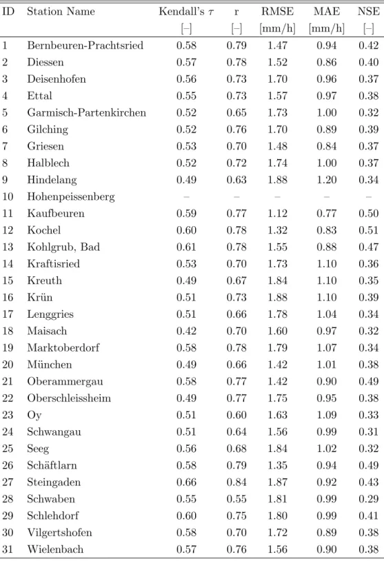
summer, for all stations, positive pairs only, Gumbel Copula, w/o ARMA-GARCH transformation. . . 93 7.3 Point wise cross-validation of the Multiple Theta and Maximum Theta
approach for all stations, summer 2008, positive pairs only, Gumbel Cop-ula, w/ ARMA-GARCH transformation. . . 98 8.1 Coefficients of the fitted two variates polynomial, summer, 2006 to 2007,
w/o ARMA-GARCH transformation. . . 107 8.2 Residuals between between the fitted and real Copula θG values
(ar-ranged by the number in Table 4.1, ID number 10 of Hohenpeissenberg is not included), summer, 2006 to 2007, w/o ARMA-GARCH transfor-mation. . . 107 8.3 Coefficients of the fitted bivariate polynomial, summer, 2006 to 2007, w/
ARMA-GARCH transformation. . . 112 8.4 Residuals between between the fitted and real CopulaθGvalue (arranged
by the number in Table 4.1, ID number 10 of Hohenpeissenberg is not included), w/ ARMA-GARCH transformation. . . 114 8.5 Point wise cross-validation for interpolated Copula parameter θG field
based approach for all the stations, summer, 2008, positive pairs only, w/o ARMA-GARCH transformation. . . 119 8.6 Point wise cross-validation for interpolated Copula parameter θG field
based approach for all stations, summer, 2008, positive pairs only, w/ ARMA-GARCH transformation. . . 121
9.1 Description of the 20 stations with both hourly precipitation and air temperature observations, 1995 to 2011, Bavaria, Germany . . . 127 9.2 Comparison of marginal distributions for gauge/radar (parameter λ of
Exponential distribution), and Copula parameter (θG) estimated in con-vective and stratiform rainfall types for Garmisch-Partenkirchen, Ober-ammergau, Wielenbach and Munich, positive pairs, summer, 2006 to 2007, w/o ARMA-GARCH transformation. . . 140 9.3 Pearson’s correlation coefficient calculated between rain gauge
observa-tions and generated pseudo observaobserva-tions from different combination of spatial distribution for the dependence structure and gauge marginal distributions, positive pairs only, summer, 2008, w/o ARMA-GARCH transformation. . . 142 9.4 RMSE [mm/hour] calculated between rain gauge observations and
gen-erated pseudo observations from different combination of spatial distri-bution for the dependence structure and gauge marginal distridistri-butions, positive pairs only, summer, 2008, w/o ARMA-GARCH transformation. 142 9.5 NSE calculated between rain gauge observations and generated pseudo
observations from different combination of spatial distribution for the dependence structure and gauge marginal distributions, positive pairs only, summer, 2008, w/o ARMA-GARCH transformation. . . 143 10.1 Point wise cross-validation for MW-link included Maximum Theta
ap-proach in different stations, summer, 2008, w/o ARMA-GARCH trans-formation. . . 156
Glossary
AIC Akaike Information Criterion BIC Bayesian Information Criterion CDF Cumulative Distribution Function CPM Copula Parameter Map
CSMD Convective and Stratiform dependent Marginal Distribution DEM Digital Elevation Model
DWD Deutscher Wetterdienst or German Weather Service DSD Drop Size Distribution
FMD Fixed Marginal Distribution GoF Goodness of Fit
ICPF Interpolated Copula Parameter Field IDW Inverse Distance Weighted
i.i.d. Independent and Identically Distributed MAE Mean Absolute Error
MD Marginal Distribution
MLE Maximum Likelihood Estimation
MOHP Meteorological Observatory Hohenpeissenberg MW-link Microwave Link
NaN Not A Number
NSE Nash-Sutcliffe Efficiency UTC Coordinated Universal Time PCA Principle Component Analysis PDF Probability Density Function r Pearson’s Correlation Coefficient RMSE Root Mean Square Error
TAMD Temperature and Altitude driven Marginal Distribution
w/ With
A Attenuation
Ar The elective aperture (area) of the receiving antenna R Radar derived rainfall
Ra Range
F Pattern propagation factor
G Gauge derived rainfall
Gt The gain of the transmitting antenna
L MW-link derived rainfall
M W S Mean wind speed
o Observation values
P Precipitation
Pt The transmitter power of radar RH Relative humidity
T Temperature
Z Radar reflectivity
z Altitude
θF Frank Copula parameter θG Gumbel Copula parameter θC Clayton Copula parameter
σ The radar cross section, or scattering coefficient, of the target
1
Introduction
1.1
Motivation
Sustainable water management has become an issue of major concern over the past decades (e.g. Pahl-Wost et al., 2007). The importance of water resources and manage-ment has also be highlighted in recent climate studies with respect to political decision making and risk analyses (e.g. IPCC, 2007; IPCC, 2008). Increasing water demands in agriculture, industry and households lead to the declining fresh water availability which restricts economic development and wealth particular in water scarce environ-ments with weak or vulnerable infrastructures (e.g. Orr et al., 2009). Understanding the hydrological cycle is fundamental to investigate all things related to water, which is also a key to the proper management of water resources. Precipitation is the principle source of the Earth’s water supply so that the spatio-temporal distribution of rainfall is an important aspect within hydrological processes (e.g. Kuchment et al., 2004).
Traditional rain gauges are good point local observation tools but limited to their low spatial representativeness. In contrast, weather radar reflectivity measurements can provide spatial pattern information. However, the transformation of reflectivity to rain rate is accompanied by tremendous uncertainties (e.g. Habib et al., 2008; Villarini et al., 2008). The differences between radar and rain gauge observations can amount to 100 percent or even more due to random and systematic errors as e.g. reported by Smith et al. (1996). The discrepancies between rain gauges and the corresponding radar measurements are mainly due to the different spatio-temporal sampling properties. Rain gauges measure ground precipitation only at one point in space, while radar
measures indirect volumetric rainfall aloft in the atmosphere depending on the radar elevation angle and range from the radar station (e.g. Ehret et al., 2002).
These traditional rainfall measurement techniques inspired the use of microwave link attenuation, which has been proven to provide accurate line integral rainfall ob-servations at the near-surface level (e.g. Messer et al., 2006; Leijnse et al., 2008). Comparing to gauge and radar, the installation of MW-links designating for rainfall monitoring is costly and not complicated. Furthermore, it is also feasible to use of MW-link attenuation data from commercial cellular network operators for monitoring rainfall fields (e.g. Giuli et al., 1991, 1999, and 2007; Zinevich et al., 2008).
So, the challenge lies on how to assimilate the precipitation information from differ-ent observation devices, such as rain gauge, radar and MW-link. As the distribution of precipitation is usually non-Gaussian, Copula-based approaches are applied to assimi-late data from rain gauge and MW-link to radar precipitation fields simultaneously by the studying the dependence structures among them.
1.2
State of the Art
Traditionally, without the spatial precipitation information from remote sensing tech-niques, the rain gauge observations alone were used to derive the precipitation fields by using various interpolation methods. Among them, nearest neighbour (e.g. Isaaks et al., 1989), inverse distance weighting, regression models (e.g. Bourrough and Mc-Donell, 1998), trend surface analyses (e.g. Colins and Bolstadt, 1996) and Splines (e.g. Hutchinson et al., 1998a and 1998b; Bourrough and McDonell, 1998) are some exam-ples, as well as the Kriging approach with a large set of sub-methods developed (e.g. Isaaks et al., 1989; Bollerlslev et al., 1986; Goovaerts et al., 2000; Haberlandt et al., 2007). The mixture use of different methods can also been found such as regression combined with Kriging (e.g. Erxleben et al., 2002). All those methods are different from each other in nature. However, they share with the common problems that: their performance is highly dependent on the density of the observation network (e.g. DWD, 2000) and the complexity of the underlying terrain has directly impacts on the pre-cipitation (e.g. Kyriakidis et al., 2001; Roe et al., 2005). Especially in regions with complex terrain and very large altitude gradients, very few or even no meteorological stations providing reliable rainfall measurements can be available.
1.2 State of the Art
In recent years, with the development of radar technology, precipitation fields from weather radar are widely used and supposed to be a good supplement with the abil-ity to cover areas with complex terrain in fine spatio-temporal resolutions so that the patterns of rainfall are realistically reproduced (e.g. DWD, 2000; Vogl et al., 2012). However, multiple sources of errors exist in the precipitation fields derived from radar reflectivities, such as the empirical reflectivity/rainfall (Z/R) relationship, errors in-duced by the radar measurement itself such as backscatter or shadowing effects (e.g. Joss and Lee, 1995; Vogl et al., 2012) and etc.. When radar fields are used as the in-puts to drive meteorological or hydrological models, these errors have to be taken into account carefully (e.g. Cole and Moore, 2008; Singh et al., 1997) as they will directly be propagated and can increase the uncertainty of the predicted variables.
As a result, it is straightforward and logical to join the advantages of both measure-ment devices, the point accurate rain gauge and spatial superior radar fields. In the past, many methods have been developed to jointly use both data sources combining their advantages, from simple to very sophisticated ones. They can be roughly clas-sified into following different classes: gauge adjusted radar, geo-statistical approaches and the other methods (especially for Copula-based approaches in this study).
The first group was trying to reduce the uncertainties in the radar derived precipi-tation fields by using information from gauge. This can be done by improving the radar Z/R relationship by using rain gauge measurements (e.g. Brandes et al., 1975; Marx et al., 2007; DWD, 2000 and 2001) to correct for errors in the radar absolute values. However, the Z/R relationship is strictly dependent on the rainfall type and can have high spatial variations even in one event because of the topography and etc.. Another way is the multiple adjustment (e.g. Collier et al., 1986; Moore et al., 1994b; DWD, 1998) by calculating gauge based correction factor to modify the radar fields, trying to reduce the mean field bias or the other means (e.g. Erxleben et al., 2002). Although this kind of approach can provide satisfying results in certain specific test regions, the assumption behind is simple. The applications of these methods are all dependent on the density of rain gauge network and therefore their performances are limited in the data sparse regions.
The second way is the geo-statistical methods developed to account for the dif-ferent sampling properties of radar and rain gauge, especially for the Kriging based approaches. The so called Co-Kriging was developed to combine radar and gauge data
(e.g. Krajewski et al., 1987), with the assumptions that the rainfall field is second order stationary, random errors for the rain gauges, uncorrelated in time with zero mean and etc.. Alternatively, in the work e.g. done by Seo et al. (1990a and 1990b), Univer-sal Kriging was used to combine radar and gauge data. Furthermore, by using both gauge data and digital elevation model, Goovaerts et al. (1999) developed an extensive cross-validation comparison of different rainfall interpolation techniques. However, so-phisticated Kriging with the additional complexity did not pay off in the form of better results compared to simpler Kriging techniques (e.g. Ehret et al., 2002). Furthermore, the crucial problem is that the distribution of precipitation is assumed to be Gaussian or alternative versions of Gaussian in those traditional approaches.
However, the hydro-meteorological variables are usually non-Gaussian (e.g. AghaK-ouchak et al., 2010b) and also require bi or multivariate analyses as well as conditional probability distributions of variables (e.g. Genest and Favre, 2007) The Copula-based approach, with the ability to capture non-linear behaviour, is not limited to the Gaus-sian distribution (e.g. Nelson et al., 1999). Over the past decades, there is a remarkable increase in applications of Copulas in hydro-meteorology. Alternatively, the Copulas were used to describe the complex spatio-temporal dependence structure and assess for non-linear behaviour (e.g. Genest and Favre, 2007; Dupois et al., 2007). The Cop-ula based methods are advantageous in many respects and have already been used successfully in risk assessment (e.g. Frees and Valdez, 1998).
Roughly about 10 years ago, the Copulas started its application in the field of hydro-meteorology. Recently a remarkable increase in the Copulas related publications can be found for multivariate frequency analyses, geo-statistical interpolation and multivariate extreme value analyses (e.g. Michele and Salvadori, 2003; Dupois et al., 2007; B´ardossy et al., 2006; Genest and Favre, 2007; Renard and Lang, 2007; Schoelzel and Friederichs, 2008; B´ardossy and Li, 2008; Zhang and Singh, 2008). Considering about precipita-tion field, in the work done by Michele and Salvadori (2003), Copulas were used to model intensity-duration of rainfall events. Favre et al. (2004) developed Copula-based approach for multivariate hydrological frequency analysis, and then, Zhang and Singh (2008) utilised the Archimedean Copulas to perform the bivariate rainfall frequency analyses. Renard and Lang (2007) investigated the usefulness of the Gaussian Copula in extreme value analyses and Kuhn et al. (2007) tried to describe spatial and temporal dependence of weekly precipitation extremes by using the Copula-based approach. In
1.2 State of the Art
the work by Serinaldi et al. (2008), the author suggested a Copula-based mixed model for modelling the dependence structure and the corresponding marginal distributions, which is based on the properties of the non parametric Kendall’s rank correlation and the upper tail dependence coefficient calculated from the dependence structure between pair wise observations from different rain gauges. Recently, Copula-based models were developed for the purpose to estimate the point scale or spatial distribution of errors in the radar derived precipitation fields (e.g. Villarini et al., 2008; AghaKouchak et al., 2010a and 2010b).
However, in most of these studies, the dependence structure is calculated between two variates in the bivariate framework, only with few examples of multivariate appli-cations. B´ardossy developed a new Copula-based geo-statistical interpolation method (e.g. B´ardossy et al., 2006; B´ardossy and Li, 2008; B´ardossy and Pegram, 2009), especially the new Copula family named v-transformed Copulas. In their work, the multivariate Copulas were used to describe the spatial variability of environmental vari-ables, e.g. groundwater quality parameters. Then a methodology was also proposed to perform the spatially interpolation for these quantities and the gauge observed daily precipitation.
Recently, the new remote sensing techniques, such as dual microwave links (e.g. Holt et al., 2003; Rahimi et al., 2004; Minda et al., 2005; Leijnse et al., 2007a) and wireless communication networks (e.g. Messer et al., 2006), show to be good comple-mentaries to gauge and radar. The estimation of spatial rainfall fields based on the microwave link attenuation was proposed in the work as e.g. done by Giuli et al. (1991, 1999 and 2007) and Zinevich et al. (2008), also with the effort to adjust radar field by using MW-link derived rainfall (e.g. Cummings and Upton, 1996). Even though some uncertainties are still associated with their application to derive precipitation infor-mation, the widely applications of MW-link attenuation are very promising, not only due to the network of observations especially in the mountain areas but also because of very low costs comparing to gauge and radar, nearly free for commercial wireless communication networks (e.g. Messer et al., 2006).
1.3
Objectives
This study aims to develop stochastic approaches for estimating precipitation fields through assimilating data from various rainfall observation devices. Especially in the region with complex terrain, there are limited numbers of observation tools such as rain gauges. Usually, large differences are found here between precipitation fields derived from different devices. So, it is necessary and also the main objective to estimate the precipitation fields combing the advantages from different measurement tools.
Considering the point accurate rain gauge and spatial priority radar, the Copula-based analysis is chosen and capable to combine the advantages from both sides by investigating the dependence structures between them. As a result, the overall objec-tives of this study are:
1. Revealing the spatial distribution of dependence structures between rain gauge and radar.
2. Deriving the spatial distribution of marginal distribution for rain gauges.
3. Investigating the sensitivity of ARMA-GARCH transformation to the simulated precipitation fields.
4. Improving the estimated precipitation fields by including the precipitation infor-mation further from MW-Links.
1.4
Structure of the Dissertation
With respect to the scope of this study, the thesis is divided into 11 chapters. After the introduction and innovation, in the 3rd chapter, an overview on Copulas theory is presented, as well as the Copula-based simulation techniques and validation methods. In Chapter 4, traditional data sources (radar and gauge) and their data pre-processing are briefly introduced, including the demonstration why the gauge can be used to determine the wet/dry periods and the assumption of independent and identically dis-tributed (i.i.d.). In the 5th chapter, the physical background of MW-link is introduced, followed by the comparisons between MW-link derive precipitation and gauge/radar. In Chapter 6, the point wise assimilation to combine precipitation information from rain gauge and radar is introduced and the impacts from ARMA-GARCH transformation
1.4 Structure of the Dissertation
are investigated. Afterwards, two Copula-based spatial data assimilation approaches are proposed, which are the Copula parameter map based method in Chapter 7 and interpolated Copula parameter field based algorithm in Chapter 8. The impacts from ARMA-GARCH transformation are also investigated in the spatial case. In the 9th chapter, several spatial distributions of rain gauge marginal distributions are developed, and then the simulation results from combinations of different spatial dependence struc-tures and gauge marginal distributions are presented and compared. The precipitation derived from MW-links is integrated to further improve the estimated rainfall fields in the 10th chapter. The final chapter is devoted to summary and conclusions and recommendations for further research.
2
Innovation
Innovative work of this thesis includes:
1. Applying Copula analysis on the hourly precipitation observations, beyond the limitation of Gaussian assumption implied in the traditional geo-statistical ap-proaches.
2. Establishing the Copula parameter map and interpolated Copula parameter field based approaches to simulate precipitation fields of pseudo observation assimi-lating observations from gauge and radar, with a superior performance and also very low computational costs.
3. Developing the spatial distribution of marginal distributions for rain gauges driven by the temperature and altitude.
4. Performing ARMA-GARCH transformation to remove autocorrelation and het-eroskedasticity and also investigating the sensitivity of ARMA-GARCH transfor-mation to the final precipitation fields.
5. Including MW-link attenuation as an independent and complementary precipi-tation observation tool to further constrain and improve the precipiprecipi-tation fields derived from gauge and radar.
3
Review of Copula Theory
3.1
Introduction
The definition of Copulas first appeared in 1959 in the work of Sklar et al. (1959), which are used to model the dependence structure between two or more variables. The term of Copulas originally derived from Copulare, a Latin word which means to join, connect or link. The use of Copulas makes it possible to calculate bivariate or multi-variate distributions of random variables with great flexibility. Traditional bimulti-variate or multivariate distribution families, such as bivariate normal, log-normal and gamma, are built with a number of model parameters that describe the behaviour of each random variable as well as the joint probability distribution itself (e.g. AghaKouchak et al., 2010b). The main disadvantage of those approaches is that modelling the dependence structure between variables is not independent of the choice of the marginal distribu-tions (e.g. Genest and Favre, 2007). However, the Copula based approaches allow to avoid this restriction and also not limited by the Gaussian assumption. Furthermore, by using the Copulas, the dependence structure keeps the same after performing any monotonic increasing transformations on the variables. As already described in section 1.2, the application of Copulas, in multivariate simulation, extreme value analysis and modelling of the dependence structure have become popular in the field of hydrology and meteorology.
In section 3.2, the theoretical background of Copula theory is given. Afterwards the Copula families used in this study are described in section 3.3, followed by the introduction of marginal distribution in section 3.4. Then the advantages of Copulas
are summarized in section 3.5. Finally, the algorithm for Copula-based simulation of pseudo observations is explained step by step in section 3.6.
3.2
Copula Theory
The Copula theory is briefly introduced in this section. First, Sklar’s theorem is ex-plained, followed by the bounds and properties for Copulas. The method to build empirical Copula is described and several important concepts and definitions are given, such as Kendall’s τ Spearman’s ρ and upper/lower tail dependence coefficients. More detailed information about Copula theory can be found e.g. in Joe et al. (1997); Frees and Valdez (1998); Nelson et al. (1999); Salvadori et al. (2007).
3.2.1 Sklar’s Theorem
Considering a vector random variable,X = [X1, ..., Xn]
0
, with joint distributionF(x1, ..., xn)
and marginal distributionsFXi(xi), according to the theorem developed by Sklar et al.
(1959), the multivariate distribution F can be expressed in terms of a Copula C and the corresponding marginal distributions:
F(x1, ..., xn) =C(FX1(x1), . . . , FXn(xn)), (3.1)
The n-dimensional Copulas are functions defined as listed in Eq. (3.2), linking univariate distribution functions together to form a multivariate distribution function.
C: [0,1]n→[0,1]. (3.2) As for general distribution functions, the density of a Copula C(u, v), here u =
FX1(x1) andv=FX2(x2), is calculated as
c(u, v) = ∂
2C(u, v)
∂u∂v . (3.3)
Therefore, the probability density (PDF) of the multivariate distributionf(x1, ..., xn),
can be expressed in terms of a Copula PDFcand PDF of marginal distributionsfXi(xi).
So the Copula PDFc is often called the dependence function.
3.2 Copula Theory
With the ability to link multivariate distributions to their marginals, Copulas also allow to merge the dependence structure from the marginal distributions to form their joint multivariate distribution. The Copula function is unique when the marginals are steady functions. As the Copula is only a reflection of the dependency structure itself, their construction is reduced to the study of the relationship between the correlated variables, giving freedom for the choice of the univariate marginal distributions. This is the main advantage of Copula-based approaches.
3.2.2 The Frechet-Hoeffding Bounds for Copulas
The Frechet-Hoeffding bounds describe the upper and lower bounds for every Copula with u and v elements (the bivariate cases are taken an example in this Chapter and can be easily extended to multivariate cases). These bounds are described by
max(u+v−1,0)≤C(u, v)≤min(u, v) (3.5) where, W(u, v) = max(u +v −1,0) is the lower bound and the upper bound is given by M(u, v) = min(u, v). It should be noted that W(u, v) and M(u, v) are Copulas themselves.
3.2.3 Properties of Copulas
The Copula approach allows to account for the fact that the dependence structure between two variates (u=FX(x), v =FY(y)) is more complex than it can be modelled by the multivariate normal distribution or ordinary dependency measures such as e.g. the Pearson correlation coefficient. Another important property of Copula functions is the fact that they are invariant under increasing monotonic transformations. In practice, it means that data may be transformed (e.g. by taking the logarithm or de-trending) without changing its Copula. The other general properties of Copulas as e.g. given by Genest and Rivest (1993) are:
1. In the bivariate case, a Copula is defined as a function C from [0,1]2 to [0,1] so that∀u, v∈[0,1] :
C(u,0) = 0 =C(0, v) (3.6)
2. A Copula is 2-increasing means that ∀u1, u2, v1, v2 ∈ [0,1] with u1 ≤ u2 and
v1≤v2 holds
C(u2, v2)−C(u2, v1)−C(u1, v2)−C(u1, v1)≥0. (3.8)
3. A Copula is continuous. Thereby satisfying the stronger Lipschitz condition. |C(u2, v2)−C(u2, v1)| ≤ |u2−u1|+|v2−v1|. (3.9)
4. A Copula has a survival Copula, C, given by
C(u, v) = 1−u−v+C(1−u,1−v) (3.10) And the joint survival function, C, for two uniform random variables (0,1), is:
C(u, v) =P[U > u, V > v] = 1−u−v+C(u, v) =C(1−u,1−v) (3.11) Therefore,
C(u, v) =C(1−u,1−v) (3.12) 3.2.4 Empirical Copulas
The empirical CopulaCn(u, v), which is defined on the rank space (or the corresponding
CDF values), is an estimator for the unknown theoretical Copula distributionCθ(u, v)
associated with the pair (X, Y) having a set of parametersθ (e.g. Genest and Rivest, 1993; Laux et al., 2011): Cn(u, v) = 1/n n X i=1 1 ri n+ 16u, si n+ 16v (3.13) where (r1, s1), . . . ,(rn, sn) denote the pairs of ranks of the data (x1, y1), . . .(xn, yn), and
1(. . .) is the indicator function.
3.2.5 Kendall’s τ and Spearman’s ρ
There is a functional relationship between the classical dependence parameters such as Kendall’s τ and Spearman’s ρ (e.g. Genest and Rivest, 1993; Laux et al., 2011).
ρ= 12 Z [0,1]2 u v dCθ(u, v)−3 = 12 Z [0,1]2 Cθ(u, v)dudv−3 (3.14) and τ = 4 Z [0,1]2 Cθ(u, v)dCθ(u, v)−1 (3.15)
3.3 Copula Families
3.2.6 Upper/Lower Tail Dependence
Tail dependence relates the amount of dependence in the upper-right-quadrant tail or in the lower-left-quadrant tail for a bivariate distribution. The upper and lower tail dependence parameters of the random vector (X, Y) with CopulaC, can be defined in the following way (e.g. Joe et al., 1997):
λup≡ lim u→1−P(Y > F −1 Y (u)|X > F −1 X (u)) = lim u→1− 1−2u+C(u, u) 1−u (3.16) and λlow ≡ lim u→0+P(Y ≤F −1 Y (u)|X ≤F −1 X (u)) = lim u→0+ C(u, u) u (3.17)
The upper tail dependence expresses the probability occurrence of positive large values (outliers) at multiple locations jointly while the lower tail dependence expresses the the probability occurrence of positive small values.
3.3
Copula Families
The two most commonly used Copula families are the Elliptical and the Archimedean Copula families. These Copulas are called Elliptical because they can be constructed from elliptical distributions. Since this Copula family closely related to the multivariate normal distribution, it provides important examples of multivariate distributions. How-ever, the Elliptical Copula shows a symmetrical upper/lower tail dependence structure so that the application of this Copula family is limited.
Archimedian Copulas are defined as following, letϕ: [0,1]→[0,∞] a steady, strict monotonic function with ϕ(1) = 0 and let ϕ[−1] : [0,∞]→[0,1] the pseudo-inverse of
ϕ(e.g. Nelson et al., 1999):
ϕ[−1] :=
ϕ−1(t) if 0≤t≤ϕ(0),
0 else (3.18)
then the function
C: [0,1]2 → [0,1]
(u, v) 7→ ϕ[−1](ϕ(u) +ϕ(v)) (3.19) defines a Copula only ifϕ is convex and ϕis called the generator of the Archimedian CopulaC.
3.3.1 Gaussian Copula
The Gaussian Copula is derived from the multivariate normal distribution ϕR. The
CDF of the Gaussian Copula is defined as:
C(u, v) =ϕR(φ−1(u), φ−1(v)) (3.20)
WhereR is the linear correlation matrix and φ−1 is the inverse of the univariate stan-dard normal distribution function. Note that the equation above is for the bivariate case; for the multivariate case, equation can be written as
C(u1,· · ·, un) =ϕR(φ−1(u1),· · ·, φ−1(un)) (3.21)
If the marginal distributionsu1=F1(x1),· · ·, un=Fn(xn) are normal, then the random
vector (x1, , xn) has a multivariate normal distribution.
3.3.2 Student-T Copula
The Student-T Copula is derived from the multivariate t-distribution. The CDF of the Student-T Copula can is defined as:
CΘ(u, v) =tν,Σ(tν−1(u), t−ν1(v)) (3.22)
Θ = {(ν,Σ) :ν ∈ (1,∞),Σ ∈ <m×m}, t
ν is a univariate t distribution withν degrees
of freedom and tν,Σ is the multivariate tdistribution with a correlation matrix Σ with
ν degrees of freedom
3.3.3 Gumbel Copula
The CDF of the Gumbel Copula is defined as
Cθ(u, v) =e−((−ln(u)θ)+(−ln(v)θ))
1
θ
(3.23) with θ >1. It is an Archimedean Copula with the generator ϕ(t) = (−ln(t))θ. This Copula is usually used for asymmetrical tail dependence structure (e.g. Nelson et al., 1999).
3.4 Marginal Distributions
3.3.4 Clayton Copula The Clayton Copula is defined as
Cθ(u, v) = u−θ+v−θ−1− 1 θ (3.24) whereθ >0. It is also an Archimedean Copula with the generator ϕ(t) = 1θ t−θ−1. The Clayton Copula is known to be asymmetrical and has a lower tail dependency 3.3.5 Frank Copula
The Frank Copula is defined as
Cθ(u, v) =−1 θln 1 +(e −θu−1)(e−θv −1) e−θ−1 (3.25) withθ >0. It is also an Archimedean Copula with the generatorϕ(t) =−ln
e−θt−1 e−θ−1
Note that as θ → 0 the dependence becomes maximal and for θ = 1 independence is achieved. This Copula is known to be symmetrical.
3.4
Marginal Distributions
Generally, e.g. for a bivariate joint distribution of (X, Y), the marginal distribution of X is calculated by summing or integrating the joint probability distribution over
Y, and the same for Y. For discrete random variables, the marginal probability mass function can be written as P r(X=x). This is
P r(X=x) =X
y
P r(X=x, Y =y) =X
y
P r(X=x|Y =y)P r(Y =y) (3.26)
whereP r(X=x, Y =y) is the joint distribution ofX andY, whileP r(X =x|Y =
y) is the conditional distribution of X givenY.
Similarly for continuous random variables, the marginal probability density function can be written aspX(x). This is
pX(x) = Z y pX,Y(x, y)dy= Z y pX|Y(x|y)pY(y)dy (3.27)
where px,y(x, y) gives the joint distribution of X and Y, whilepX|Y(x|y) gives the
conditional distribution for X given Y. Again, the variable Y has been marginalized out.
In this study, 4 different theoretical distribution functions are tested to find the best fit and their formulas are listed below.
1. The Normal distribution with meanµ and standard deviationσ f(x) := √1 2πσe −1 2( x−µ σ ) (3.28)
2. The Exponential distribution with parameter λ∈R>0
fλ(x) :=
λe−λx if x≥0,
0 else (3.29)
3. The Weibull distribution withα >0,β >0 and if β = 1, the Weibull reduces to Exponential.
f(x) :=αβxβ−1e−αxβ (3.30) 4. The Gamma distribution withb, p∈Rand b >0,p >0, where Γ(p) denotes the
value of the Gamma function atp
fλ(x) := ( bp Γ(p)x p−1e−bx if x≥0, 0 else (3.31)
All the marginal distributions of the positive rainfall amounts were estimated by maximum likelihood for each gauges, radar or MW-links at each location/grid. The distribution was chosen with the minimum value of the Akaike Information Criterion (AIC) value, which is a measure of the relative Goodness of Fit of a statistical model developed by Akaike et al. (1974). The Bayesian information criterion (BIC) is an updated version of AIC considering the number of data. The AIC and BIC are defined as:
AIC = 2k−2 ln(L) (3.32) and
BIC =kln(n)−2 ln(L) (3.33) where k is the number of parameters in the statistical model, n is the number of data in x and L is the maximized value of the likelihood function for the estimated model.
3.5 ARMA-GARCH Transformation
3.5
ARMA-GARCH Transformation
The algorithm for ARMA-GARCH transformation taken from Laux et al. (2011) and the detail information can be e.g. found in Engle et al. (1982) and Bollerlslev et al. (1986).
This section describes the theory of the ARMA-GARCH composite model to pro-duce independent and identically distributed i.i.d. residuals. An ARMA model is used to compensate for autocorrelation, and a GARCH model to compensate for the heteroskedasticity.
The GARCH − Generalized Autoregressive Conditional Heteroskedasticity is a time series modelling technique that includes past variances for predicting present or future variances. A univariate model of an observed time series ytcan be written as
yt=E(yt|Ωt−1) +εt (3.34)
In this equation, the termE(|) denotes the conditional expectation operator, Ωt−1
the information set at time t−1, and εt the innovations at time t. Bollerlslev et al. (1986) developed GARCH as a generalization of the ARCH volatility modelling technique (Engle et al., 1982). The distribution of the residuals, conditional on the timet, is given by V art−1(yt) =Et−1(ε2t) =σ2t (3.35) where σt2=κ+ X i=1,P Giσt2−i+ X i=1,Q Aiε2t−j (3.36)
where κ is a constant, and σt2 is the prediction of the variance, given the past se-quence of variance predictions σt2−i, and past realizations of the variance itself ε2t−j. When P = 0, the GARCH (0, Q) model becomes the original ARCH(Q) model in-troduced by Engle et al. (1982). This equation mimics the variance clustering of the variable (i.e. precipitation). The lag lengths P and Q and the coefficients Gi and Aj
determine the degree of persistence.
A common assumption is that the innovations are serially independent, however, GARCH(P, Q) innovations, εt, are modelled as
t is the conditional standard deviation given by the square root of Eq. (3.35), and
Ztis the standardizedi.i.d.. random draw from some specified probability distribution. Usually, a Gaussian distribution is assumed such thatε∼N(0, σt2). Reflecting this, Eq. (3.36) illustrates that a GARCH innovations processεt simply rescales ani.i.d process Zt such that the conditional standard deviation incorporates the serial dependence of
Eq. (3.35).
3.6
Copula-Based Analysis and Simulation
In this section, the Copula-based analysis and simulation techniques are introduced. First is the Goodness of Fit (GoF) test to choose the best theoretical Copula function to model the dependence structure derived from the empirical Copulas. In the second section, the Copula-based simulation techniques are described in detail. Finally, the validation measures are presented, which are used in this study to check the quality of the simulations.
3.6.1 Goodness of Fit Tests
Goodness of Fit tests for Copulas are applied by comparing the empirical Copula Cn
with the parametric estimate of a theoretical Copula modelCθ derived under the null
hypothesis. There are different GoF tests (e.g. Genest and Remillard, 2008; Genest et al., 2009). One of the tests used in this study is based on the Cram´er-von Mises statistic (e.g. Genest and Favre, 2007):
Sn=n n
X
i=1
{Cθ(ui, vi)−Cn(ui, vi)}2. (3.38) As the definition ofSn involves the theoretical Copula function, the distribution of this statistic depends on the unknown value of θ under the null hypothesis thatC is from the classCθ (e.g. Gr´egoire et al., 2008). Therefore, the approximate p-values for
the test statistic are obtained using a parametric bootstrap (e.g. Genest and Remillard, 2008; Genest et al., 2009). However, for the precipitation data used in this study, this GoF test is not sensitive enough so that another GoF test are further applied.
3.6 Copula-Based Analysis and Simulation
The second GoF test is the non-parametric method called K-function. For an Archimedean Copula with the generator ϕ, theK-function is defined as:
K=t− ϕ(t)
ϕ0(t) (3.39)
Wheretis the value of empirical CDF, thus withnnumber of data (length of data),
t=i/n, i= 1,2, ..., nThe non-parametric estimate for theK-function is given by:
K0 = 1 n n X j=1 ϑj (3.40) ϑj = 1 n−1 n X i {(x, y) :x < xi, y < yi} (3.41)
The best fitting Archimedean Copula is determined based on the L between the empirical and theoretical K function values. The smallest Lmeans the best fit.
L(K, K0) =
n
X
i
(K−K0)2 (3.42) 3.6.2 Simulating From Copula Distributions
This section is also taken from Laux et al. (2011) and the brief introduction is given in the following.
In practice, for bivariate case, the following 4 steps are applied to model the depen-dence structure:
1. The data (xi, yi) is transformed to the rank space (ri, si) withi= 1, . . . , n
denot-ing the length of the dataset.
2. The empirical Copula Cn(u, v) is calculated using the ranks (ri, si).
3. The Copula parameters are estimated using different types of theoretical Copula functions (maximum likelihood estimation).
4. GoF tests are carried out to choose the appropriate Copula family and its param-eter
After the estimation of the Copula-based joint distribution - FX(x), FY(y) and Cθ(u, v) - conditional random samples from this distribution are generated through
Monte Carlo simulations. The simulation is based on conditional probabilities of the form:
P(U ≤u|V =v) = ∂
∂vC(u, v) (3.43)
P(V ≤v|U =u) = ∂