University of Arkansas, Fayetteville
ScholarWorks@UARK
Theses and Dissertations12-2017
Bayesian Model for Detection of Outliers in Linear
Regression with Application to Longitudinal Data
Zahraa Al-Sharea
University of Arkansas, Fayetteville
Follow this and additional works at:http://scholarworks.uark.edu/etd
Part of theStatistical Methodology Commons,Statistical Models Commons, and theStatistical Theory Commons
This Thesis is brought to you for free and open access by ScholarWorks@UARK. It has been accepted for inclusion in Theses and Dissertations by an authorized administrator of ScholarWorks@UARK. For more information, please [email protected], [email protected].
Recommended Citation
Al-Sharea, Zahraa, "Bayesian Model for Detection of Outliers in Linear Regression with Application to Longitudinal Data" (2017).
Theses and Dissertations. 2591.
Bayesian Model for Detection of Outliers in Linear Regression with Application to Longitudinal Data
A thesis submitted in partial fulfillment of the requirements for the degree of Master of Science in Statistics and Analytics
by
Zahraa Ibrahim Jasim Al-Sharea University of Baghdad
Bachelor of Science in Computers, 2009
December 2017 University of Arkansas
This thesis is approved for recommendation to the Graduate Council.
Dr. Avishek Chakraborty Thesis Director
Dr. Mark Arnold Dr. Giovanni Petris
Committee Member Committee Member
Dr. Qingyang Zhang Committee Member
Abstract
Outlier detection is one of the most important challenges with many present-day applications. Outliers can occur due to uncertainty in data generating mechanisms or due to an error in data recording/processing. Outliers can drastically change the study’s results and make predictions less reliable. Detecting outliers in longitudinal studies is quite
challenging because this kind of study is working with observations that change over time. Therefore, the same subject can produce an outlier at one point in time produce regular observations at all other time points. A Bayesian hierarchical modeling assigns parameters that can quantify whether each observation is an outlier or not. The purpose of this thesis is to detect the outlying observations by developing three approaches of techniques and comparing each of them under different data generating mechanisms. In the first chapter, we introduce the important concepts in Bayesian inference with three examples. The first two examples (Binomial and Poisson distributions) are to illustrate the idea behind the Monte Carlo method, while the last example (normal distribution) is to illustrate the Markov Chain Monte Carlo (MCMC). We visited three different types of MCMC Methods: Metropolis-Hastings, Gibbs sampler and Slice sampler which we have used in the three algorithms of outlier detection. In Chapter Two, we used Gibbs sampler techniques with the linear regression model. Simulated data with three covariates were used, and then we applied our method to a real dataset: the Strong Rock data. We explained the findings using diagrams. In Chapter Three, we focused on the core problem of identifying outliers by using three methods. We applied our methods on four simulation datasets. We found that the first two methods did not work well under assumptions of systematic heteroscedasticity but the last one did an efficient job, as we expected, even when the functional form of heteroscedasticity was not correctly specified. Next, we formulated our model for the real data, so we could apply the methods that we developed in chapter three. Given access to the real data that have large numbers of observations, we will apply these methods.
Acknowledgements
I would like to thank Dr.Avishek Chakraborty for his directing and willingness to work with me. I have benefited extremely from his insight, expertise and knowledge of Statistics. I have really appreciated his flexibility and understanding of the commitments associated with parenting my young children.
I appreciate Dr.Mark Arnold, Dr.Giovanni Petris and Dr.Zhang Qingyang for all support, advices, and for all that I have learned from them during my academic study.
Especially, I would like to thank to my husband, Ghadeer Mahdi, I owe special thanks for the countless hours he was willing to help and support me during the times I struggled. His reassurance, enthusiasm and moral support that he has given to me were greatly appreciated. It is from him that I learned the importance of working hard and diligence. I will never forget his advice and guidance. Without him I could not finish my dream. I would like to express my thanks to the greatest source of support, love, and tenderness, my mother. She was more than just a great mother because she was a mother and a father to me after my father died when I was 3 years old. I am deeply appreciative for the
encouragement that she has given to me. It is from my mother that I learned the importance of family, faith and education. I am indebted for the countless sacrifices she made for her children, especially to me. Without my mother I could not have gone one step toward my goal. I am extremely thankful to my sister and brother, Israa and Ahmed Al-Sharea. I cannot thank you enough for all the ways you have supported and encouraged me over the years. To my amazing children Mustafa, Rawan and Jawan (Afnan), although it was sometimes difficult to balance between school and being a mother, their love,
happiness, and support have helped me to achieve my goals.
To all those not mentioned who have supported and encouraged me, thank you so much.
Table of Contents
1 Bayesian Inference 1
1.1 Hierarchical Model and Bayes’s Theorem . . . 1
1.1.1 Prior, Likelihood and Posterior Distributions . . . 2
1.2 Monte Carlo Method for Bayesian . . . 4
1.2.1 Binomial Distribution Example . . . 5
1.2.2 Poisson Distribution Example . . . 7
1.3 Markov Chain Monte Carlo (MCMC) . . . 9
1.3.1 Metropolis-Hastings (M-H) . . . 9
1.3.2 Gibbs Sampling . . . 10
1.3.3 Slice Sampling . . . 11
1.4 Illustration Examples . . . 12
1.4.1 Simulation Example from Normal Distribution . . . 12
2 Bayesian Inference in Regression 19 2.1 Introduction . . . 19
2.2 Bayesian Inference of a Multivariate Linear Regression . . . 20
2.3 Illustrative Examples . . . 22
2.3.1 Example 1: Simulation Example with Three Covariates . . . 22
2.3.2 Example 2: Analysis of Rock Strength Dataset . . . 24
3 Bayesian Model for Outliers in Regression 27 3.1 Introduction . . . 27
3.2 Hierarchical Model for Outlier detection . . . 28
3.3 Model for Outliers in presence of Systematic Heteroscedasticity . . . 35
3.4.1 Simulation of Outliers . . . 38
3.4.2 Application of Methods on Simulated Datasets . . . 42
3.5 Estimation of Regression Coefficients . . . 47
4 Future work 50
4.1 Analysis of Longitudinal Data on Student Biometrics . . . 50
4.1.1 Formulation of the Problem . . . 50
4.1.2 Further Discussion . . . 51
Chapter 1
Bayesian Inference
1.1 Hierarchical Model and Bayes’s Theorem
Bayesian inference refers to a paradigm that is used for estimation of parameters from a statistical model. This method is based on Bayes’s theorem, an important theorem in
statistics. In the 18th century, Thomas Bayes, one of the famous mathematicians and
theologians, discovered this important theorem which we will discuss in the next section. A hierarchical model connects multiple simple intuitive models in a hierarchy so that the resultant joint probability model can capture complex dependence patterns from correlated data. Gelman et al. (2014) gives an interesting example: “in a study of the effectiveness of cardiac treatments, with the patients in hospital j having survival probability θj, it might
be reasonable to expect that estimates of theθj’s, which represent a sample of hospitals,
should be related. We shall see that this is achieved in a natural way if we use a prior
distribution in which the θj’s are viewed as a sample from a common population
distribution. A key feature of such applications is that the observed data, yij, with units
indexed by i within group indexed by j, can be used to estimate aspect of the population
distribution of the θj’s even though the values ofθj are not themselves observed”.
Hierarchical modeling is the best way to model this kind of problem, as it connects the data with the prior distribution based on historical information about the model parameters.
In Bayesian hierarchical modeling, the probability distribution of data contains parameters. The parameters are assigned probability distributions, referred to as priors. There can be parameters inside these prior distributions as well, and they are called hyper-parameters, and the distribution of the hyper-parameter is called the hyper-prior
(Banerjee et al., 2014).
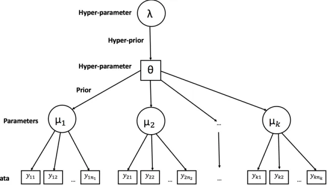
We give an example of hierarchical model using grouped data. Suppose, there are k
groups with possibly different number of observations. Let yij be the jth observation in
group i forj = 1,2, . . . , ni and i= 1,2, . . . , k. We model yij ∼f(µi), where f is a
probability distribution with parameter µi. Then,µ1, µ2, . . . , µk are the parameters and we
assigned each of them a prior distribution g such that µi ∼g(θ) whereθ is an
hyper-parameter. We could also assign a hyper-prior toθ with a parameterλ whose value
is fixed. In Fig. 1.1, we present the hierarchical structure for this model. This example was motivated by a similar setting in Fig.1 of Al-Amin et al. (2014).
Fig. 1.1: An exmaple of hierarchical model for grouped data
1.1.1 Prior, Likelihood and Posterior Distributions
There are three important parts in Bayesian inference: prior, likelihood, and posterior. A brief explanation of each part is provided in the following.
First of all, the prior distribution for any parameter θ, denoted by π(θ), is one’s initial beliefs about a probability distribution before information has been examined. For
example, our interest is in the probability distribution of voters in favor of a specific party in an upcoming election. There are several ways to get a prior distribution. For example, using information from past elections can help us to determine an appropriate prior distribution for the proportion of voters willing to support the party. We can also use the supposition of an expert, which will help us to select the prior distribution for the required model. Moreover, an uninformative prior, one which lacks available information, could be determined by equally weighing all possibilities. There are some priors that can be selected by certain qualities such as, the Jeffrey or Bernardo’s reference prior (Banerjee et al., 2014).
The likelihood function, the second factor in the Bayesian inference, describes the possibility of different values of a parameter solely from observed data.
The last factor of the Bayesian inference is the posterior distribution, which is denoted byπ(θ|D), where D is the data. We can think about the posterior distribution as a
modification of the prior distribution after the data are observed using the likelihood as a function of parameters. The posterior distribution is how we make inferences about unknown parameters.
When π(θ) is the prior distribution, and we have independent observations
x1, x2, . . . , xn, then f(D|θ) = n Q i=1
(f(xi|θ)) is the likelihood function, and π(θ|D) is the
posterior distribution. This formula was derived from the classic Bayes Theorem which is
π(θ|D, α) = R f(D|θ)h(θ|α)
f(D|u)h(u|α)du (1.1)
In summary, the prior distribution is the best way to guess the parameters before observing the data, and the posterior distribution is the one to use after observing the
data. This relationship can be written as follows:
P osterior ∝ Likelihood×P rior π(θ|D) ∝
n Y
i=1
(f(xi|θ))×π(θ)
Bayes theorem, or Bayes’s rule, is one of the most famous theorems in statistics. It is used to define the probability of an event by using the information about the prior distribution that may be related to the event. In this subsection, we will consider the following example to better understand the Bayesian Hierarchal model by using the Bayes theorem. If we want to determine the background for students in a math class, we need to get information about the student’s high school grades, then combine them with their current grade point average (GPA). This will give us an estimate for how well they did in the math class.
However, in many situations, the posterior π(θ|D) may not be a standard distribution. In those cases, it may become difficult to solve the problem analytically or numerically. Therefore, there is a special technique called the Monte Carlo Method which is used to
learn the properties of θ by drawing samples from π(θ|D) and then performing empirical
computation.
1.2 Monte Carlo Method for Bayesian
If we are uncertain about the inputs in any experiment, then we can simulate the posterior by using the Monte Carlo (MC) method (Gilks et al., 1995). The main objective of the MC method is to compute results based on repeated random sampling and statistical analysis. Monte Carlo Methods are used in high dimensional problems, and can often be used with other methods to complete analyses (Geman and Geman, 1984). The results of the many experiments that use the MC method simulation are not well documented. However, there are many applications that are difficult to integrate because they have complex hierarchical
structures. We will show two examples for posterior distributions; one for a binomial distribution and the other for a Poisson distribution.
1.2.1 Binomial Distribution Example
Let us considern independent binomial experiments with a different number of trials but
the same probability of success. Assume y1 was the number of success in the first
experiment out ofn1 trials, y2 the number of success in the second experiment out of n2
trials and so on. For simplicity we can write it as
yi ∼Bin(ni, p), where 0< p <1, and ni is known. We want to determine the posterior
distribution of p. The likelihood functionL(y) can be found by multiplying the n binomial
functions, so we can define it as follows:
L(y) = n Y i=1 f(yi) = n Y i=1 ni yi pyi(1−p)ni−yi (1.2)
We can choose beta to be the prior distribution. So, the prior distribution is
p∼Beta(a0, b0)
π(p)∝pa0−1(1−p)b0−1
We can get the posterior binomial distribution by multiplying the likelihood function and posterior distribution as follows:
π(p|y) ∝ L(y)π(p) ∝ n Y i=1 ni yi pyi(1−p)ni−yipa0−1(1−p)b0−1 ∝ pPni=1yi(1−p)Pni=1(ni−yi)pa0−1(1−p)b0−1 ∝ pPni=1yi+a0−1(1−p)Pni=1(ni−yi)+b0−1
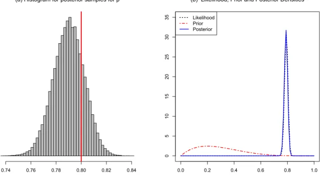
=Pn i=1yi+a0 and rate = Pn i=1(ni−yi) +b0. p|D∼Beta n X i=1 yi+a0, n X i=1 (ni−yi) +b0 (1.3) We applied the posterior distribution that we got in Eq. 1.3 for a dataset with 100
observations. The dataset was generated by a binomial distribution with p= 0.8. We used
the posterior to simulate samples of p, and we plotted the histogram in Fig.1.2-a. The
posterior samples mean of p is equal to 0.7899, and it lies inside the 95% credible intervals, which is (0.7654,0.8134). The red line marks the true value for p= 0.8. In Fig.1.2-b, we plotted the likelihood function and the prior distribution with rate = 2 and shape = 5 which were represented by the long red dashed line. It is clear that it was far from the data. We plotted the posterior density also, which was represented by the solid blue line, and it is very close to the likelihood function.
(a) Histogram for posterior samples for p
0.74 0.76 0.78 0.80 0.82 0.84 0.0 0.2 0.4 0.6 0.8 1.0 0 5 10 15 20 25 30 35
(b) Likelihood, Prior and Posterior Densities Likelihood
Prior Posterior
Fig. 1.2: Densities and Histogram for Binomial Distribution Example: red line denotes the true value from the simulation
1.2.2 Poisson Distribution Example
In a second illustration of Monte Carlo methods, we discussed the posterior inference for a Poisson model. Lets say yi ∼P oi(λ), wherei= 1,2, . . . , n. The likelihood function of y is
defined as follows: L(y|λ) = n Y i=1 f(yi|λ) = n Y i=1 exp(−λ)λ yi yi! = exp(−nλ)λ y1λy2. . . λyn y1!y2!. . . yn! = exp(−nλ) λ Pn i=1yi y1!y2!. . . yn!
Now let us consider that λ follows the gamma prior distribution such as λ∼Γ(a0, b0), with
density function f(λ) = b a0 0
Γ(a0)λ
(a0−1)exp(−b
0λ). As we can see, the prior distribution of λ is
expressed as π(λ)∝exp(−b0λ)λa0−1. Notice that the prior distribution of λ , π(λ), must
be a distribution that only allows positive values because λ can only be present with
positive real numbers.
After finding the likelihood function and the prior distribution, now we are ready to
derive the posterior distribution for λ|D by multiplying both of them as we can see below:
π(λ|y) ∝ L(y|λ)×π(y) = exp(−nλ) λ Pn iyi y1!y2!. . . yn! exp(−b0λ)λa0−1 = exp(−nλ)λPniyiexp(−b 0λ)λa0−1 = exp(−(n+b0)λ)λ Pn iyi+a0−1
distribution with shape = n P i yi+a0 and rate =n+b0. λ|D∼ Gam n X i yi+a0, n+b0 (1.4)
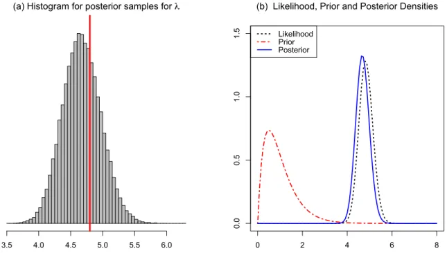
The simulation data that we applied in the above method has 50 observations. It was
generated by using a Poisson distribution with λ= 4.8. We used Eq. 1.4, to simulate
samples forλ, and we plotted the histogram for the posterior samples in Fig. 1.3-a. The
true value for λ= 4.8 was marked by the red line. The posterior sample mean, 4.6725, is
close to the true value and it lies in the 95% CI which is (4.1037,5.2729). In Fig. 1.3-b, we plotted the prior, likelihood and posterior distributions. The posterior distribution is very close to the likelihood function which indicates that the likelihood has much stronger influence on the final inference than the prior.
(a) Histogram for posterior samples for λ
3.5 4.0 4.5 5.0 5.5 6.0 0 2 4 6 8
0.0
0.5
1.0
1.5
(b) Likelihood, Prior and Posterior Densities Likelihood
Prior
Posterior
Fig. 1.3: Densities and Histogram for Poisson Distribution Example: red line denotes the true value from the simulation
it is not easy to sample from them directly. More commonly, a complex hierarchical model has many parameters. In that case, π(θ|D) is a high-dimensional posterior distribution. As described below, Markov Chain Monte Carlo is an efficient way to solve these types of problems.
1.3 Markov Chain Monte Carlo (MCMC)
The Markov Chain Monte Carlo (MCMC) method is useful when it is challenging to sample from the target posterior density. MCMC is one of the most important techniques in statistics, and it is used widely in many statistical applications. These kinds of methods are types of algorithms which work by sampling the probability distribution that is derived from a MC method (Gill et al., 2012). After several steps, the MCMC uses the chain as an approximate sample of desired distribution. The approximation improves after many steps are complete. In the remainder of this chapter, we will describe the three important
MCMC methods that we used in this thesis, which are Metropolis-Hastings, Gibbs sampling and slice sampling, with necessary theoretical justification.
1.3.1 Metropolis-Hastings (M-H)
One of the important types in MCMC algorithms is the Metropolis - Hastings (M-H)
algorithm. M-H works by drawing a sample from any proposal distribution q(θ|θold)
whereas the original target was to draw from another density p(θ). One of the most
important flexibilities which makes M-H more suitable is that it is adequate to knowp(θ)
up to a proportianality constant. That is useful because in some situations it is difficult to compute the necessary normalization factor. The process of the M-H algorithm works by creating samples one-by-one, moving from one sample to the next one. The algorithm uses a proposal distribution for the next sample that is dependent on the current sample value (Chib and Greenberg, 1995). This candidate will be either accepted or rejected based on
an acceptance probability. The probability of acceptance is determined by comparing the ratio of p(θ) at proposed and current values and the ratio of q(θ) at those values as well. Moreover, there is a special case of the M-H algorithm when the proposal function is symmetric which is called the Metropolis algorithm. We can summarize the M-H algorithm as follows. Algorithm 1 Metropolis-Hastings (M-H) INPUT: θ(i−1) = (θ(i−1) 1 , θ (i−1) 2 , . . . , θ (i−1) k ), q(x) OUTPUT: θ(i) = (θ(i) 1 , θ (i) 2 , . . . , θ (i) k ) θproposed ∼q(θproposed|θ)
R(θproposed, θ(i−1)) = min(1,p(θproposed)q(θ(−1)|θproposed)
p(θ(i−1))q(θproposed|θ(i−1)) ) u∼unif(0,1) if u≤R(θproposed, θ(i−1)),then θ(i) =θproposed else θ(i) =θ(i−1) end if 1.3.2 Gibbs Sampling
Gibbs sampling is a version of the MCMC method. The process is that if we are given a multivariate distribution, then we should divide the vector into several blocks and sample each block for its conditional distribution given other blocks. The idea in Gibbs sampling is to generate posterior samples by sweeping through each variable (or block of variables) (Carter and Kohn, 1994). Eventually, we reach a sample from its conditional distribution
with the remaining variables fixed to their current values. Suppose we have k parameters
θ1, θ2, . . . , θk, so Gibbs sampling can be found by first finding the joint posterior
Then, we update parameters one by one. For example, for θ1 and if we assume all other θ0s
are fixed at their current values, then we can find conditional posterior for θ1 which is
π(θ1|θ2, . . . , θk, D). We repeat this process for θ2 and then for θ3 until θk; so we havek
conditional posteriors. In the next step, we draw the rephrase symbol for each conditional distribution by using large numbers. That gives us posterior samples for each of
θ1, θ2, . . . , θk which we then analyze. In the following algorithm, we summarize the Gibbs
sampler steps.
Algorithm 2 Gibbs Sampler
INPUT: θ(i−1) = (θ(1i−1), θ2(i−1), . . . , θk(i−1)) OUTPUT: θ(i) = (θ1(i), θ(2i), . . . , θ(ki)) for i= 1,2, . . . , N do θ1(i) ∼p(θ1|θ (i−1) 2 , θ (i−1) 2 , . . . , θ (i−1) k ) θ2(i) ∼p(θ2|θ (i) 1 , θ (i−1) 3 , . . . , θ (i−1) k ) θ3(i) ∼p(θ3|θ(1i), θ (i) 2 , . . . , θ (i−1) k ) .. . θk(i) ∼p(θk|θ (i) 2 , θ (i) 2 , . . . , θ (i) k−1) end for
In the next section, we will show an example for Gibbs sampling with normal
distribution, where the two parameters µand σ have been estimated by the above steps.
1.3.3 Slice Sampling
Slice sampling is another method of the MCMC technique. It is a useful tool for drawing samples from a posterior distribution which is not easy to draw from (Neal, 2003). To understand slice sampling, let us consider the parameter θ with distributionf(θ). It is easy to use slice sampling if the following conditions are satisfied: f(θ) can be written as
we need to introduce a new random variable u.
f(u, θ) = π(u|θ)f(θ) =g(θ)h(θ) 1
h(θ)1(u < h(θ)) =g(θ)1(u < h(θ))
We can summarize the slice sampler steps by the following algorithm.
Algorithm 3 Slice Sampler
INPUT: θ(i−1) = (θ(i−1) 1 , θ (i−1) 2 , . . . , θ (i−1) k ) OUTPUT: θ(i) = (θ(i) 1 , θ (i) 2 , . . . , θ (i) k ) f(θ) =g(θ)h(θ) whereh(θ)>0 for i= 1,2, . . . , N do u∼unif(0, h(θ)) π(u|θ) = h(1θ)1(u < h(θ)) f(θ|u) = g(θ)1(θ ∈H(u)) where H(u) = h−1(θ) end for 1.4 Illustration Examples
We implement Gibbs sampling with a simulation from normal distribution. We summarize the result for posterior distributions by using diagrams.
1.4.1 Simulation Example from Normal Distribution Suppose, x1, . . . , xn ∼N(µ, σ2) where µ, σ2 unknown.
f(x) = √ 1 2πσ2 exp −1 2 (x−µ)2 σ2
In this example, we want to understand how Gibbs sampling works with a normal
function by multiplying the n densities functions. The likelihood function will be, f(x)∝ n Y i=1 1 √ 2πσ2 exp − 1 2 (xi−µ)2 σ2 (1.5)
Now, we assume appropriate priors for both unknown parameters. Let us assume that the prior for µis N(µ0, σ02). Inverse gamma is the conjugate prior distribution of variance of
the normal distribution. Because of this, we choose the prior distribution for σ2 to be
IG(a0, b0). µ ∼ N(µ0, σ02)∝exp 1 2 (µ−µ0)2 σ2 0 σ2 ∼ IG(a0, b0)∝ 1 (σ2)a0+1 exp −b0 σ2
We obtain the conditional posterior forµ, σ2 by multiplying the likelihood function by the
prior distributions of µ, σ2. Beginning with the conditional posterior for µ, the procedures
were derived by the posterior distribution for µshown below
π(µ|σ2, D) ∝ n Y i=1 exp− 1 2 (xi−µ)2 σ2 exp− 1 2 (µ−µ0)2 σ2 0 ∝ exp−1 2 Pn i=1(xi−µ) 2 σ2 exp1 2 (µ−µ0)2 σ2 0 ∝ exp−1 2 hPn i=1(x 2 i −2µµi+µ2) σ2 + µ2−2µµ0+µ20 σ2 0 i ∝ exp−1 2 hPn i=1(−2µxi+µ2) σ2 0 + µ 2−2µµ 0 σ2 0 i ∝ exp−1 2 h µ2(n σ2 + 1 σ2 0 )−2µ( Pn i=1xi σ2 + µ0 σ2 0 )i
For simplification, we will use, A= σn2 +
1 σ2 0 , and B = Pn i=1xi σ2 + µ0 σ2 0 , so the posterior
distribution for µwill be f(µ|σ2, D) ∝ exp−1 2 h Aµ2−2Bµi ∝ exp−1 2 h Aµ2−2B AAµ i ∝ exp−A 2 h µ2 −2B Aµ i ∝ exp−A 2 h µ2 −2B Aµ+ ( B A) 2i ∝ exp−A 2 µ−(B A) 2 ∝ exp−1 2 µ−(BA)2 1 A
From the above computation, the conditional posterior distribution for µgiven σ2 and the
data is also a normal distribution with mean equal to BA and variance equal to A1,
µ|σ2, D ∼N(B
A,
1
A) (1.6)
Second, we will find the posterior distribution for σ2 by fixing µ and the data by
following the same process as above.
π(σ2|µ, D) = 1 (σ2)12 exp−1 2 (xi−µ)2 σ2 × 1 (σ2)a0+1exp −b0 σ2 = 1 (σ2)n2 exp−1 2 Pn i=1(xi−µ) 2 σ2 × 1 (σ2)a0+1 exp −b0 σ2 = 1 (σ2)n2+a0+1 exp− 1 σ2 hPn i=1(xi−µ) 2 2 +b0 i
Apparent from this computation, the conditional posterior distribution for σ2 is an
inverse gamma with shape = n2 +a0, and scale =
Pn
i=1(xi−µ)2
posterior distribution for σ2 given µand the data (D) is σ2|µ, D ∼IG(n 2 +a0, Pn i=1(xi−µ)2 2 +b0) (1.7)
In this case, σ12 will follow the Gamma distribution with the same shape and rate. In other
words, sinceσ2 is an inverse gamma distribution, it follows that 1
σ2 is a gamma distribution. 1 σ2 ∼Γ( n 2 +a0, Pn i=1(xi−µ)2 2 +b0) (1.8)
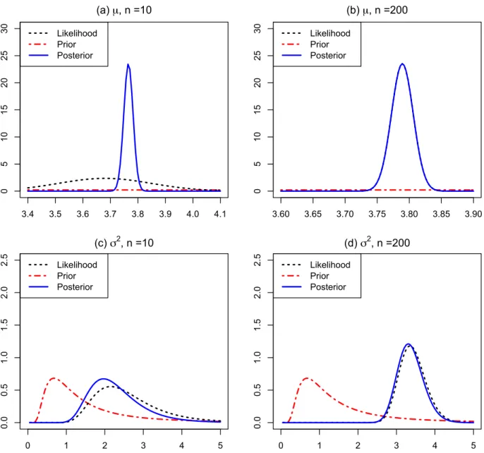
We can fit the Bayesian model based on the posterior distribution for µand posterior
distribution for σ2 that we derived above. We generated a simulation dataset with 200
observations by using the normal distribution with µ= 3.8 and σ2 = 4. In Fig. 1.4, we
plotted the likelihood function, prior distribution and the posterior distribution from a normal distribution with small and large datasets. We chose the initial parameters for
normal prior distribution to beµ=−10 andσ2 = 10, and for the inverse gamma
3.4 3.5 3.6 3.7 3.8 3.9 4.0 4.1 0 5 10 15 20 25 30 (a) µ, n =10 Likelihood Prior Posterior 3.60 3.65 3.70 3.75 3.80 3.85 3.90 0 5 10 15 20 25 30 (b) µ, n =200 Likelihood Prior Posterior 0 1 2 3 4 5 0.0 0.5 1.0 1.5 2.0 2.5 (c) σ2, n =10 Likelihood Prior Posterior 0 1 2 3 4 5 0.0 0.5 1.0 1.5 2.0 2.5 (d) σ2, n =200 Likelihood Prior Posterior
Fig. 1.4: Posterior samples distribution plots for µand σ2 with small and large sample size
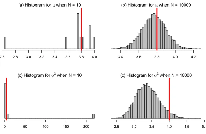
We used Eq.1.6 and Eq. 1.8 to simulate samples for µand σ2, respectively. The
resulting histogram shown in Fig.1.5 displays the fundamental difference for bothµ and σ2
when we chose a different number of iterations. When we had a small number of iterations,
the distributions of bothµand σ2 are unorganized (skewed), and it looks like a multi-model
as we can see in Fig. 1.5-(a,c). However, when we had a large number of iterations, we actually approached a normal distribution as we see in Fig. 1.5-(b,d). It is clear that they
are approximately symmetric. It is obvious that we need a large number of iterations in Gibbs sampling since our choices for the prior initial values were far away from the true values. In Fig. 1.5-(a-d), the true values for µ and σ2 are delineated by the red line.
(a) Histogram for µ when N = 10
2.6 2.8 3.0 3.2 3.4 3.6 3.8 4.0
(b) Histogram for µ when N = 10000
3.4 3.6 3.8 4.0 4.2
(c) Histogram for σ2 when N = 10
0 50 100 150 200
(c) Histogram for σ2 when N = 10000
2.5 3.0 3.5 4.0 4.5 5.0
Fig. 1.5: Histograms for posterior samples for µ and σ2 when N = 100 and N = 10000: red line denotes the true value from the simulation
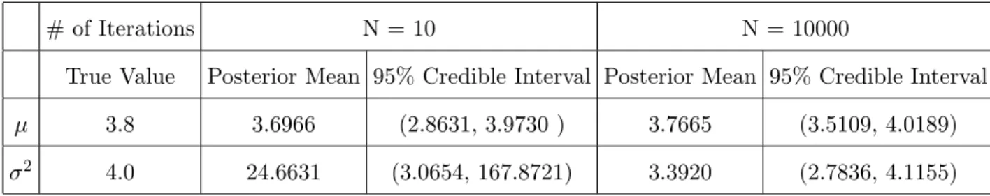
In Table 1.1, we included the true value, posterior mean and 95% credible intervals for
bothµ and σ2. The credible interval whenN = 10 is wider than the credible intervals
when N = 10000. This indicates that for a large number of iterations our posterior mean
Table 1.1: Comparison among true values, posterior means and 95% credible intervals when
N = 10 iterations vs. N = 10000 iterations
# of Iterations N = 10 N = 10000
True Value Posterior Mean 95% Credible Interval Posterior Mean 95% Credible Interval
µ 3.8 3.6966 (2.8631, 3.9730 ) 3.7665 (3.5109, 4.0189)
Chapter 2
Bayesian Inference in Regression
2.1 Introduction
Regression analysis is a statistical procedure to estimate the relationships between variables and how to use that relationship for predictive purposes. In general, regression analysis focuses on the relationship between a dependent variable and one or more independent variables, which are also known as the predictors. Regression analysis is important because it can help us understand the changes of a specific value of the dependent variable when an independent variable is altered, while the other independent variables remain constant (Vaughn, 2008). In this case, to model linear regression, we can use an advertising
expenditures example - advertising expense is the independent variable and the dependent variable is sales. This model can be useful for businesses making advertising decisions.
Depending on how many independent variables we are using, we refer to it as simple and multiple regression. Simple regression is used when we have only one independent variable while multiple regression is used when more than one independent variable is present. Moreover, the relationships among variables can be of different kinds - if the relationship is assumed to be in the form of a straight line then it can be defined by a linear regression model, while the nonlinear regression model can be defined by general curves between the variables (Vaughn, 2008). There are many different ways to approach a regression model. Some are simple, while others are quite complex, but all have the power to explain the response in different levels.
In this chapter, we will discuss MCMC algorithms for multiple linear regression which we are going to use as a starting point for developing outlier detection methods in Chapter
3.
2.2 Bayesian Inference of a Multivariate Linear Regression
In this section, we are going to focus on construction of a Gibbs sampler for multiple linear regression. The linear regression equation is
yi =β0+β1xi1 +· · ·+βpxip+i, wherei ∼N(0, σ2)
Forn observations, the multiple linear regression in matrix notations is, given by y, where
Y =Xβ+, where∼M V Nn(0n, σ2In)
such that Y is a n×1 vector, β is an (p+ 1)×1 vector, X is n×(p+ 1) matrix, 0n is zero
vector of length n, σ2 is a scalar value, and I
n isn×n identical matrix.
From above, we conclude that y∼M V Nn(Xβ, σ2In), so the likelihood function is
defined as follows: L(y) = n Y i=1 f(yi) = 1 (σ2)n2 exp−1 2(y−Xβ) T(σ2I n)−1(y−Xβ) = 1 (σ2)n2 exp −1 2(y−Xβ) TIn σ2(y−Xβ) = 1 (σ2)n2 exp−1 2 (y−Xβ)T(y−Xβ) σ2
We chose the prior for β as β ∼M V N(0, c0Ip+1), where c0 was chosen to be a large
conditional posterior distribution for β can be defined as follows: π(β|σ2, D) ∝ L(y)×Π(σ2|β, D) ∝ exp−1 2 h(y−Xβ)T(y−Xβ) σ2 + βTβ c0 i ∝ exp−1 2 hyTy−yTXβ−βTXTy+βTXTXβ σ2 + βTβ c0 i ∝ exp−1 2 h−yTXβ−βTXy+βTXTXβ σ2 + βTβ c0 i ∝ exp−1 2 h−2βTXTy+βTXTXβ σ2 + βTβ c0 i ∝ exp−1 2 h −2βTX Ty σ2 +β T(XTX σ2 )β+β T(I c0 )βi ∝ exp−1 2 h −2βTX Ty σ2 +β Ti ∝ exp−1 2 h −2βTX Ty σ2 +β T[XTX σ2 + I c0 ]βi By considering b = XσT2y and A= XTX σ2 + I
c0, we can rewrite the posterior distribution forβ as follows: π(β|σ2, D) ∝ f(y)×Π(σ2) ∝ exp(−1 2 h βTAβ−2βTbi) ∝ exp−1 2(β−p) Tφ(β−p) ∝ exp−1 2(β−A −1b)TA(β−A−1b)
The above equation matches the multivariate normal density with µ=A−1b and Σ =A−1.
Therefore, the full conditional posterior for β is
β ∼M V N(A−1b, A−1) where A= X TX σ2 + I c0 and b= X Ty σ2 (2.1)
G1 = (y−Xβ)T(y−Xβ), hence π(σ2|β, D) ∝ (σ2)−n2 exp − 1 2 G1 σ2 (σ2)−(a0+1)exp − b0 σ2 ∝ (σ2)−n2−(a0+1)exp − 1 σ2( G1 2 +b0) ∝ (σ2)−(n2+a0+1)exp − 1 σ2( G1 2 +b0)
The above formula is similar to the inverse gamma distribution with shape equal to n2 +a0
and rate equal to G1
2 +b0. So, the posterior distribution forσ 2 is σ2 ∼IG(n 2 +a0, G1 2 +b0) (2.2) 2.3 Illustrative Examples
We applied the Gibbs sampler that was developed above to two regression examples - one with a simulated dataset and another with a real dataset.
2.3.1 Example 1: Simulation Example with Three Covariates
In this example, we used the posterior distributions forµ andσ2 (Eq. 2.1 and Eq. 2.2). We
generated 250 observations by first simulatingx-variables uniformly with (0,1), and then
we used β = (2.5,−1.2,4.8,0.07) andσ2 = 0.16. Running the Gibbs sampler for 100000
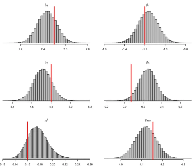
iterations, we acquired the posterior sample mean for all the parameters, which are
β0, β1, β2, β3 and σ2. We plotted the histograms for posterior samples of these parameters
in Fig. 2.1, and we marked the true values for these parameters by a red line. All the parameters in the posterior sample histograms were approximately normal, and the true values for the parameters were close to the samples mean. Moreover, we used the model to predict the response for selected x values of (1.23,0.12,0.37,0.32). The responses were plotted as histograms for the all the samples for the prediction, and we marked the true
value with the red line. β0 2.2 2.4 2.6 2.8 β1 -1.6 -1.4 -1.2 -1.0 -0.8 β2 4.4 4.6 4.8 5.0 5.2 β3 -0.2 0.0 0.2 0.4 0.6 σ2 0.12 0.14 0.16 0.18 0.20 0.22 0.24 0.26 ynew 4.0 4.1 4.2 4.3
Fig. 2.1: Posterior Histograms forβ0, β1, β2, β3, σ2 and ynew: red line denotes the true value from the simulation
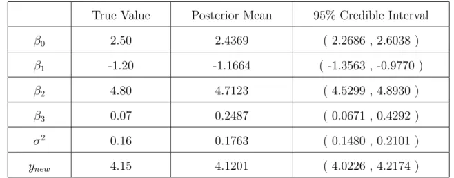
In Table 2.1, we compared the true values for our parameters with the posterior sample
means, and we created 95% CI for all the parameters and the prediction of ynew. All of the
Table 2.1: True Values, Predicted Values & 95% Credible Interval
True Value Posterior Mean 95% Credible Interval
β0 2.50 2.4369 ( 2.2686 , 2.6038 ) β1 -1.20 -1.1664 ( -1.3563 , -0.9770 ) β2 4.80 4.7123 ( 4.5299 , 4.8930 ) β3 0.07 0.2487 ( 0.0671 , 0.4292 ) σ2 0.16 0.1763 ( 0.1480 , 0.2101 ) ynew 4.15 4.1201 ( 4.0226 , 4.2174 )
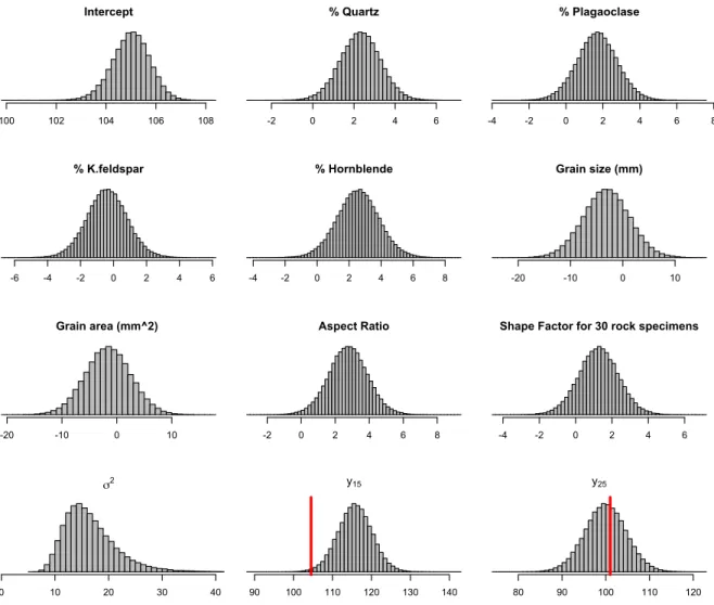
2.3.2 Example 2: Analysis of Rock Strength Dataset
We used the Gibbs sampler to analyze the Rock Strength Dataset (RSD). The RSD (Ali et al., 2014) contains information about the relationship between Uniaxial Compressive Strength (UCS) and 8 predictors, which are %Quartz, %Plagaoclase, %K.feldspar,
%Hornblende, Grain size (mm), Grain area (mm2), Aspect Ratio and Shape Factor for 30
rock specimens. First, we normalized the data, and then we ran the Gibbs sampler for 10000 iterations to create posterior samples for our parameters, which are
Intercept 100 102 104 106 108 % Quartz -2 0 2 4 6 % Plagaoclase -4 -2 0 2 4 6 8 % K.feldspar -6 -4 -2 0 2 4 6 % Hornblende -4 -2 0 2 4 6 8 Grain size (mm) -20 -10 0 10 Grain area (mm^2) -20 -10 0 10 Aspect Ratio -2 0 2 4 6 8
Shape Factor for 30 rock specimens
-4 -2 0 2 4 6 σ2 0 10 20 30 40 y15 90 100 110 120 130 140 y25 80 90 100 110 120
Fig. 2.2: Posterior Histograms for RSD: red line denotes the true UCS for test observations
In Fig. 2.2, we plotted the histograms for posterior samples for all the parameters in our model. It is clear that they are approximately symmetric with a large number of iterations. We checked our prediction by using leave-one-out-cross validation (LOOCV) by leaving out one of the observations and estimating the model with the rest of the
observations. In our example, we have 30 observations, which means we repeated the procedure 30 times. We found that 93% of the prediction of our samples lie inside the 95% credible intervals, which means that 28 of 30 prediction values lie inside the 95% CI. We
plotted the histogram for two posterior samples, y15 and y25, one lying inside the 95% CI
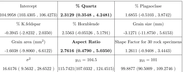
In Table 2.2, we show all the posterior means for all the parameters and the two prediction values. The most significant variables were % Quartz and Aspect Ratio.
Table 2.2: Predicted Values & 95% Credible Interval
Intercept % Quartz % Plagaoclase
104.9958 (103.4305 , 106.4273) 2.3129 (0.3548 , 4.2481) 1.6855 (-0.5103 , 3.8742)
% K.feldspar % Hornblende Grain size (mm)
-0.3945 (-2.8232 , 2.0350) 2.5563 (-0.05526 , 5.1791) -3.1271 (-11.8750 , 5.6153) Grain area (mm2) Aspect Ratio Shape Factor for 30 rock specimens
-1.6038 (-9.8060 , 6.6122) 2.7616 (0.4790 , 5.0350) 1.2611 (-0.9408 , 3.4443)
σ2 y15= 104.5 y25= 101
Chapter 3
Bayesian Model for Outliers in Regression
3.1 Introduction
In this chapter, we are focusing on detecting outliers from a large dataset using regression. Longitudinal studies are one of the common studies in many different types of research. A longitudinal study is useful to understand the changes of development over long periods of time such as days, weeks, months, or even years. The longitudinal studies are very useful for many health and medical issues. Obesity is a growing concern, and it is best measured with longitudinal studies. According to past research, approximately one in three children in the United States over two years of age are either overweight or obese (Ogden et al.,
2012). Arkansas has an even greater problem with childhood obesity, with 38.8% either
overweight or obese in the 2013-2014 school years. Moreover, there is a correlation between childhood obesity and adult obesity. Since this kind of study tracks people over long
periods of time, the longitudinal studies are very useful for studying obesity. But these kinds of studies are very sensitive because the data of these studies is changing over time. There are many elements that are affected by change over periods of time which will affect the results of the study. However, the biggest challenge in these kinds of studies is the occurrence of outlying observations. In fact, there are two different types of outliers in longitudinal studies, which are cross-sectional and longitudinal cross-sectional outliers. We can define the outliers as those observations that are different from the rest of the
observations of the same individual. There are several things that cause outliers, such as incorrect data entry, inappropriate measurements, and biased observations recorded on different individuals. These kinds of outliers can affect the results of an experiment. In this
chapter, we built models to be applied to datasets on height, weight, and BMI, gathered on public school children in the state of Arkansas to detect and eliminate cross-sectional and longitudinal outliers before the outliers can be used for analysis. We expect the models to be more sensitive to detect the outliers among heights as compared to weights. Because children of school age may have many elements that will affect their growth, children of the same age and in the same grade will not have the same measurments for height due to several factors, such as lifestyle, weight and genetics. Those factors can be added as covariates in regression. In this chapter, we will work with three different methods to detect outliers in heights and weights, and then suggest the best one for detecting outliers.
In regression, we can not consider an observation to be an outlier just because it has a very high/low value. Rather, an observation should be an outlier if compared to the rest of the data, it could not be explained by the covariates. Things would become more
challenging if the ability of the model to explain a response value depends on the covariates of the observation (systematic heteroscedasticity). We shall start with simpler hierarchical models without taking into account this type of behavior and then improve our model to address this.
3.2 Hierarchical Model for Outlier detection
We defined our multiple regression model as follows:
Y =Xβ+, where ∼M V Nn(0n,Σ)
where Σ is a diagonal matrix of σ2
i , i= 1, . . . , n. We allow every observation to vary
around the regression line. Because we tried to detect the outliers, we had a separate σ2
i for
every observation instead of having only oneσ2 for data entered. An outlier will be
corresponding σ2
i must be a large positive (because the mean for is zero which means σ2i
needs to be large to allow large positive or negative values of i.). Using a common σ2
would not achieve this constraint. In this case, our full posterior distribution will be as follows:
π(σ21, . . . , σ2n|D, β)∝L(D|β, σ12, . . . , σn2)π(σ12). . . π(σ2n) (3.1) To detect the outliers, we need to identify any positioni with large σ2
i.
There are many ways to solve this problem, but first we need to put a prior on eachσi2. There are two options for choosing appropriate prior distributions for each σi2. We will apply both options and refer to them as Method I and Method II.
For Method I, suppose that σ2
i follows an inverse gamma prior distribution with a
shape equal to a0 and rate equal to b0 ( i.e., σ2i ∼IG(a0, b0),i= 1, . . . n). So,
π(σi2) = (σi2)−a0−1×exp(−b0
σ2
i
) (3.2)
The likelihood function in this case can be written as:
L(y) ∝ |Σ|−12 exp −1 2(y−Xβ) TΣ−1(y−Xβ) ∝ (σ21. . . σn2)−12 exp −1 2(y−Xβ) Tdiag( 1 σ2 i )(y−Xβ), i= 1, . . . , n. ∝ (σ21. . . σn2)−12 exp −1 2 h yi−xT1β, y2−xT2β, . . . , yn−xTnβ i × diag( 1 σ2 i ) y1 −xT1β y2 −xT2β .. . yn−xTnβ ∝ (σ21. . . σn2)−12 exp −1 2 h(y1 −xT 1β)2 σ2 1 +(y2−x T 2β)2 σ2 2 +· · ·+(yn−x T nβ)2 σ2 n i
Hence, L(y) = (σ12. . . σn2)−12 exp −1 2 n X i=1 (yi−xTi β) σ2 i (3.3)
The parameters for this method were β, σ12,σ22,. . . ,σn2. To develop a Gibbs sampler, we first simulated the posterior distribution for β given the data and all σ2i, i= 1, . . . , n. Then we simulated the posterior distribution for σ2
i givenβ and the data. As we showed in
Chapter 2, the posterior conditional distribution forβ given the data andσ2
1, . . . , σn2 follows
a multivariate normal distribution, with a mean of A−1b and variance of A−1, ( i.e.,
β|σ2 1, . . . , σn2 ∼M V N(A −1b, A−1)). So, π(β|σ12, . . . , σn2, D) ∝ exp −1 2(β−A −1 b)T(β−A−1b) (3.4) where A=XTΣ−1X+In c0 and b =X TΣ−1y.
The posterior conditional distribution forσ2
1, . . . , σn2 givenβ and Dis derived as follows:
π(σ12, . . . , σn2|β, D) ∝ L(y)π(σ12). . . π(σn2) (3.5)
Now, from Eqs. 3.2, 3.3 and 3.5, we can compute the posterior distribution for
π(σ2 1, . . . , σn2|β, D) as follows, π(σ12, . . . , σn2|β, D) ∝ (σ12. . . σn2)−12 exp −1 2 n X i=1 (yi−xTi β)2 σ2 i (σ12)−a0−1exp −b0 σ2 1 × (σ22)−a0−1exp − b0 σ2 2 . . .(σn2)−a0−1exp − b0 σ2 n
Suppose we are interested in the posterior of σ2
1. We consider the terms that involve
only σ2
1 and ignore the other terms, so
π(σ12|β, σ22, σ32, . . . , σn2, D) ∝ (σ12)−12 exp −1 2 (y1−xT1β)2 σ2 1 (σ12)−a0−1exp − b0 σ2 1
∝ (σ12)−12−a0−1exp − 1 σ2 1 h(y1−xT 1β)2 2 +b0 i ∝ (σ12)−(12+a0)−1exp − 1 σ2 1 h −(y1−x T 1β)2 2 +b0 i
From the above formula, it is clear that the posterior distribution for σ2
1 is an inverse
gamma with a shape equal to a0 +12 and rate equal to
(y1−xT1β)2 2 +b0, σ12 ∼IG(a0+ 1 2, (y1−xT1β)2 2 +b0)
In general, the posterior conditional distribution for σ2
i, i= 1, . . . , n is an inverse gamma, σi2 ∼IG(a0+ 1 2, (yi−xTi β)2 2 +b0) (3.6)
From the above discussion, we can use the full conditional distribution for β and σ2,
which are represented in Eq. 3.3 and Eq. 3.6, respectively. We can summarize Method I by the following algorithm:
Algorithm 4 Method I
INPUT: Prior parameters a0, b0, c0 and initial values β and σ2.
OUTPUT: β, σ21, . . . , σ2n for i= 1,2, . . . , N do Given σ2 1, . . . , σ22 drawβ ∼M V N(A −1b, A−1) Given β drawσ2 j ∼IG(a0+12, (yj−XTjβ)2 2 +b0) end for
Suppose our model is
As we know, in a usual regression model the mean for i is equal to 0 and the variance is
equal to σ2. Now let us find the mean and the variance for Method I. The expectation for
i is still zero and the variance is σ2i. As we assumed,σi2 is a random variable and its prior
distribution wasIG(a0, b0), so the mean and the variance for inverse gamma are a0b−01 and
b0
(a0−1)2(a0−2), respectively. Since the σ
2
i is not a constant, we need to use the two formulas
below to find the mean and the variance.
E(y) =E E(y|x)
(3.7)
V ar(y) =E V ar(y|x)+ V ar(E(y|x)) (3.8)
From Eq. 3.7 and 3.8, we can compute the mean and the variance for i by replacingy
with i and x with σi2:
E(i) = 0 V ar(i) = E V ar(i|σi2) +V ar E(i|σ2i) =E(σi2) +V ar(0) = b0 a0−1
Therefore, for the i-th observation under Method I, the expected value for i is equal to
0, and the marginal variance is equal to b0
a0−1 .
For the second method, we can solve the problem using log(σ2
i) instead of working with
just σ2
i. That means that the simulated value for β does not change. The only thing that
will change is σ2
i.
log(σi2)∼N(µ0, σ20) whereδi = logσi2, i.e., σ
2
i = exp(δi)
likelihood function. L(y1) = (σ12) −1 2 exp −1 2 (y1−xt1β)2 σ2 1 = exp(δ1) −12 exp −1 2 (y1−xT1β)2 eδ1 = exp− δ1 2 exp−1 2exp(−δ1)(y1−x T 1β) 2
Since, the prior distribution forδ1 is
π(δ1) ∝ exp −1 2 (δ1−µ0)2 σ2 0 ∝ exp−1 2 δ2 1 σ2 0
The posterior distribution forδ1 is,
π(δ1|D) ∝ exp −δ1 2 exp − 1 2exp(−δ1)(y1−x T 1β) 2 exp −1 2 δ2 1 σ2 0 ∝ exp −1 2[ δ2 1 σ2 0 +δ1] exp −c1 2 exp(−δ1) , wherec1 = (y1−xt1β) 2 ∝ exp− 1 2σ2 0 [δ12+ 2δ1σ02] exp− c1 2 exp(−δ1) ∝ exp− 1 2σ2 0 [δ12+ 2δ1σ02+ (σ 2 0) 2−(σ2 0) 2]exp−c1 2 exp(−δ1) ∝ exp − 1 2σ2 0 (δ1+σ02) 2 exp −c1 2 exp(−δ1)
From the above formula, the first part represents the normal distribution, so
δ1 ∼N(−σ20, σ 2 0)f(δ1), wheref(δ1) = exp −c1 2 exp(−δ1)
π(δ1)∝N(δ1| −σ20, σ02)f(δ1), let us introduce variable u1 such that u1 ∼unif(0, f(δ1)), f(u1) = 1 f(δ1)
1
0< u < f(δ1) (3.9)Hence the posterior distribution for δ1 is
π(δ1|β, D) ∝ π(δ1)f(u1)
∝ N(−σ02, σ02)
1
0< u1 < f(δ1)
Notice that given δ1, we can compute f(δ1). Therefore, we can sample from
u1 ∼unif(0, f(δ1)). Now, the density function forδ1 is given by
f(δ1) = exp −c1 2 exp(−δ1) > u1 exp −c1 2e −δ1 >logu1 exp −δ1 < −2 c1 logu1 −δ1 <log −2 c1 logu1 δ1 >−log −2 c1 logu1
In this case, given the value of u1, we know the value of −log
−2
c1 logu1
. In conclusion, we can say the posterior distribution will be,
π(δ1|u1)∝N δ1| −σ02, σ20
1
δ1 >−log(− −2 c1 ) logu1 (3.10)From the above discussion, we can use Eq. 3.3, 3.9 and 3.10 to summarize Method II using the following algorithm.
Algorithm 5 Method II
INPUT: Prior parameters a0, b0, c0 and initial values β and σ2.
OUTPUT: β, ui and δi
for i= 1,2, . . . , N do
Given σ12, . . . , σn2 draw β ∼M V N(A−1b, A−1) Given β drawuj ∼unif(0, f(δi))
Given u1, . . . , un, β draw δj ∼N( δj σ2 0 , σ2 0)
1
f(δj)> uj end forFor the i-th observation, under Method II, the prior distribution for σ2
i was a log
normal distribution with mean µ0 and varianceσ02,
σ2i ∼LN(µ0, σ20)
The mean for σ2 is expµ
0+
σ2 0
2
, and by applying the same formula above(Eq. 3.7 and 3.8), we get, E(i) = 0 V ar(i) = E(V ar(i|σ2i)) +V ar(E(i|σi2)) =E(σ 2 i) +V ar(0) = exp(µ0+ σ2 0 2 )
3.3 Model for Outliers in presence of Systematic Heteroscedasticity
In this section, we will address a different method to (Method III) detect the outliers.
Previously, we assumed that variance of the error, σ2
i, i= 1, . . . , n, had no dependence on
any covariate. In this method, we allow the variance to change based on covariate values for each observation. Hence, an observation may have a large error even if it is not an outlier. Conversely, a true outlier may not have the largest error.
We assume that the diagonal entries of Σ will depend on covariates in the form function f.
We define, X(2) =
f(X1), f(X2), . . . , f(Xp)
, and model Σ = Diag((σ2
ieX
(2)T i ν))n
i=1;
Different choices of f give us a different model. We explore two choices (a) f(x) = X2 and
(b) f(x) =|X|.
Our parameters in this method are β, σ2
1, . . . , σn2 and ν. We chose the prior distribution
as follows: β ∼M V Np(0, c0I), σi ∼IG(a0, b0), and ν ∼M V Np(0, d0I).
After following the same processes that we did in Chapter 2, the posterior conditional distribution for β given the data and σ12, . . . , σ2n follow a multivariate normal distribution with a mean of A−1b and variance ofA−1, where A=XTΣ−1X+In
c0 and b =X TΣ−1y. The posterior distributionπ(β|σ2 1) is given by π(β|σ12, . . . , σn2, D)∝exp−1 2(β−A −1b)TΣ−1(β−A−1b) (3.11)
Similarly, we showed the posterior conditional distribution for σ2
i given β, ν and Das follows: π(σi2|β, ν, D)∝IG(a0+ 1 2, (yi−XiTβ)2 2 exp(Xi(2)Tν) + I c0 ), i= 1, . . . , n. (3.12)
Next, we found the posterior distribution forν by multiplying the likelihood function with
the prior distribution for ν. Since yi ∼N(XiT, σi2exp(X
(2)T
i ν)), the likelihood function L
isgiven by L(y1, . . . , yn) = n Y i=1 π(yi) = n Y i=1 (σ2i exp(Xi(2)Tν))−12 exp(−1 2 (yi−XiTβ)2 σ2 i exp(X (2)T i ν) ) ∝ n Y i=1 exp(−1 2X (2)T i ν) exp(−hiexp(−X (2)T i ν)), where hi = (yi−XiTβ)2 2σ2 i
Therefore, the posterior function π(ν|−) is given by π(ν|−)∝exp(−1 2 n X i=1 Xi(2)Tν) exp(− n X i=1 hiexp(X (2)T i ν)) exp(− 1 2 νTν d0 )
The logarithm posterior log(π(ν|−)) is given by
log(π(ν|−)) = −1 2 n X i=1 Xi(2)Tν− n X i=1 hiexp(X (2)T i ν)− 1 2 νTν d0 +constant (3.13)
We generated the proposed value ofν as
νjproposed ∼N(νjold, σ2proposed)
where (in MH) we accept the νproposed values as a new sample if
u < π(ν
proposed|−)
π(νold|−) , where u∼unif(0,1)
We can rewrite the above condition as follows,
log(u)<log(π(νproposed|−))−log(π(νold|−))
In Method III, we used two different functions, square and absolute value of covariates, as Methods III(a) and III(b). In reality, we do not know the correct functional form for the systematic heteroscedasticity (i.e., we do not know whether σ2 depends on X2 or|X|), so
we should consider all the possible cases to show a comparison. Since we used different form functions, we define method III(a) to use X(2) =X2 and Method III(b) to useX(2) =|X|.
Algorithm 6 Method III
INPUT: Prior parameters a0, b0, c0, d0 and initial values β, ν0 and σ2.
OUTPUT: β, σ2
1, . . . , σ2n and ν
for i= 1,2, . . . , N do
Given σ12, . . . , σn2 and ν draw β∼M V N(A−1b, A−1)
Given β and ν drawσ2
j ∼IG(a0+12, (yj−Xj(2)Tβ)2 2exp(Xj(2)Tν) + I c0 + I d0) ui ∼unif(0,1)
if log(ui)<log(π(νproposed))−log(π(νold)) then
νnew =νproposed else νnew =νold end if end for 3.4 Data Analysis 3.4.1 Simulation of Outliers
We used two simulation models to generate covariates for two main datasets, each with 800 observations. First of all, we generated 800 observations from a uniform distribution
between 0 and 1. Then, in Simulation Model I, we used β =c(0.5,−0.3,0.7,1.9) and
σ2 = 0.25 (i.e., the variance does not change), and we defined the model y as
y=Xβ+, where ∼M V Nn(0n, σ2In)
In the Simulation Model II, we used the same values ofβ that we used in Simulation
the model y as y =Xβ+, where∼M V Nn(0n,Σ), Σ =Diag((eX 2 i T ν))n i=1
From each main dataset we created two additional datasets by adding some outliers. First,
we created 4 randomly chosen outliers in each main dataset by increasing the 180th
observation by 4 and the 481st observation by 2.5, and by decreasing the 33rd and 653rd
observations by 3 and 2.75, respectively. We call them Dataset 1 and Dataset 2. We
created another version with more outliers than previous datasets. We increased the
percentage of outliers from 0.5% to 1% by adding 4 randomly chosen outliers to our
previous datasets, Dataset 1 and 2, where we decreased the 53rd observation by 2 and the
495th observation by 2.94, and increased 700th, 780th by 2.5, 2.1, respectively.
Fig. 3.1 and 3.3 contains the plot ofy and the plot of y versesXi, i= 1,2,3. As we can
see, it is easy to identify the outliers just by looking at them visually. In Fig. 3.2 and 3.4, when we plotted Dataset 2 and 4, it was difficult to identify the outliers because in many cases the outliers lie in the same region of most of the data, and there are other points that are not outliers which look more extreme. So, we expect Dataset 2 and 4 will be more challenging to find the outliers compared with Dataset 1 and 3.
Fig. 3.1: Dataset 1: the actual outliers are marked as red triangles
Fig. 3.3: Dataset 3: the actual outliers are marked as red triangles
3.4.2 Application of Methods on Simulated Datasets
We ran all methods with same the prior parameters, initial values and number of
iterations. For the prior parameters, we chose a0 = 2.1, b0 = 3, c0 = 10000 and d0 = 10000.
The initial values for β and σ2 were chosen to be the least-squares estimator. In Method
III, we chose the initial value for ν =c(0,0,0), and the value of σ2propose equal to 0.15, so that the MH achieved acceptance range between (30 - 40)%. The MCMC techniques were run for 10000 iterations where first 10% was discarded and the rest was thinned by 3.
First, we applied Method I and II for both Datasets 1 and 2, and as we see in Fig.3.5, both methods worked well with Dataset 1 since they could detect the exact outliers easily.
But they did not perform well with Dataset 2 because both of them did not use X at all in
Fig. 3.5: Outlier detection using posterior sample mean for σ2 for Method I and II for two simulation datasets: the actual outliers are marked as red triangles
Next, we applied Method III (a) and (b) for both Datasets, 1 and 2. For Dataset 1, both methods worked very well. Also, Method III (a), worked well with Dataset 1 because
we assumed X in the variance and with correct function form which is f(X) =X2.
because even though we usedX in the variance, we used misspecified function form,
f(X) = |X|.
Fig. 3.6: Outlier detection using posterior sample mean forσ2 for Method III (a) and III (b) for two simulation datasets: the actual outliers are marked as red triangles.
We ran the models for Datasets 3 and 4. In Fig. 3.7. We plotted the output for detecting outliers in Method I and II. With Dataset 3 both methods worked well as
expected. However, with Dataset 4, we noticed that both methods did not perform well since many data points lay above the outliers.
Fig. 3.7: Outlier detection using posterior sample mean for σ2 for Method I and II for two simulation datasets: the actual outliers are marked as red triangles.
We ran Method III (a) and (b) for Datasets 3 and 4. In Fig. 3.8, we notice that both
were far from other values. But, in Dataset 4, Method III (a) could detect easily only 5 outliers, and Method III (b) could detect only 4 outliers, and it did not perform as well as Method III(a) due to misspecified function form.
Fig. 3.8: Outlier detection using posterior sample mean forσ2 for Method III (a) and III (b) for two simulation datasets: the actual outliers are marked as red triangles.
number of outliers were known to us. In our simulation, there were 4 and 8 outliers as we
explained in Sec. 3.4.1. The x-coordinate represents the number of outliers that can be
identified in the model, and the y-coordinate represents how many observations we should
consider in the model, so we could catch all the outliers. We observed that all methods worked well with Dataset 1. Also Method III (a) worked well with dataset two since
Dataset 2 depends on X. Method III (b) does not work well compared to Method III (a)
for dataset two, but it is still much better than Method I and II for all Datasets 2, and 4.
Table 3.1: Comparison of detecting outliers across different methods and different datasets
# Outliers Dataset Method I Method II Method III (a) Method III (b)
4 1 ( 4 , 4 ) ( 4 , 4 ) ( 4 , 4 ) ( 4 , 4 ) 2 ( 0 , 36 ) ( 0 , 40 ) ( 3 , 6 ) ( 2 , 13 ) 8 3 ( 8 , 8 ) ( 8 , 8) ( 8 , 8 ) (8 , 8 ) 4 ( 0 , 393 ) ( 1 , 401 ) ( 5 , 304 ) ( 4 , 316 )
3.5 Estimation of Regression Coefficients
We want to analize how presence of outliers influence the estimation of regression coefficients. We used the same two simulation models that we described in Sec.3.4 to generate covariates for four datasets. Each dataset had 3 covariates, and for each covariate, we generated 800 observations from uniform distribution between 0 and 1. Then in the simulation model I,
y =Xβ+, where∼M V Nn(0n, σ2I)
we used β =c(0.2,−0.8,5.7,0) andσ2 = 0.25 (i.e., the variance did not change for all the
observations). We added noise to some of the observations to create outliers. The dataset with 8 outliers was denoted as Dataset 5 and the dataset with 40 outliers was denoted as Dataset 6. After running Method I, II, III(a) and III(b), we compared the true parameters
used in the simulation with the posterior means and 95% CI that we got from MCMC. The results were presented in Table 3.2 below.
Table 3.2: Comparison of parameters estimation across different datasets and different methods
Parameters True values
Dataset 5
Method I Method II Method III(a) Method III(b)
β0 0.2 0.24(0.057,0.426) 0.248(0.049,0.453) 0.155(0.069,0.242) 0.174(0.097,0.253 )
β1 -0.8 -0.876(-1.062,-0.679) -0.886(-1.093-0.684) -0.815(-0.891,-0.738)-0.832(-0.904,-0.761)
β2 5.7 5.730(5.536,5.927) 5.719(5.518,5.922) 5.785(5.705 ,5.861)5.775(5.702,5.848)
β3 0 -0.045(-0.236,0.149) -0.043(-0.252,0.160) 0.001(-0.068,0.072) -0.005(-0.073,0.063)
Parameters True values
Dataset 6
Method I Method II Method III(a) Method III(b)
β0 0.2 0.226(0.039,0.418) 0.225(0.067,0.383) 0.162(0.061,0.264) 0.178(0.086,0.268)
β1 -0.8 -0.866(-1.059,-0.665)-0.865(-1.024,-0.696)-0.814(-0.898,-0.727)-0.832(-0.913,-0.748)
β2 5.7 5.735(5.539,5.938) 5.737(5.572,5.893) 5.776(5.685,5.864) 5.771(5.685,5.856)
β3 0 -0.0492(-0.239,0.151)-0.038(-0.203,0.121) -0.006(-0.088,0.074) -0.012(-0.091,0.065)
In Table 3.2, we found that there were more parameters outside the 95% credible interval when we increased the number of outliers from 8 to 40. Also, we saw that the 95% credible interval for all β1, β2 and β3 got wider in Method III(a) and III(b) when we
compared Dataset 5 with 6.
Similarly, we generated two datasets from simulation model II,
y=Xβ+, where ∼M V Nn(0n,Σ), Σ =Diag((eX (2) i T ν))n i=1
where we used the same value of β and we used ν =c(0.8,3.75,0). By adding 8 and 40 outliers to the dataset, we got two datasets, we denoted them as Dataset 7 and 8,
the true parameters used in the simulation with posterior means and their 95% credible interval that we got from MCMC. The results were reported in Table 3.3 below.
Table 3.3: Comparison of parameters estimation across different datasets and different methods
ParametersTrue values
Dataset 7
Method I Method II Method III(a) Method III(b)
β0 0.2 0.281(0.003,0.554) 0.606(0.460,0.777) 0.288(-0.0640,0.630) 0.290(-0.085,0.657) β1 -0.8 -1.236(-1.560,-0.911)-1.632(-1.804,-1.463)-1.183(-1.642,-0.725)-1.236(-1.714,-0.766) β2 5.7 6.47(6.106,6.828) 5.836(5.736,6.124) 6.096(5.542,6.622) 6.109(5.553,6.631) β3 0 -0.281(-0.600,0.032) -0.483(-0.727,-0.355) -0.13(-0.572,0.291) -0.097(-0.555,0.362) ν1 0.8 — — 1.011(0.698,1.337) 0.522(0.205,0.860) ν2 3.75 — — 3.534(3.205,3.838) 3.165(2.833,3.483) ν3 0 — — 0.265(-0.081,0.611) -0.266(-0.610,0.043) ParametersTrue values Dataset 8
Method I Method II Method III(a) Method III(b)
β0 0.2 0.204(-0.081,0.483) 0.425(0.327,0.555) 0.2144(-0.147,0.580)0.221(-0.173,0.612) β1 -0.8 -1.144(-1.480,-0.815)-1.473(-1.579,-1.322)-1.064(-1.559,-0.580)-1.146(-1.648,-0.634) β2 5.7 6.465(6.092,6.836) 6.283(6.083,6.454) 6.077(5.494,6.625) 6.101(5.510,6.659) β3 0 -0.176(-0.500,0.141) -0.247(-0.354,-0.097)-0.060(-0.531,0.387)-0.023(-0.519,0.460) ν1 0.8 — — 1.107(0.790,1.433) 0.591(0.278,0.926) ν2 3.75 — — 3.454(3.129,3.772) 3.055(2.728,3.387) ν3 0 — — 0.509(0.157,0.855)-0.014(-0.360,0.328)
In Table 3.3, we can see that anything not covered in Dataset 7 still was not covered in
Dataset 8, and one extra parameter ν3 was not covered in Dataset 8. Also, the credible
Chapter 4
Future work
4.1 Analysis of Longitudinal Data on Student Biometrics
As discussed in the beginning of Chapter 3, the eventual aim of developing these methods was to apply them on a large dataset related to school students in Arkansas that is yet to be made available to us. The dataset contains the height, weight and BMI measurements of school students across different counties. It is temporal as well, as the same student’s biometric information is measured at different grades of his/her school years are recorded. Our goal is to detect the outliers in this dataset by using previously developed techniques. In the following, we first describe the necessary transformation in the raw data before using it in the model. Then, we discussed some practical challenges that we have to address.
4.1.1 Formulation of the Problem
Direct use of raw biometric measurements such as height or weight can pose some
challenges. Lets consider height - denote by Hi(t) the height of student i at grade t. The
change between two time points is ∆it which will be defined as ∆it=Hi(t+ 1)−Hi(t).
Obviously any negative value of ∆ is an outlier. A small positive value is acceptable but a large positive value is an outlier. Hence, working with ∆ implies we cannot treat the positive and negative values in the same way, so using a symmetric distribution like a
Normal model will not be reasonable. To remove this problem, we decided to useZ-scores
of heights instead of actual heights. These Z-scores are computed based on the quantile of
a student’s height calculated using database of student biometric across the entire country.
height of a randomly selected student in that country-wise database. Now, let us define
Yi(t) = Zi(t+ 1)−Zi(t). Our goal is to see if Yi changes too much (large absolute value).
The advantage of working with Y compared to ∆ is that large positive and negative
changes inY are equally likely a priori to be an outlier, so we do not have an issue with
using error distribution which is symmetric around 0. The outlier-detection model will be as follows,
Yit =β0+β1Xit(1)+· · ·+βpXit(p)+it, where it ∼N(0, σit2),
where {Xit(1), ..., Xit(p)} can be covariates such as gender, race, diet, sports activity indicator, school zip code, etc. Some of them will change over time whereas the others will be same for a student irrespective of grades. The outlier can be specific to both subscripts t and i. It is possible that a student’s height information at one grade is an outlier, whereas in the rest of the grades it is in the normal range.
4.1.2 Further Discussion
We anticipate some challenges in our modeling effort. For example, height and weight are not expected to show similar variation across time. A student’s weight can increase or decrease significantly between two successive measurements due to events such as diet
change, disease or surgery. We can see large positive or negative values in Y for weight
that may not be outliers. Therefore, it will be relatively difficult to identify true outliers in weight data as opposed to the data for heights.
Finally, we plan to validate the model results for the real datasets. Unlike the simulation data, we have no knowledge of the true outliers or their numbers. Because of this we need to develop some validation strategy in this setting. One option could be to identify the top 1% of data points based on the largest values of E(σ2
i|Y) and obtain
external expert evaluation to see how many of them are actually outliers. Alternative validation procedures based on statistical techniques are also being explored.