https://doi.org/10.5194/os-15-1023-2019 © Author(s) 2019. This work is distributed under the Creative Commons Attribution 4.0 License.
Using canonical correlation analysis to produce dynamically based
and highly efficient statistical observation operators
Eric Jansen1, Sam Pimentel3, Wang-Hung Tse3, Dimitra Denaxa4, Gerasimos Korres4, Isabelle Mirouze2, and Andrea Storto2
1Ocean Predictions and Applications (OPA) division, Euro-Mediterranean Center on Climate Change (CMCC), Lecce, Italy 2Ocean Modelling and Data Assimilation (ODA) division, Euro-Mediterranean Center on Climate Change (CMCC),
Bologna, Italy
3Trinity Western University (TWU), Langley, BC, Canada 4Hellenic Centre for Marine Research (HCMR), Athens, Greece
Correspondence:Eric Jansen ([email protected])
Received: 31 December 2018 – Discussion started: 23 January 2019
Revised: 28 May 2019 – Accepted: 18 June 2019 – Published: 2 August 2019
Abstract.Observation operators (OOs) are a central compo-nent of any data assimilation system. As they project the state variables of a numerical model into the space of the observa-tions, they also provide an ideal opportunity to correct for effects that are not described or are insufficiently described by the model. In such cases a dynamical OO, an OO that interfaces to a secondary and more specialised model, often provides the best results. However, given the large number of observations to be assimilated in a typical atmospheric or oceanographic model, the computational resources needed for using a fully dynamical OO mean that this option is usu-ally not feasible. This paper presents a method, based on canonical correlation analysis (CCA), that can be used to generate highly efficient statistical OOs that are based on a dynamical model. These OOs can provide an approximation to the dynamical model at a fraction of the computational cost.
One possible application of such an OO is the modelling of the diurnal cycle of sea surface temperature (SST) in ocean general circulation models (OGCMs). Satellites that measure SST measure the temperature of the thin uppermost layer of the ocean. This layer is strongly affected by atmospheric conditions, and its temperature can differ significantly from the water below. This causes a discrepancy between the SST measurements and the upper layer of the OGCM, which typ-ically has a thickness of around 1 m. The CCA OO method is used to parameterise the diurnal cycle of SST. The CCA OO is based on an input dataset from the General Ocean
Turbu-lence Model (GOTM), a high-resolution water column model that has been specifically tuned for this purpose. The parame-terisations of the CCA OO are found to be in good agreement with the results from the GOTM and improve upon existing parameterisations, showing the potential of this method for use in data assimilation systems.
1 Introduction
Many different types of OO exist. In its simplest form, an OO could just select one of the state variables in a point near the observation or, perhaps, perform an interpolation. More complex OOs may include corrections for processes that in-fluence the observation but are not modelled or are insuffi-ciently modelled. Ultimately, one could even consider a dy-namical OO that wraps a second numerical model to locally refine the results of the parent model. The latter solution may very well provide the most accurate results, but the vast num-ber of observations that need to be assimilated in a typical at-mospheric or oceanographic model means that this approach would require a prohibitive amount of computing resources. This limits OOs in most practical applications to relatively simple parameterisations in terms of the model state vari-ables. Moreover, variational data assimilation requires ob-servation operators to be linearised around the background within the inner loops (tangent-linear approximation). This translates into a need to construct OOs that can be formally and practically differentiated.
This paper presents a method of parameterising the results of a specialised model in such a way that it can be efficiently used within an OO. The parameterisation is based on canoni-cal correlation analysis (CCA), a well-established mathemat-ical method for finding cross-correlations between datasets. A new pseudo-dynamical OO is generated using the canon-ical correlation between the inputs and outputs of the spe-cialised model on a large and representative dataset. Once this correlation has been calculated, the application of the pseudo-dynamical OO involves only a matrix multiplication that can be performed at a fraction of the computational cost of the dynamical OO. A similar method has been used previ-ously to build reduced-order OOs in atmospheric data assim-ilation (Haddad et al., 2015).
This work is part of the SOSSTA (Statistical-dynamical observation Operator for SST data Assimilation) project, funded by the EU Copernicus Marine Environment Monitor-ing Service (CMEMS) through the Service Evolution grants. The aim of SOSSTA is to formulate an efficient OO for sea surface temperature (SST) DA that accounts for the diurnal variability of the ocean skin temperature. The results of the project are presented in multiple publications. The modelling of the diurnal cycle of SST is described in Pimentel et al. (2019), while the current paper focuses on the method for constructing the OO. The project includes pilot studies in the Mediterranean Sea and the Aegean Sea that will be described in forthcoming publications.
The paper is organised as follows: Sect. 2 provides a quick review of CCA; Sect. 3 discusses how CCA can be used to construct the OO matrix; Sect. 4 applies the CCA OO to the modelling of satellite sea surface temperature (SST) mea-surements in oceanographic models; and Sect. 5 discusses the performance of the method and other possible applica-tions. Conclusions are presented in Sect. 6.
2 The CCA method
CCA (Hotelling, 1936) is a method to find cross-correlations between two datasetsXandY. The datasets are considered to be matrices structured such that the columns represent dif-ferent variables and the rows represent the measurements of these variables. CCA then aims to find transformation matri-cesAandBthat transform the anomaly of the variables ofX andY, denotedX0andY0, into the set of canonical variables FandG:
F=X0A G=Y0B. (1)
The structure ofFandGmatches that ofXandY. The canonical variables are constructed such that the variableFi
is maximally correlated with the variableGi. At the same
time, bothFi andGi are uncorrelated withFj andGj for i6=j; therefore, each additional canonical variable describes the maximal remaining correlation between the two datasets. The number of canonical variables that can be obtained with this procedure is limited to the smallest number of variables inXorY.
The calculation of the matrices A and B is relatively straightforward using the algorithm of Björck and Golub (1973). Writing the requirements outlined above in equation form yields
FTF=GTG=I, (2a)
FTG=D, (2b)
withIthe unit matrix andDa diagonal matrix. The algorithm uses a QR decomposition to decompose bothX0andY0into an orthogonal matrixQand an upper-triangular matrixR:
X0=QxRx Y0=QyRy. (3)
The algorithm proceeds by applying a singular value decom-position (SVD) on the productQTxQy:
QTxQy=USVT. (4)
By trying the ansatz,
A≡R−x1U B≡R−y1V, (5)
the orthonormality requirement of Eq. (2a) becomes FTF=ATX0TX0A
=
UTR−x1T
RTxQTx(QxRx)
R−x1U =I,
(6)
and an analogous result follows forGTG.
The orthogonality requirement of Eq. (2b) becomes D=FTG=ATX0TY0B
=
UTR−x1T
RTxQTx QyRy
R−y1V
=UTUSVTV=S.
Therefore, the ansatz of Eq. (5) is a valid solution for the ma-tricesAandB. Moreover, by counting the number of degrees of freedom in these matrices and the number of constraints provided by Eq. (1), it can be shown that all solutions are permutations of Eq. (5) (Press, 2011). The canonical basis is therefore uniquely defined. In the case thatXandYcontain different numbers of variablesNxandNy, the SVD of Eq. (4)
selects theN largest correlations, withN=min(Nx, Ny).
As QR decomposition and SVD are common matrix op-erations that are efficiently implemented in most numerical libraries, this algorithm is straightforward to implement in most programming languages.
3 Using CCA to construct an OO
The CCA method can be used to construct an OO. LetXbe a set of (possibly) relevant model state variables and Ythe corresponding observation values. HereYcould be obtained from a specialised model but also from a historical dataset of real observations. Applying the algorithm of Sect. 2 yields the matricesA,B, andD. The first two convert the mean sub-tracted model states X0 and observation valuesY0 into their canonical counterpartsFandG. The diagonal matrixDholds for each pair of canonical variablesithe best fit to the slope of the correlation:Dii=dGi/dFi.
Assuming thatNx≥Ny – i.e. the number of model state
variables is at least equal to the number of observed variables – it is possible to calculateY0 fromX0 by passing through canonical space and applying the fitted slopeD,
Y0=X0ADB−1≡X0M, (8)
defining the CCA OO matrix,
M≡ADB−1, (9)
of sizeNx×Ny. As the CCA considers only the anomaly ofX
andY, an additional offset term needs to be considered to ac-commodate the mean values ofXandYin the input dataset. However, the mean values ofXandYcan be combined by applying the matrixM:
Y−Y=
X−XM Y=XM+K,
(10)
with
K≡Y−XM, (11)
a combined offset vector of lengthNy.
During the training phase of the CCA OO, the datasets X andYare used to calculate the matrix Mand the offset K. Once computed, they can be used to form an observation operator H that transforms a statexas
H(x)=xM+K. (12)
Furthermore, the tangent-linear approximation used in varia-tional DA schemes requires that
H(x)∼H(xb)+H0dx, (13)
whereH0is the tangent-linear version of the OO,xbthe back-ground state, and dxthe deviation from the background. The CCA OO is straightforward to implement in this scheme, since forH0and its adjointH0T it follows that
H0=MT H0T =M. (14)
4 Use case: satellite SST
One possible application of the new CCA OO is the assimi-lation of SST in ocean general circuassimi-lation models (OGCMs). In recent years OGCMs have seen significant improvements in vertical resolution, particularly near the surface, where the first layer has been reduced to a thickness of the order of 1 m or less. At this resolution, the diurnal cycle of SST should be taken into account. Although diurnal variability is included to some extent (Marullo et al., 2014), the vertical resolution of OGCMs is still insufficient to fully resolve the variability of the skin and subskin ocean temperature.
This issue becomes particularly evident when assimilat-ing satellite SST observations. The different types of sen-sors used on satellites probe the ocean temperature at dif-ferent depths. Infrared (IR) sensors measure the tempera-ture at about 10 µm, a layer that is referred to as the ocean skin. Microwave (MW) sensors, on the other hand, measure the temperature of the layer below that, the subskin, with a depth of about 1 mm. This is much shallower than the ver-tical resolution of a typical OGCM, while these layers are strongly affected by the atmospheric conditions. The ocean skin cools due to thermodynamic processes at the air–sea in-terface, while the absorption of solar heat causes a warm-ing of the subskin. At the same time, wind can mix the skin and subskin with the water below, smoothing the tempera-ture variations. During days of low wind and/or high insola-tion condiinsola-tions the amplitude of the SST diurnal cycle can be larger than the combined accuracy of the model and ob-servations, causing a straightforward assimilation of SST to degrade the performance of the model (Marullo et al., 2016). Under favourable conditions this amplitude is typically of the order of a few degrees (see e.g. Flament et al., 1994), but values as high as 6◦C have been observed (Merchant et al., 2008).
An important source of SST observational data is the Spning Enhanced Visible and Infrared Imager (SEVIRI) in-strument onboard the Meteosat satellites of the second gen-eration. As these are geostationary satellites, SEVIRI can provide continuous measurements of the same area with a 15 min temporal resolution. Although the IR imager is sensi-tive to skin temperature, the calibration algorithm of SEVIRI corrects for the cool-skin bias, and the resulting SST products should be considered the subskin temperature (Saux Picart and Legendre, 2018). For wind speeds greater than 6 m s−1 the skin temperature may be calculated asTskin=Tsubskin−
0.17◦C (Donlon et al., 2002), but this is only an approxima-tion.
This section will discuss how to use the output of a water column model specifically tuned for modelling the diurnal cycle of SST together with the CCA OO to build an observa-tion operator for SST that accounts for the diurnal variability. 4.1 General Ocean Turbulence Model
The SST diurnal cycle is modelled using the General Ocean Turbulence Model (GOTM). The GOTM is a one-dimensional water column model that includes multiple tur-bulence closure schemes (Burchard et al., 1999; Umlauf et al., 2005). It has been successfully adapted to model the near-surface variability of ocean temperature, including both the diurnal cycle and the cool-skin effect (Pimentel et al., 2008a, b). Recently it has been used to systematically sim-ulate the atmospheric and oceanographic conditions in the Mediterranean Sea (Pimentel et al., 2019). The latter study has resulted in a multi-year dataset modelling the diurnal cy-cle in the Mediterranean Sea on a grid of 0.75◦×0.75◦ reso-lution with hourly time resoreso-lution. For this dataset the GOTM is configured with thek-εturbulent kinetic energy parameter-isation with internal waves. The top 75 m of the water column is resolved using 122 vertical layers with fine resolution near the surface and gradually becoming coarser with depth. The uppermost 1 m contains a total of 21 layers, with the highest level at 1.5 cm of depth. This dataset is used in the present paper to build the CCA OO for SST.
The subskin SST represents the temperature at the base of the conductive laminar sub-layer of the ocean surface; for practical purposes it is represented by the temperature of the top model layer of the GOTM (1.5 cm). The conductive sub-layer of the air–sea interface, associated with the cool-skin effect, is parameterised and dynamically computed within the GOTM to produce a modelled skin SST. Further details are provided in Pimentel et al. (2019).
4.2 Operator setup
The aim for the CCA OO is to parameterise the IR and MW satellite SST observations as a function of temperature in the water column below. While the dataset of Pimentel et al. (2019) uses a fine vertical resolution to calculate the SST
ob-servations, the CCA OO will consider only the levels of a typical OGCM. Within the SOSSTA project this OGCM is the CMEMS Mediterranean Forecasting System (MFS) (Si-moncelli et al., 2014), but the parameterisation can be per-formed for any vertical distribution of levels.
The magnitude of the diurnal signal depends strongly on the atmospheric conditions, most importantly the insolation and wind speed. Insolation causes the ocean skin to heat up during the course of the day, while wind mixes the upper lay-ers of the ocean, leading to the dissipation of the heat. Due to latent heat loss, the ocean skin may even cool down be-low the bulk temperature. To accommodate a non-linear de-pendence on the different insolation and wind scenarios in the CCA OO, the GOTM dataset is divided into 12 insola-tion and 8 wind categories. Insolainsola-tion and wind are defined in each location as the daily mean value in local mean time (LMT). The category boundaries were chosen to equally di-vide the dataset. The magnitude of the diurnal warming for the different categories is shown in Fig. 1.
The GOTM dataset has been compared to SEVIRI data at the skin level in Pimentel et al. (2019) and was found to be in good agreement over the whole period of 2013 and 2014. However, after dividing the dataset into atmospheric cate-gories, it is found that categories with high diurnal warming may have a warm bias of up to 0.5◦C and categories with low diurnal warming a cold bias of typically 0.1–0.2◦C. This category bias is corrected for by subtracting the mean differ-ence between SEVIRI and GOTM at subskin level for each category.
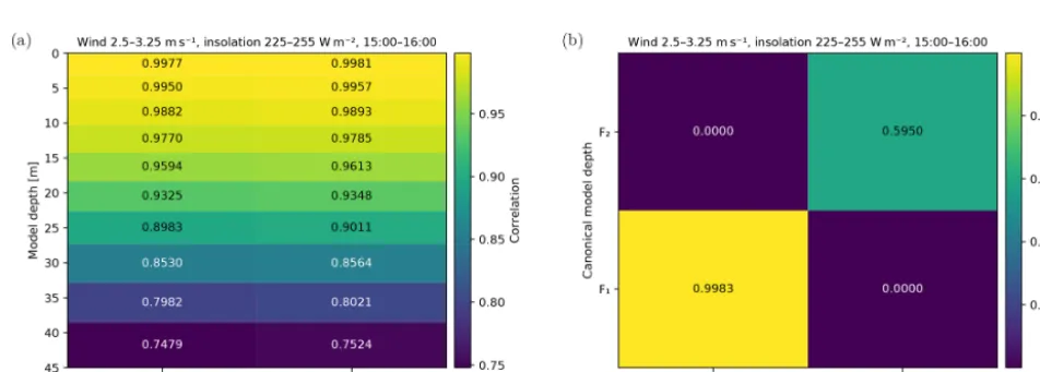
For each category of wind and insolation, and at hourly time resolution, the CCA OO is calculated to project the 10 uppermost levels of the MFS model onto the skin and sub-skin SST temperatures. The 10 levels extend down to a depth of approximately 40 m, which was chosen to be well below the depth influenced by the diurnal cycle of temperature. Fig-ure 2a shows the correlation between the model temperatFig-ure at various depths and the two SST observation types. As ex-pected, the SST is strongly correlated with the highest lev-els and the correlation decreases with depth. It is important to note that in this case the various levels are also strongly correlated with each other. Figure 2b shows the correlation after transforming to canonical coordinates. It can be seen that the strongest correlation has not significantly changed, as the first canonical variable is very similar to the highest model level. The second pair of canonical variables(F2,G2),
however, describes an additional correlation of around 60 % between model water temperature and SST.
4.3 Validation
Figure 1.The magnitude of the diurnal warming at the subskin level as a function of the time of the day for different wind and insolation categories. The diurnal warming is measured with respect to the SST at local sunrise. The wind categories are represented by the different panels, while the insolation categories are shown as different curves within each panel.
Figure 2.The correlation coefficients between the model variables and observations(a), with the canonical equivalent of these variables(b).
calculation. The GOTM dataset is split in two, withholding every other profile in the zonal direction from the calculation. The validation then uses the withheld profiles and extracts the depths corresponding to the MFS levels, mimicking the use of the operator inside a DA system. The CCA OO, based on the atmospheric category and closest time, is subsequently applied to project the model temperature onto the skin and subskin SST. The projected SST values are then compared to the values in the original GOTM profile.
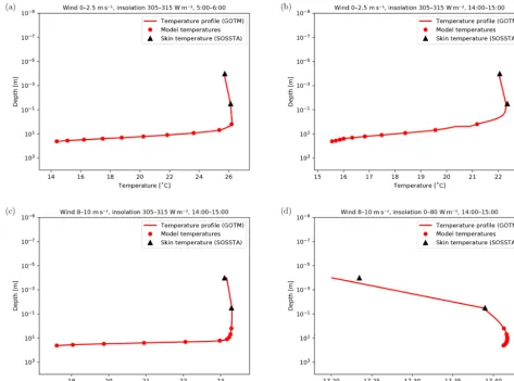
after-Figure 3.Examples of temperature profiles in various conditions and at different times. The GOTM profiles are shown by the red curve, while the filled circles indicate the values used as input to the CCA OO. The output of the CCA OO is shown by the black triangles.(a)Low wind, high insolation, early morning;(b)low wind, high insolation, afternoon;(c)high wind, high insolation, afternoon;(d)high wind, low insolation, afternoon.
noon profile on a similar day. At this time, diurnal warming is around its maximum, and the skin temperature has increased about 1◦C above the first level of the model. In the case of high wind speed, the increased mixing of the upper layer of the ocean can completely cancel the effect of the high inso-lation, as shown in Fig. 3c. In this situation the temperature in the upper 10 m of the ocean is almost constant. When high wind conditions coincide with low insolation, the surface can also cool quite significantly, as shown in Fig. 3d. The CCA OO is able to correctly reproduce the GOTM skin and sub-skin temperature under different atmospheric conditions. The atmospheric categories with strong diurnal warming have a root mean square error (RMSE) of up to 0.4◦C; for all other categories the RMSE is around 0.1◦C. The bias of the CCA OO compared to the GOTM was found to be negligible.
5 Performance and discussion
The performance of the GOTM-based CCA OO for SST is compared to other commonly used methods. For this com-parison the GOTM dataset is again split along the zonal di-rection using every other profile to calculate the CCA OO. The remaining profiles are matched to SEVIRI subskin re-trievals using only profiles matched to a measurement with an acceptable (4) or good (5) quality control level. The per-formance can be conveniently expressed in terms of the skill score (SS), defined by Murphy (1988) as
SS=1− MSEmodel MSEreference
. (15)
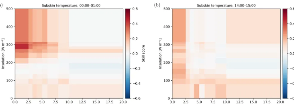
Figure 4.Skill score of the CCA OO compared to the OGCM upper layer for all wind and insolation categories at midnight(a)and in the afternoon(b).
1, while a model that shows no improvement over the refer-ence model receives a skill score of 0. Negative skill scores indicate that the model performs worse and its MSE has in-creased with respect to the reference. In this case the CCA OO will be used as the model and the reference will be an-other commonly used OO. The MSE is calculated with re-spect to the SEVIRI subskin temperature.
The simplest method of assimilating satellite SST observa-tions in a model that insufficiently describes the diurnal cycle of SST is to assimilate only at night or during high wind; see, for example, Waters et al. (2015). During the night the cycle of SST is close to its minimum value and the temperature of the upper layer of an OGCM forms a reasonable approxima-tion for the skin temperature. In this situaapproxima-tion the assimila-tion is performed without addiassimila-tional correcassimila-tions. Figure 4a shows the skill score of the CCA OO at midnight local time using the temperature of the OGCM upper layer as a refer-ence method. Figure 4b shows the same situation, but in the afternoon. For high wind and low insolation the CCA OO performs, as expected, similarly to using the upper OGCM layer. However, for low wind speeds and high insolation the CCA OO shows a clear improvement, even at midnight. This can be explained by the fact that at midnight some diurnal signal still remains and, even using the wind and insolation values of the next day, this is correctly modelled by the CCA OO.
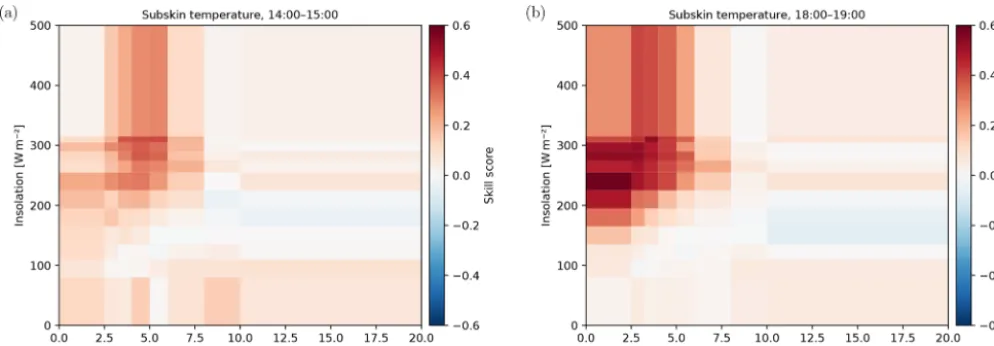
A more advanced solution is the parameterisation of Bernie et al. (2007), which estimates the diurnal signal as a function of wind, insolation, and time. This is a commonly used parameterisation; for example, it is included with the NEMO ocean model (Madec et al., 1998). Figure 5 shows the skill score for the CCA OO compared to the parameterisation of Bernie et al. (2007) at the peak of the diurnal cycle (a) and in the early evening (b). It can be seen that for high insolation and low wind, conditions for which the diurnal warming is
largest, both methods perform similarly. However, the CCA OO is better at accommodating different atmospheric condi-tions and shows significant improvements for the intermedi-ate insolation and wind cintermedi-ategories. Moreover, Fig. 5b shows that the CCA OO is able to better parameterise the cooling of the subskin in the late afternoon–evening after the peak of the diurnal warming has passed.
Using the CCA OO to improve the description of SST has many potential applications. For example, the CCA OO could be used as a parameterisation of diurnally varying skin SST within an OGCM as part of the air–sea flux calcula-tions. The skin SST is the true interface temperature for air– sea fluxes, so this approach should result in improved air– sea heat transfer in OGCMs and coupled ocean–atmosphere models. See, for example, Marullo et al. (2016). Another pos-sibility would be the use of the CCA OO as a parameterisa-tion of diurnally varying SST within a climate model. The di-urnal cycle is a fundamental signal of the climate system, yet for climate models the lack of vertical structure (and tempo-ral resolution) is even more critical. See, for example, Large and Caron (2015).
Due to the way in which it is constructed, the CCA OO is an inherently linear operator. This makes it straightforward to implement in DA schemes that require linearised and dif-ferentiable OOs. However, non-linear effects can be accom-modated to some extent by constructing a series of CCA OOs conditioned on such a non-linear dependency. For example, in the case of SST, this method has been used to condition the CCA OO on insolation, wind, and time. The only require-ment in this case is that the datasetsXandYof Sect. 3 are sufficiently large to divide them by such a dependent vari-able.
The minimum size of the input dataset required ultimately depends on the number of model variables used (Nx) and the
Figure 5.Skill score of the CCA OO compared to the parameterisation of Bernie et al. (2007) in the afternoon(a)and early evening(b).
of free parameters in the CCA OO matrixMand the offset Kequals(Nx+1)Ny. As each entry in the input dataset also
providesNyobservation values, Eq. (4) requires a minimum
ofNx+1 entries to be mathematically solvable. However, at
this point the CCA OO will be overfitted. It will simply be able to memorise the input datasets rather than being based on general characteristics of the data. Care has to be taken to avoid this situation, making sure the input dataset contains a number of entries n withn>>Nx. Whether a given size nis sufficient should be tested using independent data. One possible method for this test is to withhold part of the input dataset from the CCA OO calculation and then use this subset to calculate the CCA OO performance.
6 Conclusions
Observation operators (OOs) form a central component in any data assimilation (DA) system, as they transform the state variables of a numerical model into real-world observ-able variobserv-ables. Often, an OO also needs to correct for pro-cesses that are not fully described by the parent model. Such processes may be best modelled by interfacing the OO to a specialised model, but this is generally not feasible due to computational constraints.
The assimilation of satellite sea surface temperature (SST) in ocean general circulation models (OGCMs) is a prime ex-ample of a situation in which insufficiently modelled pro-cesses play an important role. The diurnal cycle of SST causes a discrepancy in the temperature of the very thin per layer measured by a satellite and the rather coarse up-per layer in a typical OGCM. On a clear summer day with low wind, this discrepancy can amount to as much as 2◦C or more (Pimentel et al., 2019).
The current paper presented a method, based on canonical correlation analysis (CCA), to build parameterisations based on an output dataset of a specialised model. These
parameter-isations, referred to as the CCA OO, can provide an efficient approximation to the results of the specialised model and are therefore well-suited for use in DA systems.
The case of SST assimilation has been used to demonstrate the new CCA OO. Using an output dataset of the General Ocean Turbulence Model (GOTM), a high-resolution wa-ter column model specifically tuned for modelling the diur-nal cycle of SST, a new CCA OO has been derived. Subse-quently, the operator has been applied to reduced-resolution temperature profiles from the GOTM to simulate its use in a DA system. The approximations provided by the CCA OO are found to be in good agreement with the GOTM at vari-ous times of the day and across all atmospheric conditions. The results indicate that the CCA OO could be used to en-able the assimilation of SST in conditions under which this was previously not possible. Moreover, the atmospheric cat-egories that were introduced in the construction of the CCA OO for SST show that the linear assumption implicit in CCA can be partially relaxed. This makes the CCA OO versatile for any condition. Compared to commonly used methods for SST assimilation, the CCA OO can provide substantial im-provements. This is especially true for measurements of the skin SST, since the CCA OO profits from the modelling of the cool-skin effect that is included in the GOTM.
Data availability. The GOTM dataset used in Sects. 4 and 5 is available as described in Pimentel et al. (2019). The code for cal-culating the CCA OO is available from the authors upon request.
Author contributions. EJ designed and implemented the CCA OO software. SP and WHT performed the modelling of the diurnal cy-cle. DD, GK, and IM evaluated the OO in different DA systems and provided feedback on the modelling and the software. AS was the PI of the project and coordinated the work. EJ prepared the paper with input from all co-authors.
Competing interests. The authors declare that they have no conflict of interest.
Special issue statement. This article is part of the special is-sue “The Copernicus Marine Environment Monitoring Service (CMEMS): scientific advances”. It is not associated with a confer-ence.
Acknowledgements. This work forms part of the SOSSTA project, which has been funded by the EU Copernicus Marine Environ-ment Monitoring Service (CMEMS) through the Service Evolution grants.
Review statement. This paper was edited by Pierre-Yves Le Traon and reviewed by Salvatore Marullo and one anonymous referee.
References
Bernie, D. J., Guilyardi, E., Madec, G., Slingo, J. M., and Wool-nough, S. J.: Impact of resolving the diurnal cycle in an ocean– atmosphere GCM. Part 1: a diurnally forced OGCM, Clim. Dy-nam., 29, 575–590, https://doi.org/10.1007/s00382-007-0249-6, 2007.
Björck, Å. and Golub, G. H.: Numerical Methods for Computing Angles Between Linear Subspaces, Math. Comput., 27, 579– 594, https://doi.org/10.2307/2005662, 1973.
Burchard, H., Bolding, K., and Ruiz-Villarreal, M.: GOTM, a gen-eral ocean turbulence model. Theory, implementation and test cases, Tech. Rep. EUR 18745 EN, European Commission, Brus-sels, Belgium, 1999.
Donlon, C. J., Minnett, P. J., Gentemann, C., Nightin-gale, T. J., Barton, I. J., Ward, B., and Murray, M. J.: Toward Improved Validation of Satellite Sea Surface Skin Temperature Measurements for Climate Research, J. Climate, 15, 353–369, https://doi.org/10.1175/1520-0442(2002)015<0353:TIVOSS>2.0.CO;2, 2002.
Flament, P., Firing, J., Sawyer, M., and Trefois, C.: Amplitude and Horizontal Structure of a Large Diurnal Sea Surface Warm-ing Event durWarm-ing the Coastal Ocean Dynamics Experiment, J. Phys. Oceanogr., 24, 124–139, https://doi.org/10.1175/1520-0485(1994)024<0124:AAHSOA>2.0.CO;2, 1994.
Haddad, Z. S., Steward, J. L., Tseng, H. C., Vukicevic, T., Chen, S. H., and Hristova-Veleva, S.: A data assimilation technique to account for the nonlinear dependence of scattering microwave observations of precipitation, J. Geophys. Res.-Atmos., 120, 5548–5563, https://doi.org/10.1002/2015JD023107, 2015. Harris, B. A. and Kelly, G.: A satellite radiance-bias correction
scheme for data assimilation, Q. J. Roy. Meteor. Soc., 127, 1453– 1468, https://doi.org/10.1002/qj.49712757418, 2001.
Hotelling, H.: Relations Between Two Sets of Variates, Biometrika, 28, 321–377, 1936.
Janji´c, T., Bormann, N., Bocquet, M., Carton, J. A., Cohn, S. E., Dance, S. L., Losa, S. N., Nichols, N. K., Potthast, R., Waller, J. A., and Weston, P.: On the representation error in data assimilation, Q. J. Roy. Meteor. Soc., 144, 1257–1278, https://doi.org/10.1002/qj.3130, 2018.
Large, W. G. and Caron, J. M.: Diurnal cycling of sea sur-face temperature, salinity, and current in the CESM coupled climate model, J. Geophys. Res.-Oceans, 120, 3711–3729, https://doi.org/10.1002/2014JC010691, 2015.
Madec, G., Delecluse, P., Imbard, M., and Lévy, C.: OPA 8.1 Ocean General Circulation Model Reference Model, Tech. Rep. 11, Institut Pierre Simon Laplace des Sciences de l’Environment Global, 1998.
Marullo, S., Santoleri, R., Ciani, D., Borgne, P. L., Péré, S., Pinardi, N., Tonani, M., and Nardone, G.: Combining model and geo-stationary satellite data to reconstruct hourly SST field over the Mediterranean Sea, Remote Sens. Environ., 146, 11–23, https://doi.org/10.1016/j.rse.2013.11.001, 2014.
Marullo, S., Minnett, P. J., Santoleri, R., and Tonani, M.: The diur-nal cycle of sea-surface temperature and estimation of the heat budget of the Mediterranean Sea, J. Geophys. Res.-Oceans, 121, 8351–8367, https://doi.org/10.1002/2016JC012192, 2016. Merchant, C. J., Filipiak, M. J., Le Borgne, P., Roquet, H., Autret,
E., Piollé, J. F., and Lavender, S.: Diurnal warm-layer events in the western Mediterranean and European shelf seas, Geophys. Res. Lett., 35, L04601, https://doi.org/10.1029/2007GL033071, 2008.
Murphy, A. H.: Skill Scores Based on the Mean Square Error and Their Relationships to the Correlation Coefficient, Mon. Weather Rev., 116, 2417–2424, https://doi.org/10.1175/1520-0493(1988)116<2417:SSBOTM>2.0.CO;2, 1988.
Oke, P. R. and Sakov, P.: Representation Error of Oceanic Observa-tions for Data Assimilation, J. Atmos. Ocean. Tech., 25, 1004– 1017, https://doi.org/10.1175/2007JTECHO558.1, 2008. Pimentel, S., Haines, K., and Nichols, N. K.: Modeling the diurnal
variability of sea surface temperatures, J. Geophys. Res.-Oceans, 113, C11004, https://doi.org/10.1029/2007JC004607, 2008a. Pimentel, S., Haines, K., and Nichols, N. K.: The
assimila-tion of satellite-derived sea surface temperatures into a di-urnal cycle model, J. Geophys. Res.-Oceans, 113, C09013, https://doi.org/10.1029/2007JC004608, 2008b.
Pimentel, S., Tse, W.-H., Xu, H., Denaxa, D., Jansen, E., Ko-rres, G., Mirouze, I., and Storto, A.: Modeling the near-surface diurnal cycle of sea near-surface temperature in the Mediterranean Sea, J. Geophys. Res.-Oceans, 124, 171–183, https://doi.org/10.1029/2018JC014289, 2019.
Saux Picart, S. and Legendre, G.: MSG/SEVIRI Sea Surface Temperature data record Product User Man-ual, Tech. Rep. OSI-250, EUMETSAT, OSI SAF, https://doi.org/10.15770/EUM_SAF_OSI_0004, 2018.
Simoncelli, S., Fratianni, C., Pinardi, N., Grandi, A., Drudi, M., Oddo, P., and Dobricic, S.: Mediterranean Sea phys-ical reanalysis (MEDREA 1987–2015) (Version 1), Tech. rep., EU Copernicus Marine Service Information, https://doi.org/10.25423/medsea_reanalysis_phys_006_004, 2014.
Umlauf, L., Burchard, H., and Bolding, K.: General Ocean Tur-bulence Model, Scientific Documentation v3.2., Tech. Rep. 63, Institute for Baltic Sea Research Warnemünde, Rostock-Warnemünde, Germany, 2005.