GREAT3 results – I. Systematic errors in shear estimation and the impact of real galaxy morphology

GREAT3 results – I. Systematic errors in shear estimation and the impact

of real galaxy morphology

Rachel Mandelbaum,

Barnaby Rowe,

Robert Armstrong,

Deborah Bard,

Emmanuel Bertin,

James Bosch,

Dominique Boutigny,

Frederic Courbin,

William A. Dawson,

Annamaria Donnarumma,

Ian Fenech Conti,

Rapha¨el Gavazzi,

Marc Gentile,

Mandeep S. S. Gill,

David W. Hogg,

Eric M. Huff,

M. James Jee,

Tomasz Kacprzak,

Martin Kilbinger,

Thibault Kuntzer,

Dustin Lang,

Wentao Luo,

Marisa C. March,

Philip J. Marshall,

Joshua E. Meyers,

Lance Miller,

Hironao Miyatake,

Reiko Nakajima,

Fred Maurice Ngol´e Mboula,

Guldariya Nurbaeva,

Yuki Okura,

St´ephane Paulin-Henriksson,

Jason Rhodes,

Michael D. Schneider,

Huanyuan Shan,

Erin S. Sheldon,

Melanie Simet,

Jean-Luc Starck,

Florent Sureau,

Malte Tewes,

Kristian Zarb Adami,

Jun Zhang

and Joe Zuntz

Affiliations are listed at the end of the paper

Accepted 2015 April 8. Received 2015 April 2; in original form 2014 December 4

A B S T R A C T

We present first results from the third GRavitational lEnsing Accuracy Testing (GREAT3) challenge, the third in a sequence of challenges for testing methods of inferring weak grav-itational lensing shear distortions from simulated galaxy images. GREAT3 was divided into experiments to test three specific questions, and included simulated space- and ground-based data with constant or cosmologically varying shear fields. The simplest (control) experiment included parametric galaxies with a realistic distribution of signal-to-noise, size, and elliptic-ity, and a complex point spread function (PSF). The other experiments tested the additional impact of realistic galaxy morphology, multiple exposure imaging, and the uncertainty about a spatially varying PSF; the last two questions will be explored in Paper II. The 24 participating teams competed to estimate lensing shears to within systematic error tolerances for upcoming Stage-IV dark energy surveys, making 1525 submissions overall. GREAT3 saw considerable variety and innovation in the types of methods applied. Several teams now meet or exceed the targets in many of the tests conducted (to within the statistical errors). We conclude that the presence of realistic galaxy morphology in simulations changes shear calibration biases by

∼1 per cent for a wide range of methods. Other effects such as truncation biases due to finite galaxy postage stamps, and the impact of galaxy type as measured by the S´ersic index, are quantified for the first time. Our results generalize previous studies regarding sensitivities to galaxy size and signal-to-noise, and to PSF properties such as seeing and defocus. Almost all methods’ results support the simple model in which additive shear biases depend linearly on PSF ellipticity.

Key words: gravitational lensing: weak – methods: data analysis – techniques: image processing – cosmology: observations.

_{E-mail:[email protected](RM);[email protected](BR)} 2015 The Authors

at California Institute of Technology on July 9, 2015

http://mnras.oxfordjournals.org/

1 I N T R O D U C T I O N

Weak gravitational lensing, the small but coherent deflections of light from distant objects due to the gravitational field of more nearby matter (for a review, see Bartelmann & Schneider2001; Refregier2003; Schneider2006; Hoekstra & Jain2008; Massey, Kitching & Richard2010), has emerged in the past two decades as a promising way to constrain cosmological models, to study the relationship between visible and dark matter, and even to constrain the theory of gravity on cosmological scales (e.g. Hu2002; Huterer 2002; Abazajian & Dodelson2003; Zhang et al.2007). Because of this promise, gravitational lensing has already been measured in many data sets, and there are several large surveys planned for the next few decades to measure weak lensing even more precisely,

including Euclid1 _{(Laureijs et al. 2011), LSST}2 _{(LSST Science}

Collaborations et al.2009), and WFIRST-AFTA3_{(Spergel et al.}

2013), all of which are Stage IV dark energy experiments according to the Dark Energy Task Force (Albrecht et al.2006) definitions.

The most common type of weak lensing measurement involves measuring coherent distortions (‘shear’) in the shapes of galaxies. In order for the aforementioned surveys to make the most of their ability to measure these distortions with sub-per cent statistical er-rors, they must ensure adequate control of systematic errors. While a full systematic error budget for weak lensing includes both as-trophysical and instrumental systematic errors, a problem that has occupied much attention in the community for over a decade is ensuring accurate measurements of the shear distortions of galaxies given that they have been convolved with a point spread function (PSF) and rendered into noisy images.

With the rapid proliferation of shear estimation methods, the weak lensing community began a series of blind community chal-lenges, with simulations that included a lensing shear (known only to the organizers) that participants must measure. This served as a way to benchmark different shear estimation methods. The ear-liest of these challenges were the first Shear TEsting Programme

(STEP1; Heymans et al.2006) and its successor (STEP2; Massey

et al.2007a). Then, it became apparent that many complex aspects of the process of shear estimation would benefit from simpler and more controlled simulations, which led to the GRavitational lEnsing Accuracy Testing (GREAT08) challenge (Bridle et al.2009,2010),

followed by the GREAT10 challenge (Kitching et al.2010,2012,

2013).

Each of these challenges has been informative in its own way, illuminating important issues in shear estimation while also gener-ating significant improvement in the accuracy of weak lensing shear estimation. For example, both the GREAT08 and GREAT10 chal-lenges highlighted the role played by pixel noise in biasing shear es-timates. While this signal-to-noise (S/N)- and resolution-dependent ‘noise bias’ was studied in specific contexts before GREAT08 and GREAT10 (e.g. Bernstein & Jarvis2002; Hirata et al.2004), the landscape changed after GREAT08, with several more general stud-ies (Kacprzak et al.2012; Melchior & Viola2012; Refregier et al. 2012), some of which used the GREAT10 simulations as a test for calibration schemes. However, despite the progress encouraged by these challenges, there remained a number of outstanding issues in shear estimation that needed to be addressed for the commu-nity to ensure its ability to measure weak lensing in near-term and future surveys. These issues include the impact of realistic galaxy

1_{http://sci.esa.int/euclid/,http://www.euclid-ec.org} 2_{http://www.lsst.org/lsst/}

3_{http://wfirst.gsfc.nasa.gov}

morphology; a number of studies have convincingly demonstrated that when estimating shears in a way that assumes a particular galaxy model, the shears can be biased if the galaxy light profiles are not correctly described by that model (termed ‘model bias’; Melchior et al.2010; Voigt & Bridle2010). More generally, any method based on the use of second moments to estimate shears cannot be completely independent of the details of the galaxy light profiles, such as the overall galaxy morphology and presence of de-tailed substructure (Massey et al.2007b; Bernstein2010; Zhang & Komatsu2011). Thus, the question of the impact of realistic galaxy morphology (and the way that galaxies deviate from simple para-metric models) on shear estimation is important to address in a community-wide challenge. This is one of the key questions of the GREAT3 challenge.

The GREAT3 challenge was also designed to address two ad-ditional questions. One of these is the combination of multiple exposures, which is necessary to analyse the data from nearly any current or upcoming weak lensing survey. For Nyquist-sampled data this is relatively straightforward, but for data that are not Nyquist-sampled (such as some images from space telescopes), the problem is more challenging (e.g. Lauer1999; Fruchter2011; Rowe, Hirata & Rhodes2011). The final problem addressed in GREAT3 is the impact of PSF estimation from stars and interpolation to the posi-tions of the galaxies. However, this paper will focus predominantly on the question of shear estimation in general and realistic galaxy morphology in particular, leaving the other questions for Paper II.

In Section 2, we describe how the challenge was designed and run, how submissions were evaluated, and a basic summary of the submissions that were made. We discuss the methods used by participants to analyse the simulated data in Section 3. For certain methods for which the teams made many submissions, we derive lessons related to those methods in Section 4. We then present the overall results for all teams in Section 5. Section 6 describes some lessons learned about shear estimation from GREAT3, and we conclude in Section 7. Finally, there are appendices with some further technical details related to the challenge simulations, and lengthier descriptions of the methods used by each team.

2 T H E C H A L L E N G E 2.1 Theoretical background

Gravitational lensing distorts the images of distant galaxies. When this distortion can be described as a locally linear transformation, then the lensing effect is described as ‘weak’. In this case, it relates unlensed coordinates (xu,yu; with the origin at the centre of the

distant light source) and the observed, lensed coordinates (xl, yl;

with the origin at the centre of the observed image), via

xu yu = 1−γ1−κ −γ2 −γ2 1+γ1−κ xl yl . (1)

The two components of the lensing shear (γ1, γ2) describe the

stretching of galaxy images due to lensing, whereas the convergence

κ describes a change in apparent size and brightness for lensed

objects. This transformation is often recast as

xu yu =(1−κ) 1−g1 −g2 −g2 1+g1 xl yl , (2)

in terms of the reduced shear, gi = γi/(1 − κ) γi in most

cosmological applications. Typically, it is the stretching described by the reduced shear that is actually observed. We often encode

at California Institute of Technology on July 9, 2015

http://mnras.oxfordjournals.org/

the two components of shear (reduced shear) as a single complex number,γ=γ1+iγ2(g=g1+ig2).

The lensing shear causes a change in estimates of theellipticity of distant galaxies. In practice, the effect is estimated statistically by measuring galaxy properties that transform in simple ways under a shear. One method is to model the galaxy image using a profile with a well-defined ellipticity, written asε=ε1+iε2, with magnitude

|ε| = 1−b/a

1+b/a (3)

for semiminor and semimajor axis lengthsbanda, and orientation angle determined by the major axis direction. For a population of randomly oriented source intrinsic ellipticities, the ensemble average ellipticity after lensing gives an unbiased estimate of the

shear:ε g.

Another common choice of shape parametrization is based on second brightness moments of the galaxy image,

Qij =

d2xI(x)W(x)xixj

d2_xI(x)W(x) , (4)

where (x1,x2) correspond to the (x,y) directions,I(x) denotes the

galaxy image light profile,W(x) is an optional4_{weight function}

(see e.g. Schneider2006), and the coordinate origin is placed at the galaxy image centre. A second ellipticity definition (sometimes called thedistortionto distinguish it from the ellipticity that satisfies equation 3) can be written as

e=e1+ie2=

Q11−Q22+2iQ12

Q11+Q22

. (5)

The ellipticityεcan also be related to the moments by replacing the denominator in equation (5) withQ11+Q22+2(Q11Q22−

Q2 12)

1/2_.

If the weight functionWis constant or brightness-dependent, an image with elliptical isophotes has

|e| =1−b2/a2

1+b2/a2. (6)

For a randomly oriented population of source distortions, the en-semble averageeafter lensing gives an unbiased estimate of shear that depends on the population root mean square (rms) distortion (e(s)₎2_{ase 2[1− (e}(s)₎2_]g.

See e.g. Bernstein & Jarvis (2002) for further details on com-monly used shear and ellipticity definitions.

2.2 Summary of challenge structure

Here, we describe how the GREAT3 challenge was structured; more details are given in the handbook (Mandelbaum et al.2014).

The GREAT3 challenge was designed to address how three issues affect shear estimation: (a) the impact of realistic galaxy morphol-ogy, (b) the impact of the image combination process, and (c) the effect of errors due to estimation and interpolation of the PSF. To this end, the challenge consisted of five experiments.

(1) Control: parametric (single or double S´ersic) galaxy models based on fits (Lackner & Gunn2012) toHubble Space Telescope

(HST) data from the COSMOS (Koekemoer et al.2007; Scoville

et al.2007a,b) survey, meant to represent the galaxy population

4_{Optional for the purpose of this definition; but in practice, for images with} noise, some weight function that reduces the contribution from the wings of the galaxy is necessary to avoid moments being dominated by noise.

in a typical weak lensing survey, including appropriate size versus galaxy flux S/N relations, morphology distributions, and so on. In each image, the non-trivially complex PSF was provided for the participants as a set of nine images with different centroid offsets.

(2) Real galaxy: differed from the control experiment only in the

use of the actual images from theHSTCOSMOS data set instead

of the best-fitting parametric models.

(3) Multiepoch: differed from the control experiment only in that each field contained six images (representing observations that must be combined) instead of one. For the space branches, the six images were not Nyquist sampled.

(4) Variable PSF: differed from the control experiment only in that the PSF varied across the image in a realistic way, and had to be estimated from star images.

(5) Full: included the complications of the real galaxy, multi-epoch, and variable PSF experiments all together.

In all cases, the goal was to estimate the lensing shear.5_{For each}

experiment, there were four branches, which came from the combi-nation of two types of simulated data (ground, space) and two types of shear fields (constant, variable). For convenience, we will refer to branches by their combinations of{experiment}–{observation type}–{shear type}, e.g. control–ground–constant, and will use the unique abbreviations CGC, CGV, and so on. Of the 20 branches

(five experiments ×two data types×two shear types),

partici-pants could submit results for as many or few as they chose (see Mandelbaum et al.2014, Fig.5). A given branch included 200 sub-fields, each with 104_{galaxies on grids. To reduce statistical errors}

on the shear biases, galaxies were arranged such that the intrinsic noise due to non-circular galaxy shapes (‘shape noise’) was nearly cancelled out.

Submissions to the challenge were evaluated according to met-rics described in Section 2.3. Within a branch, teams were ranked based on their best submission in that branch. Per-branch rankings were used to award teams points, which were then added up across multiple branches to give an overall leaderboard ranking. While the leaderboard ranking was necessary for the purpose of carrying out a challenge, the goal of this work is to study how teams performed and derive lessons for the future based on analysis that goes far beyond a simple ranking scheme.

There are a number of online resources related to the challenge and the simulations. The main challenge web site6_contains

over-all information. The leaderboard web site, linked from the main challenge web site, contains the archived challenge leaderboards, and additional post-challenge boards to which submissions were made after the end of the challenge. It also links to download the

GREAT3 simulations and truth tables. The GitHub site7_contains

software to reproduce the simulated data and to analyse it using simple methods, and a wiki with information for the participants. Finally,GALSIM8is the simulation software that was used to make the

GREAT3 simulations, and its algorithms, design, and functionality are described in Rowe et al. (2015).

Some physical effects that are not tested in the challenge include object detection, selection, and deblending, because the galaxies are located on grids; wavelength-dependent effects; instrumental

5_{This is not the same as testing the ability to measure a per-galaxyshape.} Two different methods can recover a different per-galaxy shape, while still estimating the overall shear accurately.

6_{http://www.great3challenge.info}

7_{https://github.com/barnabytprowe/great3-public} 8_{https://github.com/GalSim-developers/GalSim}

at California Institute of Technology on July 9, 2015

http://mnras.oxfordjournals.org/

and detector defects or non-linearities; star/galaxy separation; back-ground estimation; complex pixel noise models; cosmic rays and other image artefacts; redshift-dependent shear calibration; shear estimation for galaxies with sizes comparable to the PSF; non-weak shear signals (e.g. cluster lensing); and flexion.

Appendix A contains more detailed information about some as-pects of the challenge that were not in the handbook. These in-clude Appendix A1, on the intrinsic ellipticity distribution (p(ε)) of the galaxies; Appendix A2, which describes the distributions from which the lensing shears were drawn; Appendix A3, which presents distributions of optical and atmospheric PSF properties; and Appendix A4, which shows the actual S/N distributions for galaxies in GREAT3. The last point is particularly relevant for how pixel noise should affect shear estimates in the challenge.

Finally, the GREAT3 Executive Committee9_{(EC) distributed}

ex-ample scripts to automatically process the challenge data, including shear estimation, co-addition of multi-epoch data, and variable PSF estimation. While the latter two will be discussed in Paper II, we describe the algorithms in the shear estimation example script in Appendix B.

2.3 Diagnostics

Here, we describe the diagnostics used to quantify the performance of each submission to the challenge. The metrics for constant- and variable-shear branches, discussed in detail in Mandelbaum et al. (2014), were used to rank submissions. Here, we briefly define the equations used.

2.3.1 Constant shear

For constant-shear simulations, each field has a particular value of shear applied to all galaxies (Appendix A2). Participants submitted estimated (‘observed’) shears for each constant shear value in the branch. We relate biases in observed shearsgobs_{to the true shear}

gtrue_{using a linear model in each component,}

gobs

i −gtruei =migitrue+ci, (7)

whereidenotes the shear component, andmiandciare the

mul-tiplicative and additive biases, respectively. From user-submitted estimates of allgobs

i in a branch, the metric calculation begins with an unweighted least-squares linear regression to provide estimates ofmi,cigiven the true shears (in Section 4.8, we discuss the role

of outliers in affecting themiandciestimates). The regression is

done in a coordinate frame rotated to be aligned with the mean PSF ellipticity in each field, so thatcvalues will properly reflect the contamination of galaxy shapes by the PSF anisotropy.

Having estimatedmiandci, we constructed the metric,Qc, by

comparison with ‘target’ values mtarget, ctarget. These come from

requirements for upcoming weak lensing experiments; we use mtarget = 2× 10−3 and ctarget = 2× 10−4, motivated by a

re-cent estimate of requirements (Cropper et al.2013; Massey et al.

9_{The EC created the simulations, ranking scheme, and other aspects of the} challenge, and had access to privileged information about the simulations. Because of this access, teams to which they made significant contributions did not receive points in the challenge, and were not ranked. Those teams appear on the leaderboard with an asterisk for their score.

2013) for theEuclidspace mission. The constant-shear metric is then defined as Qc= 2000×ηc σ2 min,c+ i=+,× mi mtarget 2 + _c i ctarget 2 . (8)

The indices+,×refer to the two shear components in the rotated reference frame described above. We adoptσ2

min,c=1(4) for space

(ground) branches, corresponding to the typical dispersion in the quadrature sum ofmi/mtargetandci/ctargetdue to pixel noise. This

metric is normalized byηcsuch that methods that meet our chosen

targets onmiandciin space-based data should achieveQc1000.

In the ground branchesQcis slightly lower for submissions

reach-ing target bias levels, reflectreach-ing their largerσ2

min,c due to greater

uncertainty in individual shear estimates for ground data. However, Qcscores are consistent between space and ground branches where

biases are significant.

Given the nature of this metric definition, the uncertainty inQc

is larger at highQcthan at smallQc. For the level of pixel noise

in the simulations from ground (space), the effective uncertainty on QcforQcvalues of [100, 300, 500, 1000] is [3, 28, 80, 328] ([2, 19,

55, 229]).

2.3.2 Variable shear

For variable-shear simulations, the key test is the reconstruction of the shear correlation function. Submission of results for these branches begins with calculation of correlation functions by the participant.10_{The submission consists of estimates of the aperture}

mass dispersion (e.g. Schneider et al.1998; Schneider2006), which are constructed from two-point correlation function estimates, and allows a separation into contributions fromEandBmodes.11_We

label theseEandBmode aperture mass dispersionsMEandMB.

The submissions were estimates of ME,j for each of 10 fields

labelled by indexj; this estimate is constructed using 20 subfields in a given field. This choice provides a large dynamic range of spatial scales in the correlation function, and thereby probes a greater range of shear signals. TheME,j are estimated inNbins logarithmically

spaced annular bins of galaxy pair separationθk, from the smallest

available angular scales in the field to the largest.

The metricQvfor the variable-shear branches was constructed by

comparison to the known, true value of the aperture mass dispersion for the realization ofE-mode shears in each field. These we label ME, true,j(θk). The variable-shear branch metric is then calculated as

Qv= 1000×ηv σ2 min,v+ 1 Nnorm Nbins k=1 Nfields j=1 ME,j(θk)−ME,true,j(θk) , (9)

whereNnorm=NfieldsNbins,σmin2 ,v=4(9)×10−

8_{for space (ground)}

branches, andηvis a normalization factor designed to yieldQv

1000 for a method achievingm1=m2=mtargetandc1=c2=ctarget.

The primary source of noise in theME,j(θk) is pixel noise, with

some residual shape noise playing a role despite the shape noise cancellation scheme. After the end of the challenge, we found that a

10_{Software for this purpose was distributed publicly at https://github.}

com/barnabytprowe/great3-public

11_{For more discussion of the limitations onE- andB-mode separation in} GREAT3, please see Mandelbaum et al. (2014).

at California Institute of Technology on July 9, 2015

http://mnras.oxfordjournals.org/

small additional source of noise comes from the interplay between theθkbin size, the galaxy grid configuration, and approximations

used in the calculation of the correlation function and aperture mass dispersion inCORR2.12While this is a subdominant source of

noise (∼1/4 of that due to measurement error), it does mean that participants will find that theirQvresults depend slightly on the

ordering of galaxies in their catalogue.

For the level of pixel noise in the simulations from ground (space), the effective uncertainty onQvforQvvalues of [100, 300, 500, 1000]

is [6, 47, 118, 418] ([5, 36, 91, 326]).

2.3.3 Other diagnostics

For the constant-shear branches, we have a clean way to directly study additive and multiplicative biases in the form ofmiandci,

wherei= +,×(defined in the frame aligned with the PSF ellipticity, and at 45◦ angles with respect to that direction). However, also of interest are themi andcidefined in the frame defined by the

pixel coordinates, fori=1, 2. In the STEP2 challenge (Massey

et al.2007a), many methods exhibited coherent differences in shear systematics along the pixel axes and at 45◦with respect to them, presumably due to the different effective sampling of the galaxy and PSF profiles. Since the PSF ellipticity direction has a random orientation with respect to the pixel axes, differences betweenm1

andm2will average out, givingm+≈m×. Since differences between

m1andm2may be interesting in understanding the performance of

a method, we will usem1andm2for some of our plots.

In addition,c1andc2may be of interest. Whilec+shows the

influ-ence of PSF anisotropy, additive systematics due to PSF anisotropy will have a random sign and direction for each subfield in the pixel coordinate frame, soc1andc2have an expectation value of zero.

Non-zero values may indicate selection biases with respect to the pixel direction, or asymmetric numerical artefacts.

Given the more fundamental nature ofm1andm2, and the need

to usec₊ to identify additive PSF systematics, we also consider what we will call a ‘mixed metric’,Qmix, defined in analogy toQc

(equation 8) as Qmix= 2000×ηc σ2 min,c+ i=1,2 _m i mtarget 2 + i=+,× _c i ctarget 2. (10) 2.4 Challenge process

During the challenge period, there were 1525 submissions13_with

non-zero score, from 24 distinct teams. Of these, two teams were actually members of the GREAT3 EC making submissions based on simple test scripts to validate the simulations or submission process; 16 were teams of participants; and 6 were teams that included at least one member of the GREAT3 EC, and were thus excluded from winning any points or the challenge itself.

Fig.1shows the number of submissions to the challenge as a

function of time, expressed in terms of weeks until the deadline. The first entries were submitted near the beginning of the challenge period, which ran from 2013 mid-October until 2014 April 30. The submission rate was an increasing function of time particularly in

12_{https://code.google.com/p/mjarvis/}

13_{The leaderboard website shows 1532 submissions, but seven had an} in-correct submission format, givingQ=0.

Figure 1. Number of submissions to the GREAT3 challenge as a function of time, expressed in terms of weeks until the deadline. The rules for the number of submissions per team per day were relaxed in the final week of the challenge.

Table 1. For each branch, this table shows the winning team and its score, the number of teams that submitted to that branch (with the number having scores above 500 for the submissions analysed in Section 5 shown in parenthesis), and the total number of entries in the branch.

Branch Winning Winning No. of No. of

team score teams entries

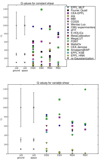
CGC CEA-EPFL 1211 22 (4) 250 CGV CEA-EPFL 1068 16 (5) 160 CSC Amalgam@IAP 1516 16 (3) 110 CSV Amalgam@IAP 1199 11 (4) 96 RGC Amalgam@IAP 1121 20 (4) 195 RGV CEA-EPFL 791 14 (4) 93 RSC Fourier_Quad 1919 12 (3) 92 RSV MegaLUT 1667 9 (4) 83 MGC sFIT 1017 9 (3) 71 MGV MegaLUT 1131 7 (2) 53 MSC sFIT 841 6 (1) 48 MSV CEA-EPFL 1605 6 (5) 45 VGC sFIT 884 7 (1) 60 VGV Amalgam@IAP 230 6 (0) 60 VSC Amalgam@IAP 1183 4 (1) 25 VSV sFIT 1276 4 (2) 17 FGC sFIT 800 2 (1) 11 FGV sFIT 379 2 (0) 17 FSC sFIT 1184 2 (2) 17 FSV sFIT 856 2 (2) 25

the last month; the spike in entries in the last week was partly due to a relaxation of the rules on the number of entries per team per day.

Two teams entered all 20 branches, and 7/24 (30 per cent) of the teams entered more than half the branches. Not surprisingly, many teams chose to focus on the control and realistic galaxy branches, which required the least amount of software infrastructure to par-ticipate.

Table1shows the results for each branch, including the winning team, the winning score (defined in Section 2.3), the number of participating teams, and the number of entries. As shown, a variety of teams with different methods won individual branches, rather than one team dominating everything. For all but two branches,

VGV and FGV, the winning scores were800, meaning that within

at California Institute of Technology on July 9, 2015

http://mnras.oxfordjournals.org/

Figure 2. Qfor all submissions as a function of time, expressed in terms of weeks until the deadline. Later submissions by the same team that appear to perform worse than earlier submissions typically went to more challenging branches.

the ability of the simulations to determine shear systematic errors, the winning submissions were effectively unbiased. Not only the winning team but also typically several other teams had scores in this range, representing an unprecedented quality of submissions in a weak lensing community challenge. We will discuss why the combination of variable PSF and variable shear was more difficult in Paper II.

To motivate the approach, we take for the analysis, Fig.2shows a scatter plot of metricQ(eitherQcorQvas appropriate) as a function

of time, for all submissions across all branches. Point styles indicate the team; the legend has been suppressed because our purpose is only to show that (1) there are a huge number of submissions with a wide range of performance, and (2) sometimes even within a given team, the results varied a great deal. We thus approach the analysis in two stages. Our first step, in Section 4, is to analyse the results for specific teams that made many submissions, to understand the trends for that method and identify a fair subset of their submissions (one per branch) to compare with those from other teams. Then, in Section 5, we use this fair subsample of submissions, one per team per branch, to learn lessons from the overall challenge results.

3 S H E A R E S T I M AT I O N M E T H O D S

In this section, we broadly categorize and describe the methods used to analyse the GREAT3 data. Appendix C contains a more detailed description of all methods. The main aspects of the methods used

by the teams in GREAT3 are summarized in Table2, which forms

the basis for the discussion in this section.14

We have assigned each of the 21 teams to a ‘class’ (listed in Table2) that describes how the method essentially works. There are several options for the class.

14_{A few teams listed on the GREAT3 challenge web site are not in this} table, either because they did not make any submissions, because the team solely existed to demonstrate the use of the example scripts (Appendix B) distributed by the GREAT3 EC (team ‘GREAT3_EC’), or because the team was created by a GREAT3 EC member only to check the GREAT3 simula-tions as part of the validation process (team ‘miyatake-test’).

(1) Maximum likelihood: maximum-likelihood model-fitting methods, of which there are five.

(2) Bayesian methods: there are four of these, each with different labels (e.g. ‘Bayesian hierarchical’, ‘Bayesian Fourier’, etc.) indi-cating differences in how they work. The ‘Partially Bayesian’ label for MaltaOx is meant to indicate a Bayesian marginalization over nuisance parameters combined with mean likelihood estimation, rather than a fully Bayesian approach.

(3) Moments: there are eight methods that work by combining estimates of galaxy and PSF moments in some way. Of these, six are real-space moments methods (called ‘Moments’) and two are Fourier-space moments methods (‘Fourier moments’). Of the six real-space moments methods, one involves as a key aspect of the method a self-calibration scheme (‘Moments+self-calibration’), and that self-calibration could be extended to non-moments-based methods.

(4) Stacking: a single team used image stacking.

(5) Neural network and supervised machine learning (ML): three methods rely heavily on ML.

The table also lists the weighting scheme that was used. Here, there are a few options. Several teams used constant (equal) weighting, in some cases allowing optional rejection using certain selection criteria (‘Constant+rejection’). Many teams used inverse variance weighting, where the variance is a combination of shape noise and measurement error due to pixel noise. In the Bayesian methods, the weights are often implicit rather than explicitly assigned. Some teams experimented with multiple weighting schemes, in which case their entry in the table is ‘Various’, and details are in the appendix.

Another important entry in Table2is ‘Calibration philosophy’, which relates to how or whether a team tries to calibrate out sys-tematic errors, versus attempting to be unbiased a priori. Here there are a few options.

(a) None: these teams apply no calibration corrections. (b) External simulations: these teams generate their own simula-tions in order to calibrate their shears. In one case (sFIT), these are produced iteratively until they are found to sufficiently match the data that are being analysed [‘External simulations (iterative)’].

(c) Ellipticity penalty term: one team, rather than applying cal-ibrations after the fact, uses a penalty term on high ellipticity to reduce certain calibration biases. This penalty term must be cali-brated in some way, making it somewhat different in nature from the next option.

(d)p(ε) from deep data: some methods require an input intrin-sic ellipticity distribution from deep data (or more precisely, for BAMPenn, the full distribution of unnormalized moments). This is qualitatively different from requiring external simulations, since many surveys will have a deeper subset of the data that could be used to derive this prior.

(e) Inferredp(ε): one team tried to hierarchically infer thep(ε) and the shear from the data itself.

(f) Self-calibration: finally, two teams (MetaCalibration and Mal-taOx) implemented a self-calibration scheme to derive calibration corrections from the data itself.

Table2also lists other useful pieces of information about these methods, as described in the caption.

at California Institute of Technology on July 9, 2015

http://mnras.oxfordjournals.org/

Table 2. Table summarizing the methods used by teams that participated in the challenge, including basic information such as team name; class (overall type of method); weighting scheme; calibration philosophy (discussed in the text); and number of branches entered in the challenge (Nbranch). ‘Limitations’ refers to types of data to which the implementation used here is not applicable without significant further development. ‘Rank’ is the leaderboard ranking for those that received points (‘-’ for those that did not, and ‘N/A’ for those that were ineligible due to participation of a GREAT3 EC member). ‘exact PSF?’ indicates whether they used the exact PSF or an approximation to it (e.g. sums of Gaussians). ‘New software’ indicates whether the software used to analyse the GREAT3 simulations was newly developed (‘yes’), included some existing infrastructure with new software of non-trivial complexity (‘some’), or was entirely pre-existing (‘no’). Finally, we show the approximate processing time per galaxy per exposure (on a single core) for science-quality shear estimates. Several fields are discussed in detail in Section 3.

Team Class Weighting Calibration Limitations Nbranch Rank Exact New Time per

scheme philosophy PSF? software galaxy

Amalgam@IAP Maximum Inverse Ellipticity None 16 2 Yes Some 0.1–1 s

likelihood variance penalty

BAMPenn Bayesian Implicit p(ε) from Variable 2 - Yes Yes <1 s

Fourier deep data shear

EPFL_gfit Maximum Constant+ None None 8 6 Yes Yes 1–3 s

likelihood rejection

CEA-EPFL Maximum Various None None 20 3 Yes Yes 1–3 s

likelihood

CEA_denoise Moments Constant None None 8 - Yes No 0.03 s

CMU Stacking Constant External Variable 2 N/A Yes Some 0.03 s

experimenters simulations shear

COGS Maximum Constant External None 12 N/A Yes Yes 1 s

(IM3SHAPE) likelihood simulations

E-HOLICS Moments Constant+ External None 12 8 Yes No 1–3 s

rejection simulations

EPFL_HNN Neural Constant None None 7 - Yes Yes 2–3 s

network

EPFL_KSB Moments Inverse None None 4 - Yes No 0.001–0.002 s

variance

EPFL_MLP / Neural Constant None None 5 - Yes Yes 2–3 s

EPFL_MLP_FIT network

FDNT Fourier Inverse External None 12 N/A Yes Some ∼1 s

moments variance simulations

Fourier_Quad Fourier Various None None 6 5 Yes No 0.001–0.002 s

moments

HSC/LSST-HSM Moments Inverse External None 4 N/A Yes Some 0.05 s

variance simulations

MBI Bayesian Implicit Inferred Variable 4 9 No Some 10 s

hierarchical p(ε) shear, PSF

MaltaOx Partially Inverse Self- None 3 7 Yes Some 0.05 s

(LENSFIT) Bayesian variance calibration

MegaLUT Supervised Constant+ External None 16 4 Yes Some 0.02 s

ML rejection simulations

MetaCalibration Moments+ Inverse Self- Variable 1 N/A Yes Yes 0.3 s

self-calibration variance calibration shear

Wentao_Luo Moments Inverse None None 4 - Yes Yes 1–2 s

variance

ess Bayesian Implicit p(ε) from Variable 2 - No Yes 1 s

model-fitting deep data shear

sFIT Maximum Inverse External None 20 1 Yes Yes 0.8 s

likelihood variance simulations (iterative)

at California Institute of Technology on July 9, 2015

http://mnras.oxfordjournals.org/

4 I N F O R M AT I V E R E S U LT S F O R S P E C I F I C M E T H O D S

Before exploring the overall results of the challenge, we first con-sider several methods in detail. For methods with many submissions, it is important to understand overall behaviour of the method before comparing with others. For this reason, we carry out two types of tests.

(1) Controlled tests of the performance of the method as a func-tion of the various initial settings and parameter values that deter-mine its performance, for multiple submissionsin a given branch.

(2) A comparison of submissions for that methodacross multiple branches, while holding its initial settings and parameters fixed (instead of using those that happened to give the best metric score in each branch).

These results then serve as a basis for the fair comparison between methods and across branches, which will be performed later in the paper. For all the methods discussed, see Appendix C for a more detailed description.

4.1 GFIT

4.1.1 Controlled tests of variation inGFITparameters

In this section, we show results of a more detailed exploration of theGFITsoftware used by the EPFL_GFITand CEA-EPFL teams (see

method descriptions in Appendices C3 and C4). In particular, we investigate the dependence of the results on choices made in the course of estimating the per-object shears, or the weighting used to estimate an average shear for the entire field. Our comparison focuses on the constant-shear branches, where we have additional diagnostics such as the multiplicative and additive biases (see Sec-tion 2.3 for definiSec-tions).

This comparison uses the submissions from EPFL_GFIT, but the

results are also applicable to CEA-EPFL submissions. The factors that were considered in the comparison are the galaxy model, the postage stamp size, precision on the total flux and centroid, max-imum half-light radii of the bulge and disc, filtering of the galaxy catalogue, constraints on positivity of bulge and disc flux, and oc-casional other experiments, such as stacking the nine PSFs in the starfield images, or running a denoising scheme.

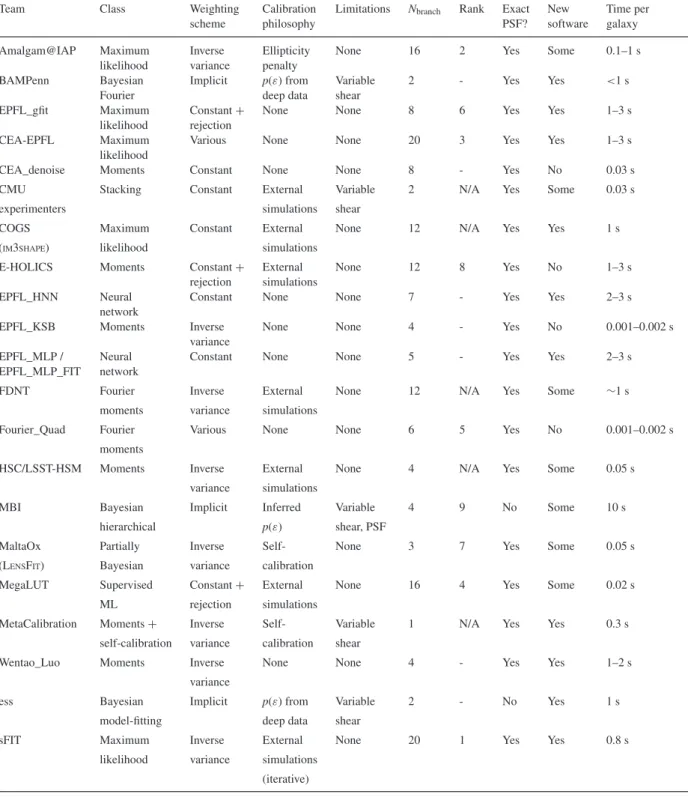
We begin by analysing the 14 submissions in RGC. Correlating theQcvalues with the settings that vary for these submissions, we

find that the parameter that most directly predictsQcis the postage

stamp size used for the model fitting (see top panel of Fig.3). As

shown, using the full 48 ×48 postage stamp maximizes theQc

score.

To understand this correlation, we consider the multiplicative bias as a function of postage stamp size (middle panel of Fig.3). As shown, except for a few outliers, the multiplicative biasesm₊and m_×that contribute toQcincrease from being consistent with zero to

2.0±0.4 and 2.2±0.5 per cent, respectively, as the postage stamp is reduced to half of its (linear) size. The statistical significance of the difference between the results with the maximum and minimum stamp size is more than the 3σ that it appears to be in Fig.3; given the high (∼0.75) correlation coefficient between the submissions, the change inmis detected at approximately 8σsignificance.

For maximum-likelihood fitting methods, we expect a calibration bias due to the effects of noise (‘noise bias’). One interpretation of the RGC results at the maximal postage stamp size is therefore a

Figure 3. QcandQmix(top), and the bias componentsmi(middle) andci

(bottom), for theGFITmethod as a function of the postage stamp size used for modelling the galaxy images in the RGC branch. The target regions are shown as a grey shaded region, within which the vertical axis has a linear scaling; outside of the shaded region, the scaling is logarithmic. Multiple submissions with the same stamp size have slight horizontal offsets for clarity. The error bars are correlated between the submissions, so the figure cannot be used to assess statistical significance of differences between them. See the discussion in the text for quantitative calculations of statistical significance. Themi andcipanels only show errors on a single quantity

(i= +), for clarity.

at California Institute of Technology on July 9, 2015

http://mnras.oxfordjournals.org/

(cancelling) combination of noise bias with other potential biases, such as those expected due to an imperfect galaxy model.

As the postage stamp size is reduced, the likelihood surface for the shear estimate changes due to reduced information about the light profile, and this change will generally depend on the galaxy size and shape, postage stamp size, and the noise level. This change in the likelihood surface will in general change the location of the maximum likelihood, causing a potential bias for such methods. We refer to the resulting bias on ensemble shear estimates15 _as

‘truncation bias’. For this method, the sign of the effect is apparently increasingly positive as stamp sizes decrease, though that does not necessarily have to be the case for all methods.

We can also see signs that m1 and m2, the calibration

bi-ases defined in the pixel coordinate system, may be related as

m2 ≈m1+ 0.007 (1.5σ significance). A difference between the

calibration bias along the pixel directions (m1) and along the

diag-onals (m2) would be consistent with the results of previous work

(High et al.2007; Massey et al.2007a), and could plausibly be ex-plained either by the different effective sampling of the galaxy and PSF profile along those directions, or by the fact that postage stamp itself extends further in the diagonal directions. For the maximal postage stamp size,m1andm2have opposite signs, which yields

m₊andm_×near zero. For this reason,Qc>Qmixfor the maximal

postage stamp; in this case,Qmixis a better estimator of the level of

systematics inGFIT.

We also investigated the additive bias and its variation with postage stamp size in the bottom panel of Fig.3. Results consistent with zero,c₊ =(−1±1)×10−4_{, are achieved at the maximal}

postage stamp size, but additive bias becomes steadily more nega-tive until it exceeds our target value for the smallest postage stamp sizes, wherec+=(−5±1)×10−4_{. This result suggests that}

addi-tive systematics also exhibit truncation bias (with 7σ significance after accounting for the correlation between submissions). How-ever, the best-fitting values ofc1,c2, andc×are within the target

region and statistically consistent with zero.

Fig.3also shows that a few submissions with large postage stamp sizes had worse than typical results. For the largest postage stamp size, these variations inQcare due to variations in the amount of

filtering imposed on the output catalogue before averaging to get a mean shear for the field. The filtering typically involves the value of the best-fitting radii, the sum of the fit residuals (related to fit qual-ity), and the S/N, and usually involves removing several per cent of the galaxies in each field. For the next-largest stamp size (44), the submissions with worse results involved experimenting with fit settings (e.g. allowing components with negative flux), with use of denoised images, and with stacking the nine provided PSF images instead of using just one.

Among the space branches, CSC has manyGFITentries with

dif-ferent postage stamp sizes, though the maximum is 80×80 (out

of a possible 96×96). As for the ground, postage stamp size is the most important factor, withQcas a function of this parameter

in Fig.4. In this case, the best postage stamp size of 40×40 does non-negligibly truncate the light profiles of a fair fraction of the galaxies, whereas the largest postage stamp size used (80×80) has a substantially lowerQc due to its multiplicative calibration bias

ofm+ = −2.0 ±0.3 per cent and m× = −1.3± 0.3 per cent.

15_{Note that with perfect models and in the absence of noise, truncation} should not in general cause a bias. Truncation bias could therefore be seen as a modulation of the model and/or noise biases as the weighting of the pixels changes.

Figure 4. QcandQmixforGFITas a function of the postage stamp size used for modelling the galaxy images in the CSC branch.

These biases are reduced to m+ = −0.3 ± 0.3 per cent and

m_×= +0.5±0.3 per cent for the best stamp size, an>11σchange when accounting for the strong correlation between the submis-sions.

The natural interpretation is that the various sources of bias in the space simulations for the largest stamp size result in a

neg-ative multiplicneg-ative bias of m −1.7 ± 0.3 per cent (where

m =[m+ +m×]/2), but apositivetruncation bias cancels this out for smaller postage stamp sizes. The fact that the bias becomes more positive for smaller stamp sizes is consistent across ground and space simulations.

The potential sources of bias in the 80×80 case include noise

bias, some truncation bias compared to the full 96 × 96 case,

and model bias due to an inexact match between the parametric model in the simulations versus those used byGFIT. In all cases, there is a detection of additive systematics, withc₊ranging from (7±1)×10−4_{for the 80×80 stamp size, to (3±1)×10}−4_for

stamps smaller than 60×60. The decrease inc₊due to truncation bias is significant at the 9σ level.

4.1.2 Fair cross-branch comparison

The best results from the GFITteam used quite different postage

stamp sizes for each branch. Since the galaxy populations are, in a statistical sense, consistent when comparing across all ground branches and all space branches, a fair cross-branch comparison would use consistent settings for all ground branches and for all space branches. Here, we present the results of this comparison.

For ground branches, all branches except for CGC had a

submis-sion with stamp size of 32×32, and CGC has one with 30×30,

which is close enough for this comparison. Fig. 5shows the Q

values for allGFITsubmissions in all ground branches, particularly

indicating those submissions that are part of the fair cross-branch comparison. Note that theQcandQvvalues do not relate to shear

systematics in quite the same way, so we cannot directly compare across constant and variable shear branches. However, it is clear in general that the submissions in this fair comparison sample

per-form respectably (200Q600) but do not typically include the

best submission in each branch. The results for the mixed metric Qmixin that figure (top right) for constant-shear branches actually

at California Institute of Technology on July 9, 2015

http://mnras.oxfordjournals.org/

Figure 5. Top left: histogram ofQvalue (eitherQcorQvdepending on the branch) for theGFITmethod for all submissions in ground branches from CEA-EPFL and EPFL_GFITteams. The large dots located on the histograms indicate the submissions that are part of the fair cross-branch comparison, with the same choice of postage stamp size. Top right, bottom left, bottom right: the same, but forQmix,m, andc+(respectively), for constant-shear branches. In the bottom plots, the points have horizontal error bars indicating their statistical uncertainty, and the shaded regions indicate the target values ofmandc+. Outliers have been removed from the bottom two panels so that the main part of the distribution can be clearly seen.

shows consistency across branches for the selected submissions,

with 250Qmix350.

The bottom row of Fig.5shows the distribution of multiplica-tive biases averaged over both components,m =(m₊+m_×)/2, and additive biases aligned with the PSF (c₊; no significantc_×was detected for this or any method) for all submissions in CGC and RGC. Form, given the fixedGFITanalysis settings, the differences

between the red points in CGC and RGC indicate additional

mul-tiplicative model bias due to real galaxy morphology of mRGC

− mCGC= 1.9± 0.4 per cent. There may also be model bias

in CGC due to the parametric models used byGFITnot precisely

matching the ones in the GREAT3 simulations. The CGC versus RGC comparison therefore reflects only additional model bias due to real galaxy morphology, rather than all sources of model bias.

When considering the points that indicate the submissions in the fair comparison sample, the additive biases are consistent with zero for CGC but a significant detection for RGC is seen, suggestive that model bias due to realistic morphology can result in additive errors from imperfect PSF deconvolution. However, it is worth bearing in mind that the postage stamps used in this cross-branch comparison

are significantly truncated. In all these ground branch submissions, there will thus be some truncation bias that might interact with other biases such as model biases. The individual effects cannot be wholly isolated, but the compound effects are clear.

For space branches, the ‘fair comparison’ submissions had postage stamp sizes of 44×44, representing significant

trunca-tion compared to the full size of 96 ×96. The fair comparison

results do not exhibit the very highQvalues of the best submissions (>1000) but are, however, in the range 500<Q<800. Comparing CSC and RSC suggests a multiplicative model bias due to realistic galaxy morphology ofmRSC− mCSC=0.7±0.2 per cent, but

no additive model bias.

4.1.3 Summary

In summary,GFITresults are significantly affected by the postage

stamp size used for modelling, with small stamp sizes resulting in what we call truncation bias. This (generally positive) truncation bias can offset the negative noise bias that is a natural consequence

at California Institute of Technology on July 9, 2015

http://mnras.oxfordjournals.org/

of using a maximum-likelihood fitting method. The next most inter-esting factor is the filtering of the catalogue to exclude galaxies on the basis of fit quality or fit parameters, with typically a few per cent of galaxies being excluded.

Results for a consistent choice of stamp size suggest differences inmbetween the control and realistic galaxy experiments of the order of m 1–2 per cent (greater for ground than for space) due to model bias from realistic galaxy morphology. This conclusion is based on the fact that the galaxy and data properties in these branches are the same, except for the way of representing the light profiles (parametric models versusHSTimages). Thus truncation, noise, and other biases should be consistent between the two sets of results. Differences inc+ for the control and realistic galaxy experiments depend on whether the simulated data represents a space survey or a ground survey.

We note the general point that, using this data set, we cannot cleanly separate model bias in true isolation, as compounding inter-plays may exist between model bias, truncation bias, noise bias, and other biases. This would be an interesting subject for future study. For the purpose of controlling for the effects found in this analysis ofGFITresults, in the general analysis in Section 5, we will use a set

ofGFITsubmissions with consistent postage stamp sizes (one set for

ground, and another for space). These will be the same submissions used in Section 4.1.2.

4.2 Amalgam@IAP

4.2.1 Controlled tests of variation in Amalgam@IAP options The Amalgam@IAP analysis pipeline (see Appendix C1) has a significant number of parameters that can change. These include the postage stamp size, subpixel resolution, and order of interpolation used to combine star images for PSF estimation; the type of filtering of the galaxy catalogues; the modelling window (the maximum allowed region to use for modelling, which was either fixed to the postage stamp size or was permitted to vary with a maximum value equal to the postage stamp size); the use of regular versus modified χ2_{to mitigate the effects of galaxy blends (see Appendix C1); the}

use of an additional penalty term on S´ersic index and/or aspect ratio, see equation (C3); and the choice of effective shape noiseσsin the

weighting used to combine individual galaxy shape estimates (see Appendix C1.3).

Early in the challenge, it was found that increasing the sampling

density of both the PSF and the galaxy models (≈2.5×on each

axis compared to the values that would automatically be set by the regular versions ofPSFEXand SEXTRACTOR) significantly improved

the scores, at the price of increasing computing time by an order of magnitude.

In RGC, we carried out multifactor ANOVA to understand the most important factors determining the performance of the Amalgam@IAP team. Unfortunately, even with nearly 40 submis-sions, the eight-dimensional parameter space was not sampled well enough to get a clear answer. The results suggest thatσswas the

most important factor determining performance, with choice of form for theχ2_{(regular preferred over modified) and use of penalty term}

(penalty on aspect ratio preferred over not) being important with marginal significance.

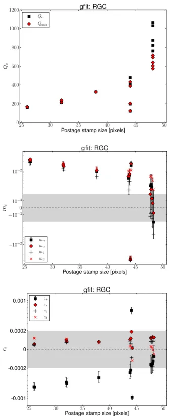
Given the importance ofσs, Fig.6shows the variation of our

metrics with this parameter. As shown in the top panel,Qcsharply

decreases for very smallσs, and reaches a maximum forσs≈1.

For infiniteσs(constant weighting), there are two submissions with

Figure 6. From top to bottom, we showQc,mi, and ci for the

Amal-gam@IAP team submissions as a function of theσsused in the weighting scheme, for all submissions in RGC. The target regions are shown as a grey shaded region, within which the vertical axis has a linear scaling; outside of the shaded region, the scaling is logarithmic. Note that the entries shown atσs=10 actually hadσs= ∞, i.e. completely equal weighting for all galaxies. Multiple submissions with the sameσshave slight horizontal off-sets for clarity. Themiandcipanels only show errors on a single quantity,

for clarity.

at California Institute of Technology on July 9, 2015

http://mnras.oxfordjournals.org/

quite differentQc values, 849 and 78, which we discuss in more

detail below.

The decrease inQc for very lowσsis quite interesting. Asσs

approaches zero, the weighting scheme gives a strong preference to very high-S/N galaxies. In real data, there is no advantage to giving such a preference because of shape noise. However, in GREAT3, we have cancelled out the shape noise by including 90◦rotated pairs, so in principle, a perfect shear estimate for just the two highest S/N galaxies would perfectly determine the shear for the whole field. The lowQcin this case implies that either the covariance matrix used

for the weighting is poorly determined or has some correlation with shear direction,orthat the shear estimates for high-S/N galaxies are poor. The high-S/N galaxies should have little noise bias, but may have model bias due to a mismatch between the input parametric models and the ones fitted by the Amalgam@IAP team. Another possible explanation relates to the adaptive selection of modelling window size (up to but not beyond the size of the input postage stamps). If the algorithm chooses too-small postage stamps for the highest S/N galaxies, it could introduce truncation biases as seen in GFITresults (see Section 4.1). Since a similar trend inQcwas

seen in CGC, the problem is not plausibly due solely to realistic galaxy morphology. Unfortunately given the data that we have, we are unable to tease apart these effects.

The other panels in Fig.6show themiandcivalues as a function

ofσs, to explain the trends in theQc plot. For very lowσs

(up-weighting the high-S/N galaxies), the multiplicative biases can be as bad as−7.6±0.5 per cent, with a very high detection signifi-cance for the trends inmi. For constant weighting, the submission

with near-zeromiandciincludes a penalty term on the aspect ratio,

whereas the poorly performing submission does not (giving a 10σ change inmi). In the bottom panel, asσsgoes from 0.05 up to 1 and

finally to∞(corresponding to strong S/N upweighting, weighting with a substantial shape noise term, and constant weighting, respec-tively),c₊goes from (3.2±0.2)×10−3_{, to consistent with zero,}

to negative values, (−4± 1)×10−4_{. The statistical significance}

of these changes is>10σ. This suggests thatc₊for this method is positive (negative) for the high- (low-) S/N galaxies.

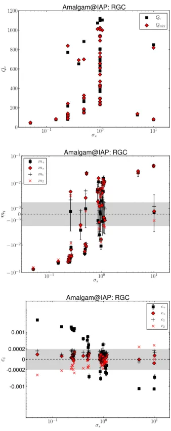
We now address the issue of the penalty term on aspect ratio, another parameter of interest that causes highly significant changes in multiplicative and additive biases as discussed above. The idea of the penalty term is that for galaxies that have low S/N and poor resolution, the ellipticity is so poorly determined that there is a very large tail to high ellipticity (which is a manifestation of noise bias). Hence, the idea is to penalize high ellipticity values by adding a term to theχ2_{, which will have little effect on}

high-ellipticity objects with high S/N. This was important particularly for fields with poor seeing and/or substantial defocus that enlarged

the PSF. An example is shown in Fig.7. The top panel shows the

fitted ellipticity distribution in a good-seeing (blue) and poor-seeing (red) field in GREAT3 without the penalty term, and the bottom panel shows the same when using the penalty term on aspect ratio. The distribution for the poor-seeing image has a pronounced high-ellipticity tail that is nearly removed by the penalty term, yet the shape of the distribution in the good-seeing image is less altered by the addition of this term.

In some sense, the addition to the term in theχ2_{is equivalent to}

multiplying the likelihood, i.e. imposing a prior on the ellipticity. It seems that this is a way to remove or reduce noise bias in all fields (with stronger impact on those that have poor seeing), eliminating the need for explicit calibration factors. For GREAT3, the best value of shape noiseσsto use in the weighting scheme and the form of the

penalty term to use in theχ2_{was clearly shown to do an excellent}

Figure 7. Fitted ellipticity distributions for the Amalgam@IAP team for a good-seeing (blue) and poor-seeing (red) subfield in GREAT3, in the CGC branch. The top (bottom) panel shows the results without (with) a penalty term on aspect ratio.

job at shear estimation for the particularp(ε) and galaxy property distributions used here. However, it is unclear whether these results would necessarily be consistently reproducible for other data sets with different intrinsicp(ε), or those with a p(ε) that correlates with other galaxy properties in a way that is not reproduced here. For this reason, further simulations would be needed to evaluate the generality of this procedure for real data with a variety of properties, and confirm that the exactσsand form of the penalty term gives

similar results in cancelling out noise bias.

4.2.2 Fair cross-branch comparison

For the Amalgam@IAP team, it was difficult to identify a single group of settings used for all branches. Instead, four groups of settings with submissions in a few branches were identified.

(1)χ2_{penalty term on aspect ratioθ}

aspect;σs=0.5 for weighting.

(2)χ2_{penalty term onθ}

aspect; uniform weighting (σs= ∞).

(3)χ2_{penalty term onθ}

aspectand S´ersic indexns;σs=0.5.

(4) No priors on model parameters;σs=0.5.

The settings also differed in minor ways that have little impact on performance.

Fig.8shows histograms ofQc,m, andc+values for all

Amal-gam@IAP submissions in all constant shear branches, also indicat-ing those submissions with the aforementioned consistent settindicat-ings with points. As shown, for branches that include submissions with setting 1, that submission is typically among the best in the branch, with RSC being the exception to this rule. This is consistent with our previous results indicating thatσs∼0.5 and theχ2penalty term

on aspect ratio were important factors affecting the results. Comparing the results for setting 1 and 2 in RGC, the only con-stant shear branch to include submissions with both settings, their performance seems quite consistent with each other. However, in variable shear branches (not shown), setting 1 leads to better per-formance, confirming the importance of the weight including both shape and measurement noise rather than using equal weighting.

at California Institute of Technology on July 9, 2015

http://mnras.oxfordjournals.org/

Figure 8. Top: histogram ofQcvalues for all submissions from the Amal-gam@IAP team for constant shear branches. The coloured points indicate submissions that are part of the fair cross-branch comparisons with con-sistent settings, with the four settings described in the text indicated with different shaped points. Middle, bottom: the same, but formandc+. The points have horizontal error bars indicating their statistical uncertainty, and the shaded regions indicate the target values ofmandc+. Outliers have been removed from the bottom two panels so that the main part of the distribution can be clearly seen.

Comparing settings 1 and 3, we see that for CGC, setting 1 leads to better performance due to a substantially smaller calibration bias. This suggests that use of a S´ersicnpenalty term is unimportant or perhaps even harmful, though its impact is somewhat less on vari-able shear branches (not shown). This finding may simply reflect the fact that the variable shear metric is less sensitive to multiplicative biasm.

Finally, settings 1 and 4 gave similar results, with comparablemi

andci. While the use of penalty terms onθaspectis helpful, that is

especially true for higherσsthan the value used here.

In general, the results for these fairly chosen sets of submissions are worse in CGC than in RGC. The primary reason is an average multiplicative bias ofm =0.8±0.2 per cent in CGC, whilem is consistent with zero in RGC. Since the simulation designs in the control and realistic galaxy experiments correspond apart from galaxy morphology, this difference between CGC and RGC sug-gests a model bias due to realistic galaxy morphology that is of that order. This bias may be cancelled out by some other bias in RGC (perhaps noise bias, truncation bias, or residual model bias due to mismatch between input and output parametric models). In contrast, the additive systematics for CGC versus RGC (setting 1) are consis-tent within the errors. For space branches, the multiplicative biases differ for RSC and CSC bymRSC− mCSC=0.80±0.15 per cent,

suggesting that model bias due to realistic galaxy morphology has a similar magnitude for both space and ground data.

4.2.3 Summary

Here, we summarize the key lessons from analysis of the Amal-gam@IAP results. First, the main factors that determine perfor-mance are the magnitude of shape noise used in the weighting scheme (σs) and the use of a penalty term on the aspect ratio to

reduce the incidence of spurious highly elliptical, lower S/N and resolution objects. Using the best choices for these parameters in all branches resulted in overall good performance, though with hints of a model bias for ground and space data due to realistic galaxy mor-phology that is slightly below a per cent. Also, strong variation in c₊with the weighting scheme suggests that the additive systematics are a strong function of the galaxy S/N.

Because of the importance ofσsand penalty terms in determining

performance, for the overall analysis and comparison with other methods, we use a set of submissions with the same value ofσs=0.5

and a penalty term on the aspect ratio, with small variations in other less important parameters.16

4.3 MegaLUT

4.3.1 Controlled tests of variation of parameters

The MegaLUT team (see Appendix C17) made many submissions with varying choices related to the learning sample generation, shape measurement, input parameters for the artificial neural net-work (ANN), architecture of the ANN, and finally the rejection of faint or unresolved galaxies. Here, we will explore the dependence of their results on these choices.

16_{For three variable-shear branches, there were no submissions with}

σs =0.5. To enable comparison in those branches, the Amalgam@IAP team made submissions after the end of the challenge using thesame cata-logues as during the challenge, reweighted usingσs=0.5.

at California Institute of Technology on July 9, 2015

http://mnras.oxfordjournals.org/

Figure 9. Top:mi values for four MegaLUT submissions in CGC with

different choices for how catalogues were filtered, but otherwise the same settings. Bottom:civalues.

First, we consider the filtering of the catalogues, comparing four submissions to CGC that used the same settings for all parameters except the filtering. Themiandcivalues for these four submissions

are shown in Fig.9, with theQcvalues indicated in the legend. As

shown, the results for the top three options (all with default filtering for positive flux and profile increasing) give very similar results, regardless of other choices like rejection based on maximum shear values, or clipping large shears (setting them to a maximum value of 0.9). However, removing the default filtering andonlyrejecting based on|g1|or|g2|>1 gives significantly worseQc. This is due

to bothmiandc+increasing in magnitude. This submission is only

mildly correlated with the others, and themiand cichanges are

only marginally significant (2σ). On a minor note, there is a 2σ–3σ hint of non-zeroc1andc2, which (if real) may reflect asymmetry

in selection criteria. Note that the default filtering option removes typically<1 per cent of the galaxies.

The next test was on CSC, comparing two otherwise similar submissions with different choices at the training stage. The training sample shears were uniformly distributed with |g|< 1 and with |g|<0.7. TheQcvalues were 289 and 228, respectively, primarily

because of a larger magnitude of the (negative) calibration bias in the latter case. This change inmis not very statistically significant (<2σ), which is interesting because it suggests a lack of sensitivity to this aspect of the training.

Also in CSC, we compare two submission that used different statistics of the image to describe the shape. In one submission, the adaptive moments routines inGALSIMwere used, effectively fitting

the image to an elliptical Gaussian; the other submission used the moments of the autocorrelation function (ACF; van Waerbeke et al. 1997) of the image. The results are shown in Fig.10.

Figure 10. Top:mivalues for two MegaLUT submissions in CSC with

dif-ferent methods of measuring galaxy shapes, but otherwise the same settings. Bottom:civalues.

TheQcvalues are 289 and 129, respectively, due to a 3σ

differ-ence inmivalues (the significance is larger than it appears on the

plot due to correlations between the submissions). Use of the ACF gives a more negative calibration bias ofm = −2.5±0.5 per cent, compared tom = −1.1±0.5 per cent without its use. Apparently the ACF is not an unbiased way of compressing the information in the image, consistent with what was seen for two methods using the

ACF in GREAT10 (Kitching et al.2012).

A final study performed in CSC relates to other ways of filtering the catalogues after shear estimates have been made, comparing the results of the default filtering with two other options; excluding

small objects, and using convex hull peeling (Eddy 1982). The

exclusion of small objects changesmiandcionly slightly. However,

convex hull peeling gives substantially worse results that are also

noisier, withQc reduced from around 300 to 113, andmgoing

from−1.1±0.5 to 3±1 per cent (4σ significance).

For RSC, we compared two submissions with different train-ing options. In one case (‘half noise’), the traintrain-ing set images had noise that was half the level in the GREAT3 images; in the other case, it was ‘low noise’, 1/10 the level in the GREAT3 im-ages. Fig.11shows that the latter gives significantly better perfor-mance,Qc=221 instead of 139. The ‘half noise’ case has slightly

worsemivalues, and substantially worse additive systematics of

c+ = (10 ± 1) ×10−4 _{versus c}

+ = (−3± 2) ×10−4 _{in the}

low-noise case, a 5σdifference given the correlations between the submissions). The increase inmiwith increasing noise in the

train-ing sample images could be due to the resulttrain-ing noisiness in the input features of the ANN training. This noisiness smears out any sharp structures that the ANN regression should fit, leading to

bi-ased ANN predictions. We speculate that the effects onc₊ may

at California Institute of Technology on July 9, 2015

http://mnras.oxfordjournals.org/