Analysis of Land Use Spatial Patterns in Coastal Andhra Region Using Remote Sensing, GIS and Computational Techniques

Technology (IJRASET)

Analysis of Land Use Spatial Patterns in Coastal

Andhra Region Using Remote Sensing, GIS and

Computational Techniques

Md. Ateeque A Khan1, Jai Kumar2, A. P. Krishna3 1,2,3

Department of Remote Sensing, Birla Institute of Technology, Ranchi, Jharkhand, India

Abstract: It is well known fact that urbanization is a prime aim of all the developing cities of India, Since 2010, infrastructure development has been the utmost priority of Indian government. This urbanization of cities, villages has led to need of planned decisions and allocation of domestic units at alarming rates. The purpose of this study is to access to spatio-temporal variation of LU/LC in Andhra Pradesh region using Landsat 4,5 TM & Landsat 8 OLI imagery during the study period of 1991 to 2006 & 2006 to 2014. Through this period it has been found that there has been gradual increase in landscape classes i.e., built up, agriculture, forest but decrease in wasteland and water & this change was used as input variable for the markov model for the prediction of the year 2030, to get an idea of the probable change that could occur in the LU/LC classes for understanding the behavior change of respective classes. This prediction model was tested with the actual values with predicted values of the classified image classes changes for the year 2006 to 2014, & then checked by goodness of fit test (Chi-square test) for the validation of the predicted data. This change of landuse land cover study can be used for the planned development of the cities while keeping in consideration already developed units and this database can prove to be a useful for the better understanding and prediction of the factors depending over this features like the population growth, agriculture production, etc. Keywords— Spatio-Temporal Variation, LU/LC, Markov Model, prediction, ChiSquare Test

I. INTRODUCTION

A series of human operations on land with the interaction to obtain products & benefits using land resources, which covers earth surface, water resources, bare rocks, wet lands etc., causes the change in the natural development of the region and affects the natures weathering process occurring in the respective region observing land use/land cover change through the years in features which are identified through Remote sensing techniques like built-up, forest, agriculture etc., Area-wide land use and land cover mapping projects (Civco and Hurd, 1999) have utilized multi-temporal and multi-resolution remote sensing data (Zhou and Civco, 1998). Recent efforts have addressed improved methods for LULC change detection (Hurd et al., 2001), and hierarchical image segmentation and object-oriented LULC classification. This database was then used to analyze and interpret the changes occurring in the area of study so as to monitor these changes for the balanced development between nature – human sustenance. In this study, using landuse maps (1991, 2006, and 2014 years), and natural and socioeconomic data, we combine Markov model with GIS technology to successfully simulate the land use changes in region of study. Facing to declining problems of urban land in the area context. The simulated future land use maps can serve as an early warning system for understanding the future effects of land use changes. The acquired information is beneficial to other communal areas in Andhra Pradesh, experiencing similar land use changes. The simulation results can also be considered as a strategic guide to urban land use planning, and help local authorities better understand a complex land use system and develop the improved land use management that can better balance urban expansion and ecological environment conservation.

II. STUDY AREA

Technology (IJRASET)

recent decades. The population growth in my region has founded to be at rate of 10% - 12 % from the period of 1991 – 2001 & 2001 – 2011, according to the Census data of Andhra Pradesh, resulting in of high to average population density of 441 persons per square kilometer.

Figure 1: Study Area

A. Objectives of Study

To quantify the spatial patterning of land cover patches, land cover classes, or entire landscape mosaics of a geographic area & to identify the developmental/degradation effects of the changes over the study area in favour of the balanced development and intelligent use of resources available for the social & economic development of the area.

B. Techniques

1) LULC Classification

2) Change Detection Identification between years 1991 - 2014

3) Change Prediction using Markov Model

C. Data Used

Landsat 4- Thematic Mapper year of Acquisition(may-june1991) ,Lansat5- Thematic Mapper year of Acquisition(may-june 2006) Landsat 8 Operational Land Imager year of Acquisition (may-june 2014)

Technology (IJRASET)

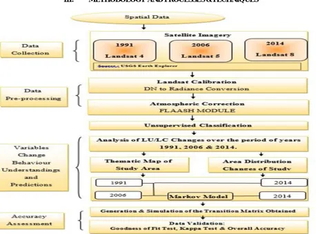
III. METHODOLOGY AND PROCESSES &TECHNIQUES

Figure 2: Methodology

C. Processes & Techniques

1) Atmospheric Corrections: Atmospheric correction is a major issue in visible or near-infrared remote sensing because the presence of the atmosphere always influences the radiation from the ground to the sensor. Dust, haze effect, Rayleigh scattering are the common phenomena’s which are responsible for the false capture of the satellite sensor over the region.

(a)FLAASH (Fast Line-of-sight Atmospheric Analysis of Hyper cubes):

It is the type of corrections which helps out in removal of aerosol & dust particle haze effect over the region of tropical and sub-tropical regions of planet for the landsat images. Usually many other atmospheric correction programs that interpolate radiation transfer properties from a pre-calculated database of modeling results, FLAASH incorporates the MODTRAN radiation transfer code. You can choose any of the standard MODTRAN model atmospheres and aerosol types to represent the scene; a unique MODTRAN solution is computed for each image.

2) FLAASH also includes the following features: Correction for the adjacency effect (pixel mixing due to scattering of surface-reflected radiance)

An option to compute a scene-average visibility (aerosol/haze amount). FLAASH uses the most advanced techniques for handling particularly stressing atmospheric conditions, such as the presence of clouds.

Cirrus and opaque cloud classification map

Adjustable spectral polishing for artifact suppression.

Technology (IJRASET)

Where:

ρ is the pixel surface reflectance

ρe is an average surface reflectance for the pixel and a surrounding region S is the spherical albedo of the atmosphere

La is the radiance back scattered by the atmosphere

A and B are coefficients that depend on atmospheric and geometric conditions but not on the surface.

Each of these variables depends on the spectral channel; the wavelength index has been omitted for simplicity. The first term in Equation (1) corresponds to radiance that is reflected from the surface and travels directly into the sensor, while the second term

corresponds to radiance from the surface that is scattered by the atmosphere into the sensor. The distinction between ρ and ρe accounts for the adjacency effect (spatial mixing of radiance among nearby pixels) caused by atmospheric scattering. To ignore

the adjacency effect correction, set ρe = ρ. However, this correction can result in significant reflectance errors at short wavelengths,

especially under hazy conditions and when strong contrasts occur among the materials in the scene.

The values of A, B, S and La are determined from MODTRAN calculations that use the viewing and solar angles and the mean surface elevation of the measurement, and they assume a certain model atmosphere, aerosol type, and visible range.

The values of A, B, S and La are strongly dependent on the water vapour column amount, which is generally not well known and may vary across the scene. To account for unknown and variable column water vapour, the MODTRAN calculations are looped over a series of different column amounts, then selected wavelength channels of the image are analysed to retrieve an estimated amount for each pixel. Specifically, radiance averages are gathered for two sets of channels: an absorption set centered at a water band (typically 1130 nm) and a reference set of channels taken from just outside the band. A lookup table for retrieving the water vapour from these radiances is constructed.

After the water retrieval is performed, Equation (1) is solved for the pixel surface reflectances in all of the sensor channels. The solution method involves computing a spatially averaged radiance image Le, from which the spatially averaged reflectance ρe is estimated using the approximate equation:

Spatial averaging is performed using a point-spread function that describes the relative contributions to the pixel radiance from points on the ground at different distances from the direct line of sight. For accurate results, cloud-containing pixels must be removed prior to averaging. The cloudy pixels are found using a combination of brightness, band ratio, and water vapour tests, as described byMatthew et al. (2000).

The FLAASH model includes a method for retrieving an estimated aerosol/haze amount from selected dark land pixels in the scene. The method is based on observations byKaufman et al. (1997)of a nearly fixed ratio between the reflectance’s for such pixels at 660 nm and 2100 nm. FLAASH retrieves the aerosol amount by iterating Equations (1) and (2) over a series of visible ranges, for example, 17 km to 200 km. For each visible range, it retrieves the scene-average 660 nm and 2100 nm reflectance for the dark pixels, and it interpolates the best estimate of the visible range by matching the ratio to the average ratio of ~0.45 that was observed byKaufman et al. (1997). Using this visible range estimate, FLAASH performs a second and final MODTRAN calculation loop over water.

3) Spectral Polishing: Spectral polishing is a term used byBoardman (1998)for a linear re-normalization method that reduces spectral artifacts in hyperspectral data using only the data itself. The basic assumptions are as follows:

The FLAASH polishing algorithm yields similar results with less input data. The smoothing is performed with a running average overnadjacent channels (wherenis defined as the polishing width). Spectrum endpoint and missing-channel complications are limited if only a modest amount of smoothing is desired (nis low).

Technology (IJRASET)

4) Wavelength Calibration: An accurate wavelength calibration is critical for atmospherically correcting hyperspectral data. Even slight errors in the locations of the band centre wavelengths can introduce significant errors into the water retrieval process, and reduce the overall accuracy of the modeled surface reflectance results.

You find that the corrected wavelengths are an improvement after the FLAASH processing is complete, upon applying them to the original input radiance image.

D. Change Detection

Land use and land cover (LULC) change and degradation Land degradation patterns have been associated with land‐use and land‐

cover changes. Land cover refers to the physical characteristics of the earth surface, captured in the distribution of vegetation, water, desert, ice and other physical feature of the land including those created solely by human activities such as mine exposures and settlement (FAO 1997). On the other hand, land use is a term used to describe human uses of the land, or immediate actions modifying or converting land cover (FAO 1997; de Sherbinin 2002).

Land‐cover and land‐use change can be classified into two broad categories: conversion or modification (Butt and Olson 2002). Conversion refers to the changes from one cover or use to another, e.g. conversion of forests to pasture or to cropland. Modification on the other hand refers to the maintenance of the broad cover or use type in the face of changes in its attributes. For example, a forest may be retained but significant alterations may be made on its structure or function. The key LULC change pathways include deforestation, desertification, wetland drainage and agricultural intensification (Butt and Olson 2002). The pathways can be envisioned as forcing functions, which have direction (forest to pasture or pasture to cropland), magnitude (amount of change), and pace (rates of change).

LULC changes reflect the complex interaction of human activities and environmental processes over time and space on land. Humans play a key role in contributing to the process and are equally affected by these LULC changes. Whereas the major reasons for such LULC changes are positive and aim to increase the local capacity to support the human enterprise, there are also unforeseen negative impacts that can reduce the ability of land to sustain the human enterprise (Houghton 1994). Understanding LULC changes is therefore critical for the design of effective land management programs.

Table 1: Change Detection Procedure (Source: Lackey et al. 1994)

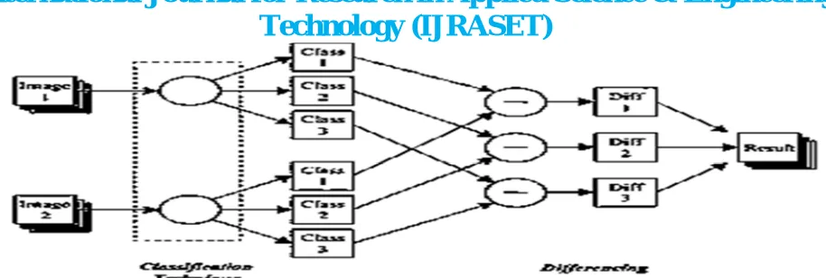
1) Post-Classification Techniques: This approach is based on rectification of more than one classified image; where it involves the classification of each of the images independently, then the thematic maps are generated, followed by a comparison of the corresponding labels or themes to identify areas where change has occurred. There are several advantages to this technique: it minimizes sensor, atmospheric, and environmental differences because data from two dates are separately classified, thereby minimizing the problem of normalizing for atmospheric and sensor differences between two dates and it provides a complete matrix of land cover change when using multiple images (Lu et al. 2004, Jensen 2005, Naumann, Siegmund 2004, Teng et al. 2008). A series of “from-to” matrixes can be built by comparing on a pixel by pixel basis, and these matrices include pixel conversion matrix, percentages conversion matrix, and area conversion matrix. However, results derived from this method are only as accurate as the individual classification images themselves.

C

h

an

ge

D

et

ec

ti

on

P

roc

ed

u

re

1. Nature of change detection problems

2. Selection of Remotely sensed data

3. Image preprocessing

4. Image processing / Classification

5. Selection of Change Detection Algorithms

Technology (IJRASET)

Figure 3: Diagram of Post-classification Comparison Change Detection (Source: Lackey et al,. 1994)

E. Assessment of LULC change

LULC can be assessed at different scales (hierarchy theory): field to farm, the community, the landscape, and national/continental and global levels (LADA 2009).The different scales of analysis provide different types of information. Global and continental LULC assessment outputs are general in nature and hence are suitable for long‐term global environmental change studies such as global climate change and biogeochemical cycles. Conversely, studies at landscape and farm levels are more detailed and provide insights on the actual causes and changes taking place at a given location; such information can aid in designing strategies for rehabilitation and Background restoration. Studies undertaken at national levels are often used for policy formulation and resource allocation. The benefit of the hierarchical approach is that the findings from one scale can be used to verify the interpretation of information from other scales. It is how ever worth noting that data at different scales may seem to be contradictory although allare correct. Processes at different scales may be completely different, hence it may not be possible to directly ‘scale‐up’ the results from a local analysis to higher levels by simple aggregation, nor to ‘down‐scale’ by ascribing group attributes to individuals (Olson et al. 2004). This is because the different scales are associated with hierarchies of social order, with each level having different actors, (e.g., national government, local government, household, individual) with separate functions, activities and environmental management effects (Blaikie and Brookfield 1987). Similarly, it is important to evaluate how policies vary with scale of assessment (Turner II et al.1995). Adopting a multi‐scalar approach is therefore needed to strengthen both the interpretation and use of LULC data for designing effective sustainable landmanagement programs.

LULC analysis usually involves the interpretation of geographical or spatial information from aerial photographs, satellite images, ground measurements or maps.By interpreting data from different time periods, temporal changes in the landscape can be determined (Pinheiro et al. 2007). Linking the land use and other spatial data such as roads, elevation or administrative boundaries in a geographical information systems (GIS), allows enhanced interpretation of the land‐use information. Over the years, interest in LULC change studies has grown due to improved availability of remotely sensed data and facilitated analysis software. For example, the United States Geological Survey (USGS) has provided access to a wide range of satellite imagery, some free of charge, which can be used for LULC change assessments. Apart from the commercial remote sensing and GIS software applications (e.g., ArcGIS,IDRISI, ENVI, ERDAS), many open source software (e.g., ILWIS, QGIS, GRASS) withsimilar capabilities have been developed and made available to researchers and landmanagers. As a result, LULC has been mainstreamed into global environmental change background research because it provides broad‐scale data on aspects such as climate change,changing carbon stocks, habitats and biodiversity. It provides an entry into understanding the human dimensions of environmental change (Turner II et al. 1995;Lambin et al. 1999; de Sherbinin 2002).By examining information across time periods or between variables, processes can be identified. Such processes may include changing size, distribution and diversity of landscapes/habitats, relationships between land tenure and landmanagement practices, differential impact of policy on land development or use, andemerging pressures/competition on a given resource among others. With this information on spatial patterns and processes, answers to questions on where changeis taking place and why it is taking place can be provided. It is more effective andsustainable to address the underlying root causes of degradation or loss than to try to address the consequences.

Technology (IJRASET)

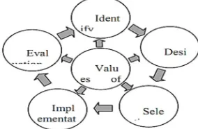
predictor variables. Remotely sensed variables, like the normalized difference vegetation index (NDVI), which is a measure of photosynthetic ‘‘greenness’’ (Tucker and Sellers 1986), have been used to inform models predicting the occurrence of plant and animal species (Gould 2000, Muldavin et al. 2001, Kerr and Ostrovsky 2003, Gillespie 2005). Among the requirements for application of remotely sensed data to predict and manage the spatial dynamics of landuse changes is the ability to accurately identify distribution patterns of required factors through time. Importance of User's Participation in Process Design Armstrong (1993) observed that the individual has a natural claim to participate in decision making related to his/her situation with both psychological and social needs to feel control over his or her own life conditions. He explains that decisions become better when the persons who are affected become a part of the decision making process. If one longs for decision making and esteems the design of expert and participative technical solutions over those designed through , object and realization design, the technical/ participative approach is likely to be used. Main stages of the design process can comes into account a general decision model: Identify, design, selection, implementation and evaluation of environment are the main stages of the design process

Figure 4: Decision Analysis Function Cycle

F. Markov Chain

On a spatial grid, a Markov chain is a random process where the state of a pixel depends only its immediate neighbors. The probability that a pixel has a certain value can be computed based on the values of its neighbors. The Markov model is a theory based on the process of the formation of Markov random process systems for the prediction and optimal control theory method. The Markov model not only explains the quantification of conversion states between the land use types, but can also reveal the transfer rate among different land use types. It is commonly used in the prediction of geographical characteristics with no aftereffect event which has now become an important predicting method in geographic research. Based on the conditional probability formula— Bayes, the prediction of land use changes is calculated by the following equation

S(t + 1) = Pij × S(t)

where S(t), S(t +1) are the system status at the time of t or t +1; Pij is the transition probability matrix in a state which is calculated as

follows

Technology (IJRASET)

lengthencoding where runs of the same value are compressed so that only changes in the pixel value within the grid need to be stored.

Markov model has been used to represent change in land use and land cover at different spatial and temporal levels. Land use studies using markov chain models have a proclivity to focus on a large spatial level and engage both built up and non-built-up cover land (Bell, 1974: Muller and Middleton, 1994: Weng, 2002). Markov model have so many assumption (Bell, 1974: Weng, 2002). One important is that it considers LULC as a stochastic process and different categories of land use are as the states of chain. A chain is defined as Stochastic process having the conditional probability distribution of the process at time n+1, Xn+1depends upon

only value of Xn and its not dependent on all other previous value Xn-1, Xn-2…….X0

As mentioned earlier,

P[Xn+1 = xn+1 | Xn] = xn,…….X0 = x0P[Xn+1 = xn+1|Xn = xn] – 1

This can also expressed as

Pij = P[Xn+1 = j| Xn = i] - 2

ij = 0,1,2,……….

Here Pij is transition probability of one step, can be analyzed as the conditional probability at time n when the process in state I and

at time n+1 the process is in state j.

Two step transition probability is defined with generalization of Chapman-Kolmogorov equalization. Pij(2) = P[Xn+2 = j | Xn = i] = ∑P[Xn+2 = j|Xn+1 = k]P[Xn=k|Xn=i] – 3

This is equivalent to

Pm+n = Pn/Pm

Hypothesis test for statistical independence:

To follow the hypothesis of statistical independence involves a process of comparing the actual data with expected data of land use using following formula

K2 = ∑i∑j(Aik – Eik)2/Ea

Where,

Eik = Expected value under markov hypothesis

Aik = Actual value of the data from category in I to category in k

If the value of K2 is greater than the tabulated value on the critical region 0.05 with the degree of freedom (D.F.-1)2 the hypothesis will be rejected. The expected value calculated with the help of Chapman-Kolmogorov equation following the markov method. For the calculation of transition probability matrix for the period 1991-2014 can be obtained by multiplying the 1991-2006 & 2006-2014 classified images. This expected value is calculated by following formula

Eik = (Eij)(Ejk)/Ej

Where,

Eij = the number of transition from category I to j during the period 1991 – 2006.

Ejk = the number of transition from category I to j during the period 2006 - 2014.

Ej = the number of cells in the category j in 1991.

3.5.5 Statistical Tests

G. Kappa Statistics

Technology (IJRASET)

Where

Pr(a) is the relative observed agreement among raters, and Pr(e) is the hypothetical probability of chance agreement,

using the observed data to calculate the probabilities of each observer randomly saying each category.

If the raters are in complete agreement then κ = 1. If there is no agreement among the raters other than what would be expected by chance (as defined by Pr(e)), κ = 0

H. Test of Goodness of Fit

Chi square test of goodness of fit is used to test first order Markovian suitability with the data. This test analyses that particular distribution adequately described or not. By making comparison between actual observed probability and expected probability.

Xc2 = ∑i∑j(Oik – Eik)2/Eik

Where

Oij = Observed transition probability data from 1991 - 2014

Eij = the number of transition from category I to j during the period 1991 – 2014

If the Xc2 is less than the value of X1-a on the 0,05 critical region then the hypothesis is accepted.

Markov model for land use and land cover have not been in essence with the use of satellite data and remote sensing technology. The most of the study based on Markov model for land use changes based on field surveys or existing maps and data (Bell, 1974; Muller and Middleton, 1994). So uncertainties in data are very high in this situation but with the use of remote sensing data this uncertainty can be removed and quality of input data for analysis can be improved. Markov chain is very rarely used to model dynamics of land use and land cover in developing countries.

IV. EXPERIMENTAL RESULTS

Technology (IJRASET)

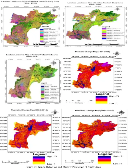
end up with the graphical representation of the quantified areal changes observed after the LU/LC classification , along with it the prediction for the year of 2030 using Markov technique has resulted in giving us an understanding for the change re-presentation observed from the year 1991 – 2014, and 2014 – 2030

Technology (IJRASET)

The transition probabilities has been calculated for the years 1991 - 2006, 2006 - 2014 & 1991 - 2014. In table 2 & 4 the observed transition of the years 2006 - 2014 & 1991 - 2006 has been shown, along with the formulated transition calculated by the markov chain model was compare, to check the Markovian suitability with the help of hypothesis of goodness of fit test. In this test the actual change observed calculated by manual simulations and change observed by markov chain model was tested and the chi-square value was obtained as 2.76 & 8.68 which is less than 14.78, the significance limit on critical region 0.05 with the degree of freedom of (8-1) = 7. With acceptance of the hypothesis one can say that actual transition probability of matrix from 1991 - 2014 is fitted with expected transition probability prepared using markov method.

Table 2: Observation Transition 2006 - 2014

0 1 2 3 5 6 7 8

0 0.9296 0.003281812 0.024669236 0.007701 0.011135 0.004843 0.018589 0.000181 1 0.01261 0.10943287 0.493158411 0.199203 0.09876 0.061366 0.017361 0.008109

2 0.002173 0.077445576 0.430376792 0.135288 0.218938 0.116008 0.016773 0.002997

3 0.00368 0.033271655 0.287694844 0.438791 0.192322 0.034213 0.008181 0.001847 5 0.002185 0.058624692 0.291412649 0.076514 0.406258 0.154816 0.009673 0.000516

6 0.002558 0.042253901 0.248859291 0.058427 0.241396 0.36747 0.036638 0.002398

7 0.023969 0.005205123 0.065820843 0.006753 0.012944 0.013022 0.868496 0.003791

8 0.0072 0.022142708 0.298576451 0.201474 0.267987 0.172043 0.030077 0.000499

Deduced Transition using Markov Chain Model

Table 3: Formulated Transition 2006 - 2014

Cl. 1 Cl. 2 Cl. 3 Cl. 5 Cl. 6 Cl. 7 Cl. 8 Cl. 15

Class 1 0.1358 0.7347 0.1033 0.01 0.015 0.0048 0.0064 0.07456

Class 2 0.0917 0.4587 0.1202 0.2022 0.1061 0.0175 0.0037 0.0732 Class 3 0.0043 0.1871 0.6919 0.1153 0.01 0.0004 0.0011 0.0456

Class 5 0.0451 0.2829 0.015 0.5389 0.1181 0.01 0.01 0.0676 Class 6 0.0171 0.171 0.01 0.2037 0.5924 0.0146 0.0011 0.0866

Class 7 0.0374 0.1443 0.0223 0.0621 0.0519 0.6803 0.0018 0.0334 Class 8 0.01 0.2677 0.2402 0.2679 0.1957 0.0285 0.01 0.01

Class15 0.0014 0.0014 0.0014 0.0014 0.0014 0.0014 0.0014 0.98

Technology (IJRASET)

Table 4: Observed Transition 1991- 2006

0 1 2 3 5 6 7 8

0 0.010067 0.064468713 0.176736905 0.090747 0.071029 0.578756 0.005398 0.002798 1 0.033332 0.502911457 0.189002796 0.173441 0.054028 0.023855 0.017109 0.006323 2 0.039131 0.43642949 0.211505705 0.192406 0.055098 0.037017 0.025129 0.003284 3 0.018639 0.35917744 0.405662434 0.121 0.038677 0.021773 0.032899 0.002171 5 0.021178 0.35159546 0.173127799 0.303226 0.08833 0.024516 0.03767 0.000357 6 0.042232 0.323080634 0.085999095 0.240459 0.134244 0.092185 0.07863 0.003171 7 0.000833 0.012694654 0.007411809 0.007075 0.006334 0.959569 0.001787 0.004296 8 0.014508 0.119086349 0.293328133 0.267968 0.018588 0.284696 0.00056 0.001265

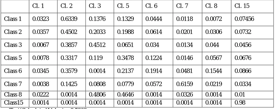
Table 5: Formulated Transition 1991 - 2006

Cl. 1 Cl. 2 Cl. 3 Cl. 5 Cl. 6 Cl. 7 Cl. 8 Cl. 15 Class 1 0.0323 0.6339 0.1376 0.1329 0.0444 0.0118 0.0072 0.07456 Class 2 0.0357 0.4502 0.2033 0.1988 0.0614 0.0201 0.0306 0.0732 Class 3 0.0067 0.3857 0.4512 0.0651 0.034 0.0134 0.044 0.0456 Class 5 0.0078 0.3317 0.119 0.3478 0.1224 0.0146 0.0567 0.0676 Class 6 0.0345 0.3579 0.0014 0.2137 0.1914 0.0481 0.1544 0.0866 Class 7 0.0038 0.1425 0.0808 0.0779 0.0572 0.6159 0.0219 0.0334 Class 8 0.0222 0.0014 0.4806 0.4646 0.0014 0.0326 0.0014 0.01 Class15 0.0014 0.0014 0.0014 0.0014 0.0014 0.0014 0.0014 0.98 Chi-Square Test(Calculated Value) = 8.5803

Using these transition probabilities and Markov chain, the area distribution of the respective classes were predicted through the help of Terrset software (IDRISI Pvt. Ltd)

Table 6: Area in Km2

Class Area in Km

2

1991 2006 2014 2030 Unclassified 2944.2159 3559.36 1622.2995 4568.555

Built-Up 4124.8512 4824.851 5509.6614 6234.789 Agriculture 37376.757 38821.42 39067.5744 42056

Forest 23589.9828 24478.71 25478.98 28656.44 Waste 33497.7705 22830.3 27427.518 19564.98 Wet 5775.1749 8526.291 9420.824 7024.359 Water 3504.4731 4375.082 3471.0822 3953.245 Clouds 1367.9415 4765.153 183.2382 123.556

Technology (IJRASET)

Table 7: Area Distribution in Percentage Area in Percentage

LU/LC CLASSES

1991 Area in %

2006 Area in %

2014 Area in %

2030 Area in %

Observed Change in %

Predicted Change in % Unclassified 2.62% 3.17% 1.45% 4.07% -81.4841 35.55433468

Built-Up 3.68% 4.30% 4.91% 5.56% 25.13422 33.84092242 Agriculture 33.32% 34.61% 34.83% 37.49% 4.32793 11.12562317

Forest 21.03% 21.82% 22.71% 25.54% 7.413944 17.67944251

Waste 29.86% 20.35% 24.45% 17.44% -22.132 -71.2140888 Wet 5.15% 7.60% 8.40% 6.26% 38.69777 17.78305081

Water 3.12% 3.90% 3.09% 3.52% -0.96197 11.35139293 Clouds 1.22% 4.25% 0.16% 0.11% -646.537 -1007.15034

Total Area 100.00% 100.00% 100.00% 100.00% - -

V. CONCLUSION

My study region lies on EasternGhats of Indian coast of India where there is a high density of lineaments & fracture zones with the igneous & metamorphic rocks with partially sedimentary lithology along the coast line of India. Rainfall & humidity is seasonal & comes in adequate amount for life existence.

The study area cover 9 districts located between 13.701° and 18.276°N latitude and 78.165° and 82.585°E longitude& major urban settlements in the region are Vijayawada, Vishakhapatnam, Kadapa, Guntur, Prakasham, Nalgonda, Khammam, Nellore & has 5 major river flowing through it. Land is becoming scarce commodity due to immense agriculture & demographic pressure. Due to the coastal geomorphology & coastal plains along with enriched vegetated zones, it has been observed fast expanding township in the study region & now it has become crucial to evaluate the present day LULC & its dynamics over a period of time.

The present status of LULC in study area region was mapped using satellite images of the year 1991 to 2014 & statistics on its dynamics over a period of about two and a half decade was evaluated by comparing the major categories undergone change with respect to topographical map of the study area prepared during the year 1991.

The various categories of the landuse land cover interpreted in coastal Andhra can classified into five major groups, built-up land (4%), agriculture land (38%), forest land (23%), shrubs wasteland (25%), & water bodies (4%). The landuse in the study region is dominated by fallow land & shrubs wasteland with small areas of forest & barren land. Parts of city, coastal areas & highways form parts of settlements.

The results of LULC dynamics clearly indicated the landuse pattern in the study area has changed substantially. The overall changes in the built-up land from 4124.54 Km2 in 1991 to 5509 Km2in 2014 indicating 25% increase in total Built-up area. The forest cover increased by 7.4% of the total forest cover during the period from 1991 to 2014.

Technology (IJRASET)

and this change has been observed in coastal region or in the parts of routes along the highways.

Remote Sensing has proved its potential in a assessing the LULC cover of 9 districts & monitoring major changes over period of about 30 years. The satellite mage based prospects evaluation has certainly provided insight into the potential of development over the period of time. GIS proved to be powerful tool in spatial computations and analysis for quantifying the change detection techniques and a major tool for the preparation of the transition matrix for the application of the Markov model for the prediction analysis of the study area.

Aft er th e database h as been pr epar ed for th e simulation s, we have tr ied to descr ibe h ow th e Mar kov m od el with combination of remote sensing is used to explore the change in land use and land cover of parts of Telengana & Andhra Pradesh during the period 1991 - 2014. The Markov model has enormous capabilities to show the trend and projection of the land use and land cover. The interpretation fr om this can be used as a magnitude and direction of change in land use and land change in the future. The study of land use and land cover change is enhanced by integration of remote sensing and with Markov model. The quality of input data for analysis has been improved using GIS and remote sensing data.

Finally we conclude that Markov model based analysis gives better

VI. ACKNOWLEDGMENT

I would like to extend my gratitude to my guide, Dr. A. P. Krishna, Head of Department of Remote Sensing, B.I.T. Mesra, Ranchi, for giving me the permission to carry out the project and for devoting his valuable time and always being a constant source of advice and inspiration without which this work wouldn’t have been possible.

REFERENCES

[1] Al-shalabi, et al,. (2013) “Modelling urban growth evolution and land-use changes using GIS based cellular automata and SLEUTH models: the case of Sana’a metropolitan city, Yemen.” Environmental Earth Science :1–13

[2] Al-sharif AAA, Pradhan B (2013) “Urban sprawl analysis of Tripoli Metropolitan city (Libya) using remote sensing data and multivariate logistic regression model”. J Indian Society of Remote Sensensing:1–15.

[3] Alexandrov GA, Oikawa T (1997) “Contemporary variations in terrestrial net primary productivity: the use of satellite data in the light of the external principle.” Ecological Modeling 95:113‐118

[4] Allen JC, Barnes DF (1985) “The causes of deforestation in developing countries.” Annals of the Association of American Geographers 75 (2):163–184 [5] Bastin GN, Pickup G, Pearce G (1995) “Utility of AVHRR data for land degradation assessment: a case study.” International Journal of Remote Sensing 16

(4):651‐667

[6] Bell, Earl J. (1974) "Markov analysis of land use change—an application of stochastic processes to remotely sensed data." Socio-Economic Planning Sciences : 8.6 311-316.

[7] Berk, A., et al. (1998) "MODTRAN cloud and multiple scattering upgrades with application to AVIRIS." Remote Sensing of Environment 65.3 : 367-375. [8] Chander, G.,Meyer, D. J., & Helder, D. L. (2004). “Cross-calibration of the Landsat-7 ETM+ and EO-1 ALI sensors.” IEEE Transactions on Geoscience and

Remote Sensing, 42(12), 2821−2831.

[9] Civco, Daniel L., et al. (2002) "A comparison of land use and land cover change detection methods." ASPRS-ACSM Annual Conference..

[10] Felde, G. W., et al. (2003) "Analysis of Hyperion data with the FLAASH atmospheric correction algorithm." Geoscience and Remote Sensing Symposium, IGARSS'03. Proceedings. 2003 IEEE International. Vol. 1. IEEE.

[11] Fuglsang, Morten, Bernd Münier, and Henning Sten Hansen. (2013) "Modelling land-use effects of future urbanization using cellular automata: An Eastern Danish case." Environmental Modelling & Software 50 : 1-11.

[12] Guan, DongJie, et al. (2011) "Modelling urban land use change by the integration of cellular automaton and Markov model." Ecological Modelling 222.20 : 3761-3772.

[13] Rao, K. Nageswara, et al. (2013) "Geomorphological implications of the basement structure in the Krishna-Godavari deltas, India." Zeitschrift für Geomorphologie 57.1 : 25-44.

[14] Stefanov, W. L., et al. (2007) "Applied remote sensing for urban planning, governance and sustainability." : 137-64.

[15] Sang, Lingling, et al. (2011) "Simulation of land use spatial pattern of towns and villages based on CA–Markov model." Mathematical and Computer Modelling 54.3 : 938-943.