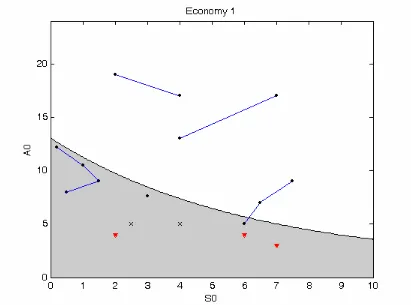
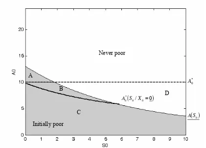
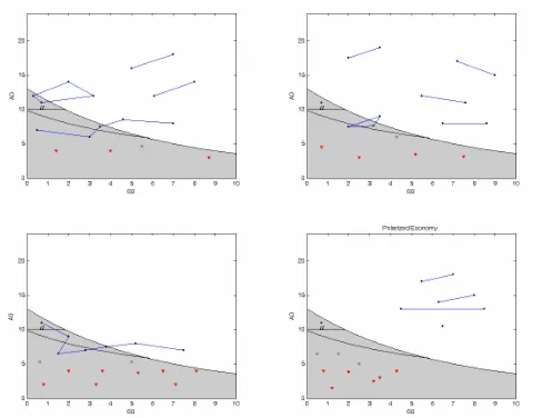
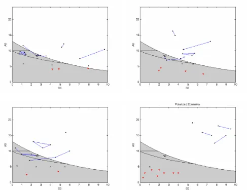
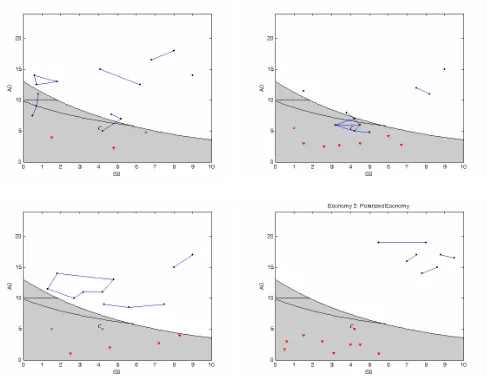
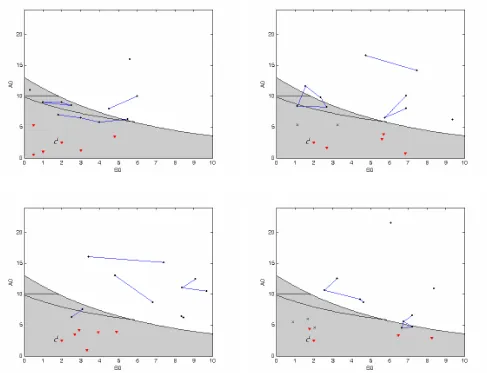
Social Network Capital, Economic Mobility and Poverty Traps

photoluminescence intensity by co-doping with alkali metal ions in CaO:Sm 3+ is due to the generation of oxygen vacancies to promote energy transfer from Ca 2+ to Sm 3+ and

Once the preprocessed features are extracted, machine learning methods can be used to develop the classification model for sentiment analysis.. After the crucial investigation

• After participating in mentoring activities, faculty is : (1) ready to perform RPP for large group student, (2) capable to make continuous improve- ment for teaching, and

Your Chance to Make it Better.  AmeriCorps is your chance to put your ideas into action while learning new skills, making new connections, and earning money to pay for education.

Archery Family Travel 1 Make a list of things to take on a 3-day trip Nutrition 1 Make a poster of foods that are good for you Video Games 1 Explain the rating system. BB Gun Shooting

It receives support from the World Bank, UNDP, the Kenya Gatsby Charitable Trust, the Global Fund for Women, Trickle-Up, the Government of Kenya, the Consultative Group to Assist

Data over five years old is freely accessible Database and associated with FOODSHIELD a collaborative platform and the Intentional Adulteration Assessment Tool (IAAT)

Therefore, the objective of this work is to propose a new procedure for analyzing and fitting response surface models to mixed experiments of two- level, three-level