http://dx.doi.org/10.4236/ojs.2016.64059
How to cite this paper: van Heel, M., Portugal, R.V. and Schatz, M. (2016) Multivariate Statistical Analysis of Large Datasets: Single Particle Electron Microscopy. Open Journal of Statistics, 6, 701-739. http://dx.doi.org/10.4236/ojs.2016.64059
Multivariate Statistical Analysis of Large
Datasets: Single Particle Electron
Microscopy
*
Marin van Heel
1,2,3, Rodrigo V. Portugal
3, Michael Schatz
41Institute of Biology Leiden, Leiden University, NeCEN, Leiden, The Netherlands 2Sir Ernst Chain Building, Imperial College London, London, UK
3Brazilian Nanotechnology National Laboratory, CNPEM, Campinas, Brazil 4Image Science Software GmbH, Berlin, Germany
Received 5 December 2015; accepted 28 August 2016; published 31 August 2016 Copyright © 2016 by authors and Scientific Research Publishing Inc.
This work is licensed under the Creative Commons Attribution International License (CC BY). http://creativecommons.org/licenses/by/4.0/
Abstract
Biology is a challenging and complicated mess. Understanding this challenging complexity is the realm of the biological sciences: Trying to make sense of the massive, messy data in terms of dis-covering patterns and revealing its underlying general rules. Among the most powerful mathe-matical tools for organizing and helping to structure complex, heterogeneous and noisy data are the tools provided by multivariate statistical analysis (MSA) approaches. These eigenvector/ei- genvalue data-compression approaches were first introduced to electron microscopy (EM) in 1980 to help sort out different views of macromolecules in a micrograph. After 35 years of conti-nuous use and developments, new MSA applications are still being proposed regularly. The speed of computing has increased dramatically in the decades since their first use in electron microsco-py. However, we have also seen a possibly even more rapid increase in the size and complexity of the EM data sets to be studied. MSA computations had thus become a very serious bottleneck li-miting its general use. The parallelization of our programs—speeding up the process by orders of magnitude—has opened whole new avenues of research. The speed of the automatic classification in the compressed eigenvector space had also become a bottleneck which needed to be removed. In this paper we explain the basic principles of multivariate statistical eigenvector-eigenvalue da-ta compression; we provide practical tips and application examples for those working in structur-al biology, and we provide the more experienced researcher in this and other fields with the for-mulas associated with these powerful MSA approaches.
*A preliminary version of this publication was distributed as part of the final report of the EU-funded 3D-EM Network of Excellence on a
Keywords
Single Particle Cryo-EM, Multivariate Statistical Analysis, Unsupervised Classification, Modulation Distance, Manifold Separation
1. Introduction
The electron microscope (EM) instrument, initially developed by Ernst Ruska in the early nineteen thirties [1], became a routine scientific instrument during the nineteen fifties and sixties. With the gradual development of appropriate specimen-preparation techniques, it proved an invaluable tool for visualizing biological structures. For example, ribosomes, originally named “Palade particles”, were first discovered in the nineteen fifties in electron microscopical images [2]. In the nineteen sixties and seventies, the early days of single-particle electron microscopy, the main specimen preparation approach used for investigating the structure of biological macro-molecules was the negative stain technique in which the samples were contrasted with heavy metal salts like uranyl acetate [3][4]. In those days, the standard way of interpreting the structures was to come up with an in-tuitively acceptable three-dimensional arrangement of subunits that would fit with the observed (noisy) molecu-lar images.
Around 1970, in a number of ground-breaking publications, the idea was introduced by the group of Aaron Klug in Cambridge of using images of highly symmetric protein assemblies such as helical assemblies or icosa-hedral viral capsids [5][6] to actually calculate the three-dimensional (3D) structures of these assemblies. The images of these highly symmetric assemblies can often be averaged in three dimensions without extensive pre- processing of the associated original images. Averaging the many unit cells of a two-dimensional crystal, in combination with tilting of the sample holder gave the very first 3D structure of a membrane protein [7]. Elec-tron tomography of single particles had been proposed by Hoppe and his co-workers [8], however, due to the radiation-sensitivity of biological macromolecules to electrons, it is not feasible to expose a biological molecule to the dose required to reveal the 3D structure from one hundred different projection images of the same mole-cule.
For other types of complexes, no methods were available for investigating their 3D structures. The vast ma-jority of the publications of those days thus were based on the visual recognition of specific molecular views and their interpretation in terms of the three-dimensional of the macromolecules. For example, a large literature body existed on the 3D structure of the ribosome-based antibody labelling experiments [9][10]. The problem with the visual interpretation of two-dimensional molecular images was obviously the lack of objectivity and reproduci-bility in the analyses. Based on essentially the same data, entirely different 3D models for the ribosome had been proposed [9]. There clearly was a need for more objective methods for dealing with two-dimensional images of three-dimensional biological macromolecules.
Against this background, one of us (MvH), then at the university of Groningen, and Joachim Frank, in Albany NY, started a joint project in 1979 to allow for objectively recognizing specific molecular views in electron mi-crographs of a negative stain preparation (see Appendix). This would allow one to average similar images prior to further processing and interpretation. Averaging is necessary in single-particle processing in order to improve the very poor signal-to-noise ratios (SNR) of direct, raw electron images. Averaging similar images from a mixed population of images, however, only makes sense if that averaging is based on a coherent strategy for de-ciding which images are sufficiently similar. We need good similarity measures between images such as correla-tion values or distance criteria for the purpose. Upon a suggescorrela-tion of Jean-Pierre Bretaudière (see Appendix), the first application of multivariate statistical analysis (MSA) emerged in the form of correspondence analysis [11] [12]. Correspondence Analysis (CA) is based on chi-square distances [13]-[15], which are excellent for positive (histogram) data. In retrospect, other distances are more appropriate for use in transmission electron microscopy (see below) but let us not jump ahead.
continuous structural orientations in hyperspace [16]). Since this introduction of unsupervised classification in the EM field, a plethora of other classification algorithms have been introduced that rather fall in the “supervised” classification regime. These classification algorithms are typically an iterative mix of alignments with respect randomly selected references images followed by the summing of similar images. Often these algorithms are re-ferred to as “reference free” 2D classification schemes, although they invariably do use references for cross- correlation based alignments, albeit that they are randomly selected from the input images. Examples of this family of ad-hoc algorithms for the simultaneous alignment and classification of 2D images or of 3D reconstruc-tion volumes include: [18][19]. We will leave these out of our or considerations because they do not fit the ei-genvector formalism of this paper.
A most fundamental specimen-preparation development strongly influenced the field of single-particle elec-tron microscopy: In the early nineteen eighties the group around Jacques Dubochet at the EMBL in Heidelberg brought the “vitreous-ice” embedding technique for biological macromolecules to maturity [20]. Already some 25 years earlier, the Venezuelan Humberto Fernández-Morán suggested the idea of rapid freezing biological samples in liquid helium in order to keep them hydrated [21]. Marc Adrian and Jacques Dubochet brought the rapid-freezing technique to maturity by freezing samples in liquid ethane and propane, cooled au-bain-marie in liquid nitrogen [20]. This is the practical approach that is now used routinely (for a review see [22]). The vi-treous-ice specimen preparation technique represented a major breakthrough in structural preservation of bio-logical specimens in the harsh vacuum of the electron microscope. With the classical dry negative-stain prepara-tion technique-the earlier standard-the molecules tended to distort and lie in just a few preferred orientaprepara-tions on the support film. The vitreous-ice, or better, “vitreous-water” technique greatly improved the applicability of quantitative single particle approaches in electron microscopy.
The instrumental developments in cryo-EM over the last decades have been substantial. The new generation of electron microscopes-optimized for cryo-EM-are computer controlled and equipped with advanced digital cameras (see, for example: [23]). These developments enormously facilitated the automatic collection of large cryo-EM data sets (see, for example [24]). A dramatic improvement of the instrumentation was the introduction of direct electron detectors, which represent an efficiency increase of about a factor four with respect to the pre-vious generation of digital cameras for electron microscopy [25][26]. This development also allowed for data collection in “movie mode”: Rather than just collecting a single image of a sample, one collects many frames (say 5 to 50 frames) which can later be aligned and averaged to a single image [27][28]. The sample is moving continuously over many Ångstrom during the electron exposure which has the effect of a low-pass filter on the single averaged image; “frame alignment” can largely compensates for this effect. Single particle cryo-EM thus recently went through a true “Resolution revolution” [29].
These newest developments facilitate the automatic collection of large dataset such as are required to bring subtle structural/functional differences existing within the sample to statistical significance. The introduction of movie-mode data collection by itself already increased the size of the acquired data set by an order of magnitude. Cryo-EM datasets already often exceed 5000 movies of each 10 frames, or a total of 50,000 frames of each 4096 × 4096 pixels. This corresponds to 1.7 Tb when acquired at 16 bits/pixels (or 3.4 Tb for 32 bit/pixel). From this data one would be able to extract ~1,000,000 molecular images of each, say, 300 × 300 pixels. These 1,000,000 molecular images represent 100,000 molecular movies, of each 10 frames. The MSA approaches are excellent tools to reveal the information hidden in our huge, multi-Terabyte datasets.
2. The MSA Problem: Hyperspaces and Data Clouds
First, One image is simply a “measurement” that can be seen as a collection of numbers, each number repre- senting the density in one pixel of the image. For example, let us assume the images we are interested in are of the size 300 × 300 pixels. This image thus consists of 300 × 300 = 90,000 density values, starting at the top left with the density of pixel (1, 1) and ending at the lower right with density of pixel (300, 300). The fact that an image is intrinsically two-dimensional is not relevant for what follows. What is relevant is that we are trying to make sense out of a large number of comparable measurements, say 200,000 images, all of the same size, with pixels arranged in the same order. Each of these measurements can be represented formally by a vector of num-bers F(a), where a is an index running over all pixels that the image contains (90,000 in our case). A vector of numbers can be seen as a line from the origin, ending at one specific point of a multi-dimensional space known as hyperspace.
200,000 images translates to a set of 200,000 points in hyperspace (with 90,000 dimensions, in our case). When trying to make sense of these 200,000 different molecular images, we like to think in terms of the distances be-tween these points. The collection of our 200,000 points in hyperspace is called a data cloud. Similar images are close together in the data cloud and are separated by only a small distance, or, equivalently, have a high degree of correlation as will be discussed in the next chapter. This abstract representation of sets of measurements is applicable to any form of multidimensional data including one-dimensional (1D) spectra, two-dimensional (2D) images, or even three-dimensional (3D) volumes, since all of them will be represented simply by a vector of numbers F(a).
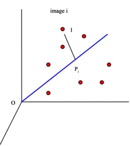
The entire raw data set, in our example, consists of 200,000 images of each 90,000 pixels or a total of 18 × 109 pixel density measurements. In the hyperspace representation, this translates to a cloud of 200,000 points in a 90,000 dimensional hyperspace, again consisting of 18 × 109 co-ordinates. Each co-ordinate corresponds to one of the original pixel densities, thus the hyperspace representation does not change the data in any way. This type of representation is illustrated in Figure 1 for a data set simplified to the extreme, where each image con-sists of just two pixels.
[image:4.595.165.465.413.609.2]The basic idea of the MSA approach is to optimize the orthogonal co-ordinate system of the hyperspace to best fit the shape of the cloud. We wish to rotate (and possibly shift) the co-ordinate system, such that the first axis of the rotated co-ordinate system will correspond to the direction of the largest elongation of the data cloud. In the simplistic (two-pixel images) example of Figure 1, the largest elongation of the cloud is associated with the average density in the two pixels increasing together. That main direction points from the lower left of the illustration (both pixels have low density) to the top right (both pixels high density). The remaining direction is perpendicular to the first one (also indicated in the illustration) but that direction describes only small modula-tions with respect to the main trend of the data set and may be ignored. The power of the MSA approach lies in this data reduction. It allows us to then concentrate on the most important trends and variations found in a com-plex data set and ignore all the other sources of fluctuations (which in EM usually is just noise). We thus enormously reduce the total amount of data into just a few main “principal” components, which show the most significant variations of the data cloud.
Figure 1. Hyperspace representation of an (extremely) simple set of images, each image consisting of only two pixels. Thus, two numbers completely determine each raw image in this minimalistic data set. Each image is fully represented by a single point in a two-dimensional hyperspace. Together, these points form a data “cloud”. The cloud has a shape as indicated in this example. The main purpose of “MSA” approaches is to optimally adapt the co-ordinate system of this hyperspace to the shape of the cloud, as indicated by the blue arrows in this picture. The shape of the data cloud indicates that the largest source of variations in this data set is that of the densities of both pixels increasing together. That single (rotated) direction
Concentrating on the main direction of variations within the data, in the example of Figure 1, reduces the problem from a two-dimensional one to just a one-dimensional problem. This reduction of dimensionality can take dramatic proportions with real EM data sets. In the case of a data set of two hundred thousand images of 300 × 300 pixels, typically some 50 - 200 orthogonal directions suffice to describe the most significant (largest) sources of variations within the data. Each image is then no longer described by the 90,000 density values of its pixels, but rather by just its 50 - 200 co-ordinates with respect to those main directions of variations. This represents a reduction in the dimensionality of the data by more than three orders of magnitude. After this data reduction, it becomes feasible to perform exhaustive comparisons between all images in the data set at a rea-sonable cost. The main orthogonal directions of variations within the data are known as “eigenvectors”; the va-riance that each eigenvector describes is known as the corresponding eigenvalue. Because each eigenvector cor-responds to a point in hyperspace these, in our case, have the character of “image” and are therefore usually re-ferred to as “eigenimages”.
3. Distances and Correlations: The Choice of the Metric
Multivariate Statistical Analysis is all about comparing large sets of measurements and the first question to be re-solved is how to compare them. What measure of similarity one would want to use? The concepts of distances and correlations between measurements are closely related, as we will see below. Different distance and asso-ciated correlation criteria are possible depending on the metric one chooses to work with. We will start with the simplest and most widely used metric: The classical Euclidean metric.
3.1. Euclidean Metrics
The classical measure of similarity between two measurements F(a) and G(a) is the correlation or inner product
(also known as the covariance) between the two measurement vectors:
( ) ( )
(
)
1, FG
a p
C F a G a
=
=
∑
⋅ (1)The summation in this correlation between the two vectors is over all possible values of a, in our case, the p
pixels of each of the two images being compared. (This summation will be implicit in all further formulas; impli-cit may also be the normalization by 1/p). Note that when F and G are the same (F = G), this formula yields the variance of the measurement: the average of the squares of the measurement:
( ) ( )
(
)
( )
21, 1,
FF VAR
a p a p
C F a F a F a F
= =
=
∑
⋅ =∑
= (1a)Closely related to the correlation is the Euclidean squared distance between the two measurements F and G:
( )
( )
(
)
22 FG
D =
∑
F a −G a (2)The relation between the correlation and the Euclidean distance between F and G becomes clear when we work out Equation (2):
( )
( ) ( )
( )
(
)
2 2 2
2
FG
D =
∑
F a − ⋅F a ⋅G a +G a (3)( )
( )
( ) ( )
2 2
2
F a G a F a G a
=
∑
+∑
− ⋅∑
⋅2
VAR VAR FG
F G C
= + − ⋅ (4)
In other words, the Euclidean square distance between the two measurements F and G, is a constant (the sum of the total variances in F and in G, FVAR+ GVAR, respectively, minus twice CFG, the correlation between F and G.
Thus correlations and Euclidean distances are directly related in a simple way: the shorter the distance between the two, the higher the correlation between F and G; when their distance is zero, their correlation is at its maxi-mum. This metric is the most used metric in the context of multivariate statistics; it is namely the metric associ-ated with Principal Components Analysis (PCA, see below). Although this is a good metric for signal processing in general, there are some disadvantages associated the with use of pure Euclidean metrics.
multiply one of the measurement, say F(a), with the constant value of “10”. A multiplication of a measurement by such a constant does not change the information content of that measurement. However, the correlation value
CFG between the measurements F and G (Equation (1)) will increase by a factor 10. The Euclidean square
dis-tance will, after this multiplication, be totally dominated by the FVAR term which will then be one hundred times
larger than the corresponding GVAR term in (Equation (4)).
A further problem with the Euclidean Metric (and with all other metrics discussed here) is the distorting in-fluence that additive constants can have. Add a large constant to the measurement F and G, and their correlation (Equation (1)) and Euclidean distance (Equations (2)-(4)) will be fully dominated by these constants, leaving just very small modulations associated with the real information content of each of F and G. A standard solution to these problems in statistics is to correlate the measurements only after subtracting the average and normalis-ing them by the standard deviation of each measurement. The correlation between F and G thus becomes:
( )
(
)
(
( )
)
(
)
FG AV SD AV SD
C =
∑
F a −F F ⋅ G a −G G (5)( )
( )
(
)
2F′ a G a′
=
∑
− (5’)( )
(
)
(
)
(
(
( )
)
)
( )
(
)
(
( )
)
(
)
2 2 2 2FG AV SD AV SD
AV SD AV SD
D F a F F G a G G
F a F F G a G G
= − + −
− ⋅ − ⋅ −
∑
∑
∑
(6)( )
( )
( ) ( )
2 2
2
F′ a G′ a F a G a′ ′
=
∑
+∑
− ⋅∑
⋅ (6’)This normalisation of the data is equivalent to replacing the raw measurements F(a) and G(a) by their nor-malised versions
F a
′
( )
andG a
′
( )
:( )
(
( )
AV)
SDF a′ = F a −F F (7)
( )
(
( )
AV)
SDG a′ = G a −G G (8)
These substitutions thus render the Euclidean metrics correlations and distances (Equations (5) and (6)) to exactly the same form as the original ones (Equations (1) and (2)).
3.2. Pretreatment of the Data
Interestingly, it is a standard procedure to “pretreat” EM images prior to any processing and during the various stages of the data processing and this routine is, in fact, a generalisation of this standard normalisation in statis-tics discussed above. During the normalisation of the molecular images [30] one first high-pass filters the raw images to remove the very low spatial frequencies. These low spatial frequencies are associated mainly with long-range fluctuations in the image density on a scale of ~20 nm and above. Such long-range fluctuations are not directly related to the structural details we are interested in, and they often interfere with the alignment pro-cedures traditionally required to bring the images in register.
The high-pass filtering is often combined with a low pass filter to remove some noise in the high-frequency range, again, trying to reduce structure-unrelated noise. These high spatial frequencies, however, although very noisy, also contain the finest details one hopes to retrieve from the data. For a first 3D structure determination, it may be appropriate to suppress the high frequencies. During the 3D structural refinements, the original high frequency information in the data may later be reintroduced. The overall filtering operation is known as “band- pass” filtering.
not “zero” but rather the average density in the image, a value which is not normally experimentally available. The band-pass filtering allows one to concentrate on a range of structural details sizes that are important at the current level of processing or analysis. It has a clear relation to the standard normalization of measurements, as in Equations (7) and (8), but has a much richer range of applications.
3.3. Chi-Square Metrics (χ
2-Metrics)
As was mentioned above, the first applications of MSA techniques in electron microscopy [11][12] focused on “correspondence analysis” (CA) [13]-[15] which is based on Chi-square metrics (χ2-metric). Chi-square dis-tances are good for the analysis of histogram data, that is per definition positive. The χ2 correlation and distance are, respectively:
( )
( )
(
)
FG AV AV
Cχ =
∑
F a F ⋅G a G (9)and,
( )
( )
(
)
22
FG AV AV
Dχ =
∑
F a F −G a G (10)With the χ2-metrics, the measurements F and G are normalized by the average of the measurements:
( )
( )
AVF a
′
=
F a F
(11)( )
( )
AVG a
′
=
G a G
(12)Substituting the normalized measurements (11) and (12) into formulas (9) and (10) brings us again back to the standard forms (1) and (2) for the correlation and distance.
Why this normalisation by the average? Suppose that of the 15 million inhabitants of Beijing, 9 million own a bicycle, and 6 million do not own a bicycle. Suppose also that we would like to compare these numbers with the numbers of cyclists and non-cyclists in Cambridge, a small university city with only 150,000 inhabitants. If the corresponding numbers for Cambridge are 90,000 bicycle owners versus 60,000 non-owners, then the χ2 dis-tance (10) between these two measurements is zero, in spite of the 100 fold difference in population size be-tween the two cities. This metric χ2 is thus well suited for studying histogram-type of information.
Interestingly, with the χ2-distance, the idea of subtracting the average from the measurements in already “built in”, and leads to identically the same distance (10) as can be easily verified:
( )
(
)
(
( )
)
(
)
( )
(
)
(
( )
)
(
)
( )
( )
(
)
2 2 2 2 1 1FG AV AV AV AV
AV AV
AV AV
D F a F F G a G G
F a F G a G
F a F G a G
χ = − − −
= − − − = −
∑
∑
∑
(10a)This illustrates that the χ2-metrics are oriented towards an analysis of positive histogram data, that is, towards data were the role of the standard deviation FSD and of the average FAV in Equation (7), are both covered by the
average of the measurement FAV. Although this leads to nice properties in the representation of the data (see
be-low) problems arise when the measurements F(a) are not histogram data but rather a non-positive signal. The normalisation by the average FAV rather than by the standard deviation FSDmay then lead to an explosive
be-haviour of
F a F
( )
AV when the average of the measurements gets close to zero.3.4. Modulation Metrics
microscopy, and a new “modulation”-oriented metric was introduced to circumvent the problem [33]. With the modulation distance, one divides the measurements by their standard deviation (“SD”). The correlation value and the square distance with modulation metrics thus becomes:
( )
( )
(
)
m FG SD SD
C =
∑
F a F ⋅G a G (13)and,
( )
( )
(
)
22
m FG SD SD
D =
∑
F a F −G a G (14)With
( )
(
)
21
SD
F F a
p
=
∑
(15)and,
( )
(
)
21
SD
G G a
p
=
∑
(16)The MSA variant with modulation distances we call “modulation analysis”, and this MSA technique shares the generally favourable properties of CA, yet, as is the case in PCA, allows for the processing of zero-aver- age-density signals.
4. Matrix Formulation: Some Basics
We have thus far considered an image (or rather any measurement) as a vector named F(a) or as a vector named
G(a). We want to study large data sets of n different images (say: 200,000 images), each containing p pixels (say 90,000 pixels). For the description of such data sets we use the much more compact matrix notation. For com-pleteness, we will repeat some basic matrix formulation allowing the first time reader to remain within the nota-tion used here.
4.1. The Data Matrix
In matrix notation we describe the whole data set by a single symbol, say “X”. X stands for a rectangular array of values containing all n × p density values of the data set (say: 200,000 × 90,000 measured densities). The matrix
X thus contains n rows, one for each measured image, and each row contains the p pixel densities of that image:
1,1 1,2 1,3 1, 2,1 2,2 2,3 2,
,1 ,2 ,3 , p
p
n n n n p
x x x x
x x x x
X
x x x x
= (17)
4.2. Correlations between Matrices
This notation is much more compact than the one used above because we can, for example, multiply the matrix
X with a vector G (say an image with p pixels) to yield a correlation vector C as in:
1,1 1,2 1,3 1, 1
1
2
,1 ,2 ,3 ,
,1 ,2 ,3 ,
p
i i i i p i
p
n n n n p n
x x x x c
g g
x x x x
X G c
g
x x x x c
⋅ = ⋅ = (18)
The result of this multiplication X G⋅ is a vector C, which has n elements, and any one element of C, say Ci
(
,)
1,i i a a
a p
c x g
=
=
∑
⋅ (19)This sum is identical to the correlation or inner product calculation presented above for the case of the Euclidean metrics (Equation (1)). Explained in words: one here multiplies each element from row i of the data matrix X with the corresponding element of vector G to yield a vector C, the n elements of which are the corre-lations (or inner products or “projections”) of all the images in the data set X with the vector G.
An important concept in this matrix formulation is that of the “transposed” data matrix X denoted as XT:
1,1 2,1 ,1
1,2 2,2 ,2
T
1,3 2,3 ,3
1, 2, ,
n n n
p p n p
x x x
x x x
x x x
X
x x x
= (20)
In XT, the transposed of X, the columns have become the images, and the row have become what first were the columns in X. Similar to the multiplication of the matrix X with the vector G, discussed above, we can calculate the product between matrices, provided their dimensions match. We can multiply the X with XT because the rows of X have the same length p as the columns of XT:
T
n
A
= ⋅
X X
(21a)This matrix multiplication is like the earlier one (18) of the (n × p) matrix X with a single vector G (of length
p) yielding a vector C of length n. Since XT is itself a (p × n) matrix the inner-product operation is here applied to each column of XT separately, and the result thus is an (n × n) matrix An. Note that each element of the matrix A is the inner product or co-variance between two images (measurements) of the data set X. The n diagonal ele-ments of An contain the variance of each of the measurements. (The variance of a measurement is the co-vari-
ance of an image with itself). The sum of these n diagonal elements is the total variance of the data set, that is, the sum of the variances of all images together, and it is known as the trace of A. The matrix A is famous in multivariate statistics and is called the “variance co-variance matrix”. Note that we also have in the conjugate representation (see below):
T
p
A =X ⋅X (21b)
4.3. Transposing a Product of Matrixes
Note that the matrix An (Equation (21a)) is square and that its elements are symmetric around the diagonal:
therefore its transposed is identical to itself (
A
nT=
A
n). The transposed of the product of two matrices is equal to the product of the transposed matrices but in reverse order as in:(
)
T T TG H⋅ =H ⋅G . We thus also have:
(
) ( )
T TT T T T T
n n
A =A = X X⋅ = X ⋅X =X X⋅ (21c)
4.4. Rotation of the Co-Ordinate System
In the introduction of the MSA concepts above, we discussed that we aim at rotating the Cartesian co-ordinate system such that the new, rotated co-ordinate system optimally follows the directions of the largest elongation of the data cloud. Like the original orthogonal co-ordinate system of the image space, the rotated one can be seen as a collection of, say q orthogonal unit vectors (vector with normalized length of 1), and the columns of matrix U:
1,1 2,1 ,1
1,2 2,2 ,2
1,3 2,3 ,3
1, 2, ,
q q q
p p q p
u u u
u u u
u u u
U
u u u
= (22)
project the p-dimensional image vectors, stored as the rows in the data matrix X, onto the unit vectors stored as the columns of the matrix U:
img
C =X U⋅ (23) Each row of the n × q matrix Cimg again represents one full input image but now in the rotated co-ordinate
system U. We happen to have chosen our example of n = 200,000 and p = 90,000 such that n > p. That means that for the rotated co-ordinate system U we can have a maximum of p columns spanning the p-dimensional space (in other words: q ≤ p). The size of Cimg will thus be restricted to a maximum size of n × q. We may
choose to use values of q smaller than p, but when q = p, the (rotated) co-ordinate matrix Cimg will contain all the
information contained in the original data matrix X.
4.5. An Orthonormal Co-Ordinate System
In an orthonormal co-ordinate system the inner products between the unit vectors spanning the space is always zero, apart from the inner product between a unit vector and itself, which is normalised to the value 1. This or-thonormality can be expressed in matrix notation as
T
q
U ⋅ =U I (24)
We have already seen the matrix U above (equation (22)); the matrix UT is simply the transposed of U. The matrix Iq is a diagonal matrix, meaning that it only contains non-zero element along the diagonal from the top-left
to the lower right of this square matrix. All these diagonal elements have a unity value implying that the columns of U have been normalized.
4.6. The Inverse of Unit Vector Matrix U
The normal definition of the inverse of a variable is that the inverse times the variable itself yields a unity result. In matrix notation, for our unit vector matrix U, this becomes:
1
q
U− ⋅ =U I (25)
The unit matrix Iq is again a diagonal matrix: its non-zero elements are all 1 and are all along the diagonal
from the top-left to the lower right of this square matrix. The “left-inverse” of the matrix U is identical to its transposed version UT (see above). We will thus use these as being identical below. We will use for example: (UT)−1 = U.
4.7. Conjugate Representation Spaces
It may already have been assumed implicitly above, but let us emphasise one aspect of the matrix representation explicitly. Each row of the X matrix represents a full image, with all its pixel-values written in one long line. To fix our minds, we introduced a data matrix with 200,000 images (n = 200,000) each containing 90,000 pixel densities (p = 90,000). This data set can thus be seen a data cloud of n points in a p-dimensional “image space”. An alter-native hyperspace representation is equally valid, namely, that of a cloud of p points in an n-dimensional hyper space. The co-ordinates in this conjugate n-dimensional space are given by the columns of matrix X rather than its rows.
The columns of matrix X correspond to specific pixel densities throughout the stack of images. Such col-umn-vectors can therefore be called “pixel-vectors”. The first column of matrix X thus corresponds to the top-left pixel density throughout the whole stack of n input images. Associated with the matrix X are two hyper-spaces in which the full data set can be represented: 1) the image-space in which every of the n images is represented as a point. This space has as many dimensions as there are pixels in the image; image-space is thus p-dimensional. The set of n points in this space is called the image-cloud; 2) the pixel-space in which every one of the p pixel-vectors is represented as a single point: pixel-space is n-dimensional. The set of p points in this space is called the pixel-vector-cloud or short: pixel-cloud. (This application-specific nomenclature will obviously change depend-ing on the type of measurements we are processdepend-ing.)
analyses in both conjugate spaces are fully equivalent and they can be transformed into each other through “transition formulas”. There is no more information in one space than in the other! In the example we chose n = 200,000 and p = 90,000. The fact that n is larger than p means that the intrinsic dimensionally of the data matrix X
here is “p”. Had we had fewer images n than pixels p in each image, the intrinsic dimensionally or the rank of X
would have been limited to n. The rank of the matrix is the maximum number of possible independent (non-zero) unit vectors needed to span either pixel-vector space or image space.
5. Mathematics of MSA Data Compression
The mathematics of the PCA eigenvector eigenvalue procedures have been described in various places (for ex-ample in [14][15][33]). We here try to follow what we consider the best of earlier presentations with a bit of a further personal twist. We want to find a unit vector that best describes the main direction of elongation of the data cloud. “Best” here means finding a direction which best describes the variance of the data cloud.
5.1. MSA: An Optimization Problem
Let direction vector “u” be the vector we are after (Figure 2); the variance of image I that is described by a vec-tor u is the square of the length of the projection of image I onto the vector u, that is OPi2. If the vector u is to maximize the variance it describes of the full data cloud, we need to maximize
∑
OPi2 where the sum is over all the n images in the data cloud. In doing so, we are also minimizing∑
IPi2, the sum of the square distances of all images to the vector u, making this a standard least-square minimization problem. We have seen above (Equation (18)) how to calculate the inner product of the full data matrix X and a unit vector u.i
[image:11.595.205.424.379.626.2]c = X u⋅ (26)
The sum
∑
OPi2 we want to maximize is the inner product of this resulting co-ordinate vector with itself or: Ti i
c
⋅
c
. We thus can write this as the variance we want to maximise:2 T T T T
i i i p
OP =c ⋅ =c u ⋅X ⋅ ⋅ =X u u ⋅A ⋅u
∑
(27)Let u1 be the unit vector that maximises this variance and let us call that maximised variance λ1. (We will see below how this maximum is actually calculated). We then have for this variance maximizing vector:
T
1 p 1 1
u ⋅A u⋅ =
λ
(28a)Since u1 is a unit vector we have (see above) the additional normalisation condition: T
1 1
1
u
⋅ =
u
(28b)The data matrix has many more dimensions (keyword “rank”) than can be covered by just its main “ eigen-vector” u1, which describes only λ1of the total variance of the data set. (As mentioned above, the total variance of the data set is the sum of the diagonal elements of A, known as its trace). We want the second eigenvector u2
to optimally describe the variance in the data cloud that has not yet been described by the first one u1. We thus
want:
T
2 p 2 2
u ⋅A u⋅ =
λ
(28c) While, at the same time, u2is normalized and perpendicular to the first eigenvector, thus:T
2 2
1
u
⋅ =
u
(28d)and,
T
1 2
0
u
⋅
u
=
(28e)5.2. Eigenvector Equation in Image Space
It now becomes more appropriate to write these “eigenvector eigenvalue” equations in full matrix notation. The matrix U contains eigenvector u1 as its first column, u2as its second column, etc. The matrix Λis a diagonal matrix with as its diagonal elements the eigenvalues λ1, λ2, λ3, etc.:
T T T
p
U ⋅X ⋅ ⋅ =X U U ⋅A U⋅ = Λ (29a)
with the additional orthonormalization condition:
T
q
U ⋅ =U I (29b)
The eigenvector eigenvalue Equation (29a) is normally written as:
T
X ⋅ ⋅ = ⋅ ΛX U U (29c)
which is the result of multiplying both sides of Equation (29a) by U =
( )
UT −1.5.3. Eigenvector Equation in the Conjugate Pixel-Vector Space
Let the eigenvectors in the space of the columns of the matrix A be called V (with v1 the first eigenvector of the space as its first column, v2 the second column of the matrix V, etc.). The eigenvector equation in this “pixel- vector” space is very similar to the one above (Equation (29a)):
T T T
n
V ⋅ ⋅X X ⋅ =V V ⋅A V⋅ = Λ (30a) With the additional orthonormalization condition:
T
q
V ⋅ =V I (30b)
T
n
X X⋅ ⋅ =V A V⋅ = ⋅ ΛV (30c) It is obvious that the total variance described in both image space and pixel-vector space is the same since the total sum of the squares of the elements of all row of matrix X is the same as the total sum of the squares of the elements of all columns of matrix X. The intimacy of both representations goes much further, as we see will be-low.
5.4. Transition Formulas
Multiplying both sides of the eigenvector Equation (29c) from the left with the data matrix X yields:
(
T)
(
) (
)
X X⋅ ⋅ X U⋅ = X U⋅ ⋅ Λ (31)
This equation is immediately recognised as the eigenvector equation in the conjugate space of the pixel vec-tors, Equation (30c) with the product matrix (X·U) taking the place of the eigenvector matrix V. Similarly, mul-tiplying both sides of the eigenvector equation (30c) from the left with the transposed data matrix XT yields
(
T) (
T) (
T)
X ⋅X ⋅ X ⋅V = X ⋅V ⋅ Λ (32)
Again, this equation is immediately recognised as the eigenvector equation in image space (Equation (29c)) with the product matrix XT·V taking the place of the eigenvector matrix U. However, the product matrices X·U
and XT·V are not normalised the same way as are the eigenvector matrices V and U, respectively. The matrix U, is normalised through UT·U = Iq (Equation (29b)), but the norm of the corresponding product matrix XT·V is
given by eigenvector Equation (30a):
(
VT⋅X) (
⋅ XT⋅V)
= Λ. In order to equate the two we thus need to scale the product matrix by the square root of the eigenvalues:T 1 2
U=X ⋅ ⋅ ΛV − (33) and, correspondingly:
1 2
V = X U⋅ ⋅ Λ− (34) These important formulas are known as the transition formulas relating the eigenvectors in image space (p space) to the eigenvectors in pixel-vector space (n space).
5.5. Co-Ordinate Calculations
We mentioned earlier that the co-ordinates of the images in the space spanned by the unit vectors U are the product of X and U (Equation (23)); we now expand on that, using transition formulas (34) and (33):
1 2
img
C =X U⋅ = ⋅ ΛV (35)
and their pixel-vector space equivalents
T 1 2
pix
C =X ⋅ = ⋅ ΛV U (36)
5.6. Eigen-Filtering/Reconstitution Formulas
We have seen that the co-ordinates of the images with respect to the eigenvectors (or any other orthogonal co-ordinate system of p space) are given by: X·U = Cimg(Equation (23)). Multiplying both sides of that equation
from the right by UT (a q × p matrix) yields:
T
img
X∗=C ⋅U (37a)
Using Equation (34) we can also write this equation as
1 2 T
The reason for using a “*” to distinguish X* from the original X, is the following: we are often only interested in the more important eigenvectors, assuming that the higher eigenvectors and eigenvalues are associated with ex-perimental noise rather than with real information we seek to understand. Therefore we may restrict ourselves to a relatively small number of eigenvectors, or restrict ourselves to a value for q, of say, 50. The formulas can now be used to recreate the original data (X) but restricting ourselves to only that information that we consider important.
6. Mathematics of MSA with Generalized Metrics
We have introduced various distances and correlation measures earlier, but in discussing the MSA approaches we have so far only considered conventional Euclidean metrics.
6.1. The Diagonal Metric Matrices
N
and
M
We have discussed above that Euclidean distances are not always the best way to compare measurements and that it may be sometimes better to normalize the measurements by their total (χ2 distances) or by their standard deviation (Modulation distance). In matrix notation let us introduce an n × n diagonal weight matrix N that has as its diagonal elements 1/wi, where wiis, say, the average density of image xi, or the standard deviation of that
image (row i of the data matrix X). Note that then the new product matrix X′ = N·X will have rows xi′ which will have all its elements divided by the weight wi. We then calculate the associated variance-covariance matrix:
(
)
(
)
T T
p
A′ = X′ ⋅X′= X ⋅N ⋅ N X⋅ (38)
Interestingly, now all the elements of this variance co-variance matrix are normalized by the specific weights
wi for each original image as required for the correlations we discussed above for the χ2 metrics (Equation (9))
or the modulation metrics (Equation (13)).
Similarly, we can introduce a diagonal (p × p) weights matrix M in the conjugate space with diagonal ele-ments 1/wj, where wj is, the average density of pixel-vector xj, or the standard deviation of that pixel vector
(column j of the data matrix X). Note that then the product matrix X' = X·M will have columns x′j which will have all its elements divided by the weight wj. Lets us now combine these weight matrices in both conjugate
spaces into a single formulation. Instead of the original data matrix X we would actually like to use a normalized version X' which relates to the original data matrix X as follows:
X′ =N X M⋅ ⋅ (39)
and its transposed:
T T
X′ =M X⋅ ⋅N (40)
6.2. Pretreatment of X with Metric Matrices
N
and
M
Let us now substitute these in to the PCA eigenvector eigenvalue Equation (29c):
T
X′ ⋅X U′⋅ = ⋅ ΛU
Leading to:
T
M X⋅ ⋅ ⋅ ⋅ ⋅N N X M U⋅ = ⋅ ΛU (41) with the additional (unchanged) orthonormalization constraint (29b):
T
q U ⋅ =U I
With the N and M normalisations of the data matrix X, nothing really changed with respect to the mathematics of the PCA calculations with Euclidean metrics discussed in the previous paragraphs. All the important formulas can be simply generated by the substitution above (Equation (39)). For example, the co-ordinate Equation (35) becomes:
1 2
img
C =X U′⋅ = ⋅ ⋅N X M U⋅ = ⋅ ΛV (42)
procedures of the MSA analysis are not affected by pretreatment of the data (although the results can differ sub-stantially).
The normalisation of the data by N and M allow us to perform the eigenvector analysis from a perspective of χ2 distances or that of modulation distances. This normalisation means that, in the 9,000,000 bicycle example for χ2 distances, the measurements for Beijing and Cambridge fall on top of each other which is what we wanted.
However, the fact that the weight of the measurement for Beijing is 100 times higher than that for Cambridge will be completely lost with this normalisation! That means that even for the calculation of the eigenvectors and eigenvalues of the system, the weight of Cambridge contribution remains identical to that of Beijing.
In standard (not normalised PCA), the contribution of Beijing to the total variance of the data set to the ei-genvalue/eigenvector calculations would be 1002 =10,000 times higher than that of Cambridge, thus distorting the statistics data set. (Squared correlation functions in general suffer from this problem [34]). It was this distor-tion of the correladistor-tion values that prompted the introducdistor-tion of the normalisadistor-tion matrices N and M in the first place. However, with the full compensation of the standard deviations of total averages through the N and M
matrices we may thus have overdone what we aimed to achieve.
6.3. MSA Formulas with Generalized Metrics in “p Space”
A more balanced approach than either the pure PCA approach or the total normalisation of the data matrix can be achieved by concentrating our efforts on a partially normalised data matrix X′
1 2 1 2
X′ =N ⋅ ⋅X M (43a) and its transposed:
T 1 2 T 1 2
X′ =M ⋅X ⋅N (43b) Substituting these in to the classical PCA eigenvector-eigenvalue equation yields:
T
X′ ⋅X U′⋅ ′=U′⋅ Λ (44a)
1 2 T 1 2 1 2 1 2
M ⋅X ⋅N ⋅N ⋅ ⋅X M ⋅U′=U′⋅ Λ (44b) with the additional (unchanged) orthonormalization constraint
T
q
U′ ⋅U′=I (44c) By then substituting 1 2
U′ =M ⋅U we obtain the eigenvector-eigenvalue equation:
(
) (
)
1 2 T 1 2 1 2 1 2
M ⋅X ⋅ ⋅ ⋅N X M ⋅ M ⋅U = M ⋅U ⋅ Λ (45)
This is equivalent to (multiplying left and right hand side of the equation from the left by M−1/2) the eigenvec-tor-eigenvalue equation for generalised metrics [14][15][33]:
T
X ⋅ ⋅ ⋅N X M U⋅ = ⋅ ΛU (46a) However, by substituting 1 2
U′ =M ⋅U, (and equivalently in the conjugate space 1 2
V′ =N ⋅V) we
deliber-ately choose the co-ordinate system itself to reflect the different weights of the columns and rows of the data matrix and the orthonormalization condition now rather becomes:
(
T 1 2) (
1 2)
Tq
U ⋅M ⋅ M ⋅U =U ⋅M U⋅ =I (46b)
6.4. MSA Basic Formulas with Generalized Metrics in “n Space”
Equivalently, we obtain the eigenvector-eigenvalue equation in the conjugate space as:
(
) (
)
1 2 T 1 2 1 2 1 2
N ⋅ ⋅X M X⋅ ⋅N ⋅ N ⋅V = N ⋅V ⋅ Λ (47a)
or, alternatively, formulated as (the result of a multiplication from the left with (N−1/2) T
X M X⋅ ⋅ ⋅ ⋅ = ⋅ ΛN V V (47b) with the associated orthonormalization condition
(
) (
)
T T 1 2 1 2
q
6.5. Transition Formulas with Generalized Metrics
For deriving the transition formulas we proceed as was done earlier for PCA derivations. Starting from the ei-genvector-eigenvalue Equation (45), and multiplying both sides of this equation from the left with the normal-ized data matrix X′ =
(
N1 2⋅ ⋅X M1 2)
yields:(
) (
)
1 2 T 1 2 1 2 1 2 1 2 1 2
N ⋅ ⋅X M X⋅ ⋅N ⋅ N ⋅ ⋅X M ⋅M ⋅U = N ⋅ ⋅X M U⋅ ⋅ Λ (48)
This last equation, again, is virtually identical to the eigenvector equation in the conjugate space (apart from its scaling):
(
) (
)
1 2 T 1 2 1 2 1 2
N ⋅ ⋅X M X⋅ ⋅N ⋅ N ⋅V = N ⋅V ⋅ Λ (49)
And, again, we have a different normalisation for N1 2⋅V. The latter has a unity norm (see Equation (47c)), whereas N1 2⋅ ⋅X M U⋅ has the norm Λ as becomes clear from multiplying Equation (45) from the left with
T 1 2
U ⋅M yielding:
(
T T 1 2) (
1 2) (
T)
U ⋅M X⋅ ⋅N ⋅ N ⋅ ⋅X M U⋅ = U ⋅M U⋅ ⋅ Λ = Λ (50)
We thus again need to normalise the “transition equation” with Λ−1/2, leading to two transition equations be-tween both conjugate spaces:
1 2
V =X M U⋅ ⋅ ⋅ Λ− (51) and correspondingly:
T 1 2
U=X ⋅ ⋅ ⋅ ΛN V − (52)
6.6. Calculating Co-Ordinates with Generalized Metrics
The calculation of the image co-ordinates in n space as we have seen above (Equation (23)):
img
C′ =X′⋅U′ (23’) With the appropriate substitutions:
(
)
1 2 1 2 1 2
img
C′ =N ⋅ ⋅X M ⋅ M ⋅U (53)
and
1 2
img
C′ =N ⋅ ⋅X M U⋅ (54)
However, these co-ordinates, seen with respect to the eigenvectors U, have a problem: the matrix 1 2
N ⋅ ⋅X M
is only partially normalised with respect to N. With the example of Beijing versus the Cambridge bicycle density, Beijing has a hundred times higher co-ordinate values than Cambridge, while having exactly the same profile. For the generalised metric MSA we thus rather use the co-ordinates normalised fully by N and not just by N1/2
[14][15][33]:
1 2
img
C = ⋅ ⋅N X M U⋅ = ⋅ ⋅ ΛN V (55)
(The right hand side was derived using the transition formula V =X M U⋅ ⋅ ⋅ Λ−1 2 (Equation (51)) multi-plied from the right by Λ1/2.) And we also have, similarly:
T 1 2
pix
C =M X⋅ ⋅ ⋅ =N V M U⋅ ⋅ Λ (56)
7. MSA: An Iterative Eigenvector/Eigenvalue
The algorithm we use for finding the main eigenvectors and eigenvalues of the data cloud is itself illustrative for the whole data compression operation. The IMAGIC “MSA” program, originally written by one of us (MvH) in the early 1980s, is optimised for efficiently finding the predominant eigenvectors/eigenvalues of extremely large sets of images. Here we give a simplified version of the underlying mathematics. Excluded from the mathemat-ics presented here are the “metric” matrices N and M for didactical reasons. The basic principle of the MSA al-gorithm is the old and relatively simple “power” procedure (cf. [35]; also discussed in Wikipedia under “eigen-vector power iteration”). In this traditional approach one multiplies a randomly chosen “eigen-vector r1, through the symmetric variance co-variance matrix A, which will yield a new vector r1′:
1 1
A r⋅ =r′ (57a) This resulting vector is then (after normalisation) successively multiplied through the matrix A again:
1 1
A r⋅ =′ r′′ (57b) and that procedure is then repeated iteratively. The resulting vector will gradually converge towards the first (largest) eigenvector u1of the system, for which, per definition, the following equation holds:
1 u1 A u1
λ ⋅ = ⋅ (58)
Why do these iterative multiplications necessarily iterate towards the largest eigenvector of the system? The reason is that the eigenvectors “u” form a basis of the n-dimensional data space and that means that our random vector r1 can be expressed as a linear combination of the eigenvectors:
1 1 1 2 2 3 3
r =c u +c u +c u + (59) The iterative multiplication through the variance-covariance matrix A will yield for r1 after k iterations (using Equation (58) repeatedly):
1 1 1 1 2 2 2 3 3 3
k k k
k
r
=
c
λ
u
+
c
λ
u
+
c
λ
u
+
(60a)or:
3 3
2 2
1 1 1 1 2 3
1 1 1 1
k k
k k
c c
r c u u u
c c
λ
λ
λ
λ
λ
= + + + (60b)Because λ1 is the predominant eigenvalue, the contributions of the other terms will rapidly vanish
(λ λi 1k 1; i > 1), and these iterations will thus make r1 rapidly converge towards the main eigenvector u1.
The variance co-variance matrix A is normally calculated as the matrix multiplication of the data matrix X and it's transposed, XT:
T
p
A =X ⋅X (61)
As was mentioned above, the data matrix X contains, as its first row, all of the pixels of image 1; its general ith row contains all the pixels of image i. The MSA algorithm operates by multiplying a set of randomly generated eigenvectors (because of the nature of the data also called eigenimages) r1, r2, etc., through the data matrix U and its transposed U' respectively. The variance-covariance matrix Ap is thus never calculated explicitly since
that operation is already too expensive in terms of its massive computational burden. The MSA algorithm does not use only one random starting vector for the iterations, but rather uses the full set of q eigenimages desired and multiplies that iteratively through the data matrix X, similar to what was suggested by [36].
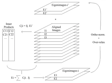
In detail the MSA algorithm works as follows (Figure 3). The eigenvector matrix Uq is first filled with
Figure 3. The iterative MSA eigenvector-eigenvalue algorithm. The program first fills a matrix U with orthonormalised random column number vectors (E1', E2', etc.). This matrix is then multiplied through the data matrix X containing the set of images I1 through In as rows. This multiplication leads to a ma-trix of coefficients C which is then multiplied through the transposed data matrix XT leading to (after normalization) a better approximation of the eigenvector matrix. In essence the algorithm performs a continuous set of iterations through the eigenvector Equation (29a) 1 T
U′′= Λ ⋅− X ⋅ ⋅X U′. (For the
equivalent including the influence of generalized metrics, we have from Equation (46a):
1 T
U′′= Λ ⋅− X ⋅ ⋅ ⋅N X M U⋅ ′).
set. The algorithm converges rapidly (typically within 30 - 50 iterations) to the most important eigenimages of the data set.
An important property of this algorithm is its efficiency for large numbers of images n: its computational re-quirements scale proportionally to n∙p, assuming the number of active pixels in each image to be p. Most eigen-vector-eigenvalue algorithms require the variance-covariance matrix as input. The calculation of the vari-ance-covariance matrix, however, is itself a computationally expensive algorithm requiring computational re-sources almost proportional to n3. (This number is actually: Min (n2p, np2)). The MSA program produces both the eigenimages and the associated eigenpixel-vectors in the conjugate data space as described in [33]. One of the intuitive charms of this fast disk-based eigenvector-eigenvalue algorithm is that it literally sifts through the image information while finding the main eigenimages of the data set. The programs have been used routinely for more than 30 years, on a large number data sets consisting of up to ~1,000,000 individual images.
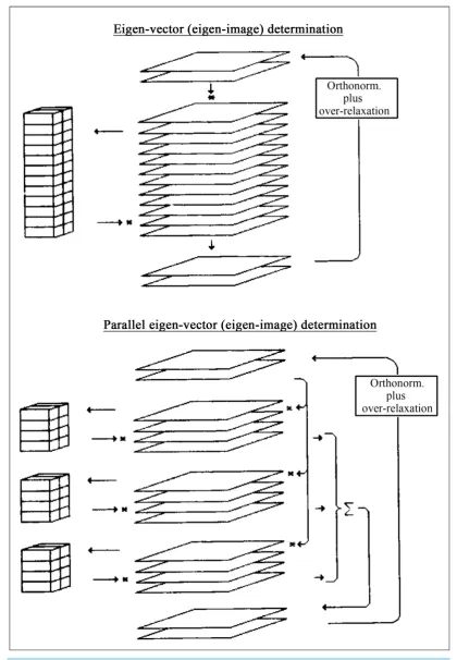
8. Parallelization of the MSA Algorithm
In spite of its high efficiency and perfect scaling with the continuously expanding sizes of the data sets, com-pared to most conventional eigenvector-eigenvalue algorithms, the single-CPU version of the algorithm had be-come a serious bottleneck for the processing of large cryo-EM data sets. The parallelisation of the MSA algo-rithm had thus moved to the top of our priority list. We have considered various parallelisation schemes includ-ing the one depicted in Figure 4; this mapping of the computational problem onto a cluster of computers was indeed found to be efficient.
Figure 4. Parallelisation of the MSA algorithm. Note that for an efficient operation it is essential that the part of the input data matrix X that is of relevance to one particular node of the cluster, is indeed always available on a
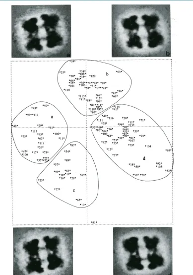
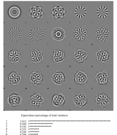
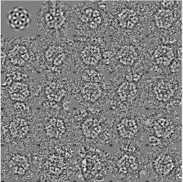
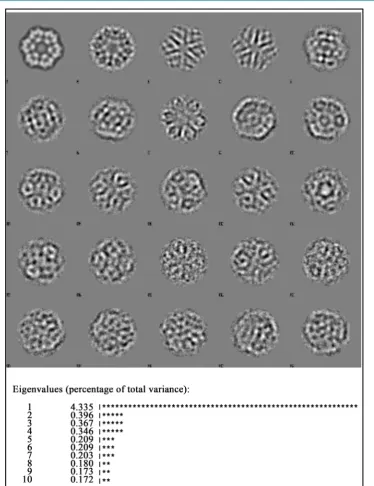
![Figure 6. Symmetry analysis. Some of the ~7300 particles selected au-tomatically from a set of micrographs using the automatic particle pick-ing program PICK_M_ALL (part of the IMAGIC-4D software system [46])](https://thumb-us.123doks.com/thumbv2/123dok_us/7865629.737730/25.595.182.446.358.624/symmetry-analysis-particles-selected-tomatically-micrographs-automatic-particle.webp)