AN IOT BASED FRAMEWORK FOR STUDENTS INTERACTION AND PLAGIARISM DETECTION IN PROGRAMMING ASSIGNMENTS

4850

FAST REPRESENTATION OF FLUID SHEETS WITH GRID

PROJECTION AND CPU-GPU HETEROGENEOUS

COMPUTING

JONG-HYUN KIM1 _{,JUNG LEE}2

1_{Division of Software Application, Kangnam University, Gyeonggi, South Korea}

2_{School of Software, Hallym University, Chuncheon, South Korea}

E-mail: 1_{[email protected],} 2_{[email protected]}

ABSTRACT

We introduce a fluid simulation method using a upsampling-based grid projection and CPU-GPU heterogeneous computing that can explicitly represent and preserve fluid thin sheets. The most important contribution of this paper is that the GPU and grid projection are used to improve the particle-based framework to prevent holes that appear to collapse at thin fluid surfaces or dense points. The proposed framework can handle topology change reliably without numerical diffusion or twisting problems. The anisotropic kernel and PCA (Principal Component Analysis) are performed on the GPU to quickly find the direction of fluid with a thin surface, and CPU-GPU heterogeneous computing technique greatly enhances the efficiency of the candidate position extraction process to calculate the position of a new fluid particle. Our technique is intuitively implemented, allowing for easy parallelization and rapid visualization of the surface of thin sheets of visually detailed water. As a result, we propose a parallel processing framework that can quickly express surface details, such as liquid sheets, that are difficult to represent in traditional particle-based simulations and improve the surface details of the water simulation.

Keywords: CPU-GPU heterogeneous computing, Thin sheets of water, Fluid simulation

1. INTRODUCTION

Representing the turbulence of the detailed fluid generated from the interaction of the fluid and the solid has been an important issue in physics-based simulation. Especially, it is very important to generate and express fine detail when performing fluid animation including turbulence or liquid sheets [13],[14],[17],[18],[19] (refer to figure 1).

Figure 1: Real images of fluid sheets [13],[14]

Adaptive grid and multigrid methods have been widely used to model turbulent flows that are represented in fluid simulations [1],[2]. These methods can temporally express the small detail vortex phenomena by solving the Navier-Stokes equation in a grid space with higher resolution. However, if the vortex deviates from the high-resolution grid space, it becomes difficult to preserve its detailed motion. To solve this problem, hybrid framework techniques have been introduced that express the motion of small turbulence [3],[18].

Since the Smoothed Particle Hydrodynamics (SPH) technique proposed by Muller et al. [4], there has been much progress in the field of particle-based simulation [20],[21],[22]. Conventional particle-based methods are suitable for bubble or splash animation, but are not sufficient to express the characteristics of a thin fluid because of the oscillation problems caused by the spring force.

4851 actually used because they require large amounts of computation. This paper introduces a new particle-based CPU-GPU heterogeneous framework that preserves the thin features of liquids, such as Eulerian fluid simulations. Our approach is to find out where the thin surface of the fluid disappears and add/remove new particles.

Figure 2: APIC coupled simulation of elastoplastic frozen yogurt and elastic cloth where coupling is

achieved using MPM method

We use the Fluid-implicit-particle (FLIP) method as the underlying fluid solver [5] (refer to figure 3), which preserves the surface of the liquid that is thin and disappears by adding new fluid particles. The added particles are removed when they enter a location where the thin features of the fluid can not be extracted (e.g, deep water region).

Figure 3: Stanford bunny is simulated as water and as sand

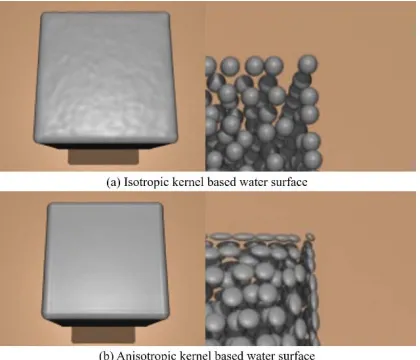
This study is also influenced by the anisotropic kernel method proposed by Yu and Turk [6]. Their method employs the stretch and orientation of the particles to perform PCA using the location of the surrounding particles and, as a result, to restore sharp, smooth fluid surfaces (refer to figure 4). We use the GPU-based solution to perform the PCA and use this stretch as a basis for determining whether to insert fluid particles [27].

2. RELATED WORK

The latest liquid surface tracking techniques can be categorized into two approaches: Implicit and Explicit. The level-set method proposed by Osher

and Sethian is one of the most widely used implicit methods [26]. The level-set method computes the distance function from the nearest surface position in each grid node and implicitly defines the surface where the distance value is zero. This method has been improved and modified in various aspects over the years. Enright et al. [25], Wang et al. and Mihalef et al. placed a Lagrangian particle to prevent numerical loss. Solving this implicit method in a high-resolution grid can increase the overall fluid detail. However, even with this approach, it is still not enough to capture the thin film-like features of the fluid.

Figure 4: Comparison between the surface reconstruction using isotropic kernel (a) and anisotropic

kernels (b)

Hirt and Nichols proposed a volume of fluid (VOF) technique that uses the ratio of fluids to all cells to efficiently represent discontinuous interfaces [7]. Other methods have been proposed over the past several decades in various research areas, such as medical imaging and fluid dynamics [8] (refer to figure 5).

Figure 5: Dropping viscoelastic balls in an Eulerian fluid simulation

4852 used because it is difficult to cope with self-intersection or complex topology transformation. This problem can be solved by resampling neighboring grid positions, but it complicates the algorithm because we must consider all the various complex situations.

Figure 6: Simulation of three-dimensional film boiling

The particle-based approach is not as complicated in terms of algorithms because it does not retain the vertex of the mesh and expresses the surface of the fluid using only particles, as in the explicit approaches [4],[20],[21],[22]. The splittable particle based approach used in this paper belongs to the category of adaptive particle method. Our method and this method are designed to keep the thin film-like characteristics of the fluid constant, while the only difference is that we reduce the computational cost while maintaining the visual detail of the fluid by sampling the particles with different sizes (refer to figure 7).

Figure 7: Water splash by our method. (a): A visualized splash with particles, (b): A thin generated by our

method

3. OUR FRAMEWORK

The proposed method is a CPU-GPU heterogeneous framework that generates and

maintains thin features of fluids using FLIP-based three-dimensional fluid particles. The algorithm is performed in the following order.

I. Step1(GPU) Particle density calculation, surface particle extraction

II. Step2(GPU) Calculating direction of particles, finding pair of particles, extracting candidate position of newly added particles III. Step3(CPU Parallel) Optimizing candidate

position

IV. Step4(CPU Serial) Adding and removing new particles

V. Step5(GPU) Velocity calculation through grid projection

VI. Step6(CPU Parallel) Advection of fluid particles

VII.Step7(GPU) Reconstruction of fluid surfaces

3.1 Sections and Subsections

The proposed method is based on the method of Ando et al. [15],[16], which maintains a thin film of fluid. First, the distribution of particles is analyzed using an anisotropic kernel. To extract the orientation of the particles we first calculate the average covariance 𝐶 per particle as follows (refer to equation 1).

𝐶 ∑ _{∑ ,} , (1)

Where 𝑑 is the initial distance between the fluid particles, and 𝛼 is the variable that controls the initial distance 𝑑 .

𝑝 ∑_∑ ,

, (2)

𝑊 𝑟, ℎ 1

‖ ‖

, 0 ‖𝑟‖ ℎ,

0, 𝑜𝑡ℎ𝑒𝑟𝑤𝑖𝑠𝑒 (3)

We calculate the eigenvectors and eigenvalues for the particle distribution using the covariance matrices 𝐶 computed using the above formulas and SVD (singular value decomposition). We extract the stretch and orientation of adjacent particles from these values.

𝐶 𝑒 𝑒 𝑒

𝜎 𝜎

𝜎 𝑒 𝑒 𝑒

(4)

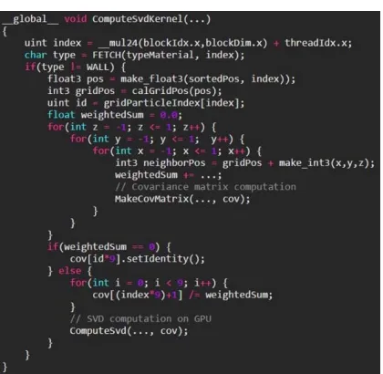
4853 surface are extracted by inspecting 𝜎 𝛼 𝜎 , where 𝛼 is a threshold value for determining the degree of thickness. Figures 8 and 9 are pseudo codes with the CUDA kernel that calculate the process up to the SVD calculation using the density of the fluid particle and the covariance matrix. This process corresponds to Step1 and Step2.

Figure 8: Computing of particle density in GPU

Figure 9: Computation of covariance matrix and singular value decomposition in GPU

The pseudo code shown in Figure 8 roughly classifies surface particles using the density values of the fluid particles, and the pseudo code of Figure 9 calculates the covariance matrix using the distance from adjacent particles. Finally, SVD is used to calculate eigenvectors and eigenvalues using GPU-based parallel programming, and finally the results of the extracted thin particles are shown in Figure 10.

Figure 10: Selected thin particles from water particles (thin particles are colored violet and lie on the outer

edge of the fluid body)

3.2 Extraction and Optimization of Candidate Position

The extracted thin particles are used to add new particles to the hole part. We find (i, j), which is the pair of particles used to fill the hole. 𝑝 𝑝 /2, which is the center position of the pair, is stored for use as a candidate position for splitting, and finally a pair satisfying all of the following conditions is finally selected.

𝛼 𝑑 𝑝 𝑝 𝛼 𝑑 (5a)

∑ 𝑊 𝑝 , 𝛼 𝑑 0 (5b)

𝑝 𝑝 ∙ 𝑢 𝑢 0 (5c)

Where 𝛼 and 𝛼 are constants that control the minimum and maximum distance between candidate positions and u is the particle velocity. Equation 5a checks that the two particles are at an appropriate distance from each other. Equation5b examines whether there are no fluid particles around the candidate position, in other words, a sparse region, to determine if it is appropriate to add new particles within the radius 𝛼 . Equation 5c confirms that the distance between a pair of fluid particles increases over time. As a result, the intermediate position of the pair satisfying all the above conditions is stored in S without duplication.

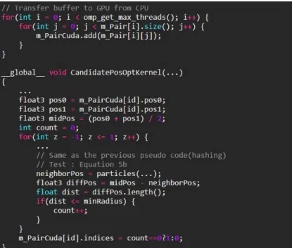
4854 Figure 11 shows a pseudo code for calculating the candidate positions using a CPU-based parallel module. This process corresponds to Step 3. In the method of Ando et al. [15],[16], it takes a long time to calculate because it finds a pair satisfying all three conditions for all fluid particles. In order to efficiently process this, we divide it into a CPU-GPU heterogeneous parallel framework. Figure 5 is a pseudo code for finding a pair satisfying Equations 5a and 5c. In this paper, we use OpenMP for CPU-based parallel processing and generate a pair buffer by the maximum number of threads (omp_get_max_threads()) provided by the CPU. Pairs satisfying the conditions 5a and 5c are stored in the pair buffer corresponding to each thread index (m_Pair[omp_get_thread_num()]).

Figure 12: Optimization of candidate position in GPU

Since a large number of candidate pairs are extracted from the pair sets calculated in this process, Equation 5b takes a long calculation time. We perform GPU-based parallel processing to efficiently calculate this process (refer to figure 12)

Figure 13: Computing S buffer in GPU

Finally, we pass the pair buffer (m_PairCuda) computed on the GPU to the CPU (m_Pair[i][]). Figure 13 is a pseudo code that performs this process and consequently forms an S buffer.

3.3 Inserting and Removing Particles

It is not appropriate to add new fluid particles where the candidate particles are densely arranged. Therefore, this chapter describes how to filter out unnecessary particles and add only a minimal number of particles to preserve liquid sheets. I is a list of extracted information of the final candidate particles, 𝐼 is the first position value in S :

𝐼 𝑎𝑟𝑔𝑚𝑖𝑛∈𝑺 𝜌 𝑠 (6)

Where 𝜌 is the density of the 𝑗th particle. We calculate 𝐼 from S and then delete the candidate particles that are in radius 𝛼 𝑑 from the surrounding particles of 𝑠 . We then search for particles outside the radius 𝛼 from the surrounding particles of 𝑠 and add them to 𝑁 . Finally, the closest particle 𝑠 of the particles in 𝑁 is added to

𝐼 (refer to equation 7).

𝐼 𝑎𝑟𝑔𝑚𝑖𝑛∈ 𝑠 𝑠 (7)

Equation 7, used to search for particles, can be computed as : 𝐼 𝑠𝑒𝑎𝑟𝑐ℎ 𝐼 . This means that

𝐼 can be calculated in the same way, and

𝐼 , 𝐼 , … , 𝐼 . If the search fails and there are no candidates satisfying the condition, Equation 6 is used instead.

Based on the above, the fluid particle is divided into two particles and its properties are linearly interpolated. The velocity u and density ρ mapped to the grid are calculated as follows :

𝑢 𝑥 ∑_{∑ ,}, (8)

𝜌 𝑥 ∑ 𝑚 𝑊 𝑝 𝑥, 𝛼 𝑑 (9)

Here, 𝛼 is a weight value for velocity u, and 𝑊

is a kernel function as follows :

𝑊 𝑟, ℎ ‖ ‖ , 0 ‖𝑟‖ ℎ,

0, 𝑜𝑡ℎ𝑒𝑟𝑤𝑖𝑠𝑒 (10)

In this study, as in Ando's method, fluid particles are removed when one of the following conditions is satisfied (refer to equations 11 and 12).

𝜌 𝛼 𝜌 and 𝜎 𝜎 𝜎 (11)

4855 Where 𝛼 is the maximum density value and 𝛼 is the minimum distance value between the fluid particles. The fluid particles are removed if they meet Equations 11 and 12, and the mass of the removed particles is added back to the original fluid particles before splitting, thus preserving the total mass. The process of adding and deleting fluid particles is a serial structure so that 𝐼 is processed after 𝐼 is processed. So we treated it in the same way as the algorithm proposed by Ando et al. [15],[16]. In the next section, we describe how to calculate the velocity efficiently using the grid projection.

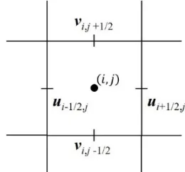
3.4 Grid Projection for Pressure Solver

Mapping velocity to coarse grid : To map from particle to coarse grid, we propose a normalized spline kernel method to map the intermediate fine grid velocity 𝑢 to a coarse grid and then obtain the coarse velocity 𝑢 . To map the velocity field 𝑢

stored in the fine grid to the coarse grid field 𝑢 , we use the distance-weight average function as follows:

𝑢_, ∑_∑ ,

, (13)

Where 𝑑 𝑥 𝑥, is the distance between

the position of 𝑚 fine grid velocity 𝑢 and the position of the coarse grid velocity 𝑢, , and the

spline kernel 𝑊 is calculated as:

𝑊 𝑟, ℎ ℎ 𝑑 , 𝑟 ℎ,

0, 𝑜𝑡ℎ𝑒𝑟𝑤𝑖𝑠𝑒 (14)

Where the influence radius ℎ is a constant value as 0.5 times the size of a coarse grid.

Making coarse grid incompressible : After obtaining the down-sampled velocity field 𝑢 in the coarse grid, we use a coarse projection operation to make the field divergence-free. And we handle the object boundary in the coarse projection step.

We handle the boundary mismatch between the coarse and the fine grids using a variational framework. Instead of using the standard discretization of the Laplacian operator, we use a mass-weighted 7-point Laplacian stencil to discretize the Poisson equation. Then, the final linear system is solved using the preconditioned conjugate gradient method to obtain the pressure result. We then subtract the pressure gradient from 𝑢 (refer to Equation 15).

𝑢∗ _{𝑢 ∆𝑡 ∇𝑝 (15)}

Where the result 𝑢∗ _{satisfies the incompressibility of}

fluid on the coarse grid.

Figure 14: Reconstruction field refined by a factor of m.

Mapping back to fine grid : After obtaining the divergence-free velocity field 𝑢∗ _{in the coarse grid,}

we need to map this field back to a fine grid. We propose a new upsampling method for reconstructing a fine divergence-free field from a coarse divergence-free field. The key to this method is to refine the grid cell (i, j) using factor 𝑚. As shown in Figure 14, the values of the fine grid cell (i, j) are calculated as follows using

𝑢 , 𝑢 , 𝑣 , 𝑣 known from the coarse grid and upsampling methods.

𝑢 _{/ ,} (16)

𝑢 _{/ ,} (17)

𝑣_{, /} (18)

𝑣_{, /} (19)

Remember the discrete divergence in two dimensions is :

∇ ∙ 𝑢 , / ,_∆ / , , /_∆ , /

(20)

We simply substitute the values on Equations 16-19 into the divergence formula, Equation 20, and get the following equation :

∇ ∙ 𝑢 _,

∆ (21)

4856 ∆ ∆ 0 (22)

Therefore, Equation 22 equals to zero, which means the divergence on the fine grid is free.

3.5 Surface Reconstruction

In order to recover the surface of the fluid, we use the SVD value used to extract the thin particles. In this paper, the anisotropic feature of SVD is reflected in the algorithm of Yu et al. [6] and the surface of the fluid is reconstructed in detail. The level-set of particles is calculated as follows :

𝜙 𝑥 min ‖ 𝐺 𝑝 𝑥 ‖ (23)

Here, 𝐺 represents a transformation matrix for the fluid particle i, and its detailed form is as follows :

𝐺

𝑒 𝑒 𝑒

𝜎

0

0

0

0

0

0

𝑒 𝑒 𝑒

(24)

Here, 𝑘 is a scale constant, and 𝜎 is suggested within a certain range to preserve the greatest stretching. For a more detailed explanation, we recommend that you refer to the work of Yu et al [6]. We used a GPU based Marching Cubes algorithm and set the minimum stretching value to be less than the grid spacing so that thin fluid surfaces can be represented well.

4. IMPLEMENTATION

This study was implemented in the following environment : Intel i7-7700k 4.20GHz CPU 32GB RAM, and NVIDIA GeForce GTX 1080 Ti Graphics card. The FLIP-based fluid solution was used as the underlying water simulation and the GPU-based preconditioned conjugate gradient method was used as the numerical solver to calculate the fluid pressure [10]. In the FLIP grid, all the momentum was stored using the Staggered Marker-and-Cell method [11] and an additional grid was used for surface reconstruction.

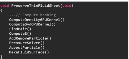
Figure 15: Pseudo-code of our framework

We also used the boundary particle method proposed by Akinci et al. [12] for the collision processing of water and solid. Figure 15 shows the pseudo code of the algorithm that preserves the characteristics of the thin fluid proposed in this paper. Time-consuming processes, such as transferring momentum between grids and particles or calculating pressure, are computed in CPU and GPU-based parallel frameworks

5. RESULTS

In order to analyze the proposed framework in various ways, we compared our methods in three scenarios.

Figure 16: Thin fluid sheets by our method

Figure 16 shows a drop of spherical liquid from above, using 300,000 fluid particles and setting the time-step to 0.006. The result is 8 times faster, yielding the same results as the CPU-based technique of Ando et al. [15],[16] As shown in Figure 8, we quickly and clearly expressed the thin film and filaments of the fluid as the spherical liquid collides with the main fluid body.

4857 surface of the fluid compared to Laplacian smoothing, but some loss of thin fluid sheets still occurs (refer to figure 17c).

Figure 17: Comparison results : dropping a liquid sphere

On the other hand, our method minimizes the problem of thin fluid sheet loss and expresses the surface of the fluid in detail, and the scene is created faster than the conventional methods through the grid projection and GPU-based framework.

Figure 18: Deformable pumpkins thrown from various directions

The detailed features of the thin surface of the fluid can be easily seen in coupling scenes where solid and fluid collide. To prove that the proposed method works well in the coupling scene, we cast a deformable object into the fluid to naturally create a splash phenomenon (refer to figure 18). As you can see in the picture, the moment the pumpkin model touches the water, the appearance of the water crown

is well expressed. In addition, when the water contacts the transparent wall boundary, the fluid surface is clearly visible without breaking. In this case, 1.2 million fluid particles were used and 12 times as fast as that produced by Ando’s method [15],[16]. In addition, a water pouring scene was created to show where thin particles could actually be added to maintain the thin surface of the fluid when using the proposed method (refer to figure 18).

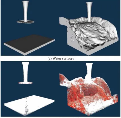
Figure 19: Water pouring off a box

This result shows a thin surface of the fluid that is expressed as water falls from the top to the bottom due to water pouring (refer to figure 19). The red particles are newly added thin particles, which represent thin films of fluid. This result can be made in the same way as in Ando et al. [15],[16], but the proposed method shows about 9 times faster than Ando's method.

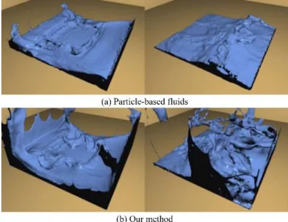
4858 Figure 20 is a scene in which water is stirred with a box-shaped rod, capturing the detail of the fluid well, just like any other scene. In this scene, we used about 1 million fluid particles. As you can see in the figure, the liquid sheets are well represented in the red box. Our method showed about 4 times faster performance than Ando's method due to grid projection and CPU-GPU heterogeneous computing.

Figure 21: Results with Ando’s method [15][16] (inset image : our method)

Figure 21 compares the results of our technique (inset images) with the Ando's method [15],[16] of representing liquid sheets, and this paper produced similar results visually when compared with the previous technique. (refer to figures 16 and 19 for more detailed results).

Table 1 summarizes the experimental results of this paper. Since the number of particles varies to preserve fluid thin sheets every frame, the average number is added to the table. In addition, we used a higher resolution grid in the surface reconstruction process to detail the thin fluid sheets. Compared to the previous techniques [15],[16], the performance is improved by about 4 to 12 times when all the results are expressed in similar visual quality. In addition, the performance was not only improved in certain scenes, but was also stably improved in all scenes.

Table 1: Size of our example scenes and computational time (Avg. : average, Num. : number, Res. : resolution,

Perform. : performance)

Fig. Avg.

num. of particles

Grid res. (Pressure solver)

Grid res. (Surface reconstruction)

Perfor m. gain

16 1m 128^3 200^3 8

17 1m 128^3 200^3 8

18 1m 128^3 200^3 12

19 650k 128^3 128^3 9

20 1m 128^3 256^3 4

6. DISCUSSION AND CONCLUSIONS

We proposed a grid projection and a CPU-GPU heterogeneous framework to efficiently represent

thin films of fluids. Generally, the GPU adds the process of copying data from the CPU to the GPU for parallel computation and copying back from the GPU to the CPU to reflect the computed results again. To reduce this unnecessary process, we used a CPU-based parallel scheme where the amount of computation was not large. Our method showed improved performance results in all scenes. The performance of the existing techniques we refer to is largely influenced by the number of fluid particles generated in the initial scene and the number of thin particles created accordingly. As a result, the performance of the proposed method is significantly improved as the number of total particles increases.

A limitation of the proposed method is that it is difficult to produce high-resolution scenes due to the limitation of memory capacity. To represent a thin film of fluid, more particles are required than the number of fluid particles set in the initial scene, and a large number of thin particles can be generated per frame. In the future, we plan to study how to efficiently manage the memory and produce large-scale fluid simulations.

REFRENCES:

[1] Dobashi, Y., Matsuda, Y., Yamamoto, T., Nishita, T., A fast simulation method using overlapping grids for interactions between smoke and rigid objects. Computer Graphics Forum, Vol. 27, No. 2, 2008, pp. 477 486.

[2] Losasso, F., Gibou, F., Fedkiw, R., “Simulating water and smoke with an octree data structure”. ACM SIGGRAPH, 2004, pp. 457 462.

[3] Selle, A., Rasmussen, N., Fedkiw, R., “A vortex particle method for smoke, water and explosions”. ACM SIGGRAPH, 2005, pp. 910-914.

[4] Mattias. M., D. Charypar, Gross. M., “Particle-based fluid simulation for interactive applications”, Proceedings of the 2003 ACM SIGGRAPH/Eurographics Symposium on Computer Animation, 2003, pp. 154-159.

[5] Zhu, Y., Bridson, R., “Animating sand as a fluid”. ACM SIGGRAPH, 2005, pp. 965-972.

[6] Yu, J., Turk, G., “Reconstructing surfaces of particle-based fluids using anisotropic kernels”. ACM SIGGRAPH, Vol. 32, No. 1, 2013, pp. 5:1-5:12.

4859 [8] Wojtan C., Thurey N., Gross M., Turk G,

“Deforming meshes that split and merge”. ACM SIGGRAPH, 2009, pp. 76:1–76:10.

[9] C. Dyken and G. Ziegler, “GPU-accelerated data expansion for the marching cubes algorithm”, In Proceeding PGU Technology Conference, 2010, pp. 115–123.

[10] R. Li and Y. Saad, “GPU-accelerated preconditioned iterative linear solvers”, The Journal of Supercomputing, Vol. 63, No. 2, 2013, pp. 443–466.

[11] F. H. Harlow and J. E.Welch, “Numerical calculation of time-dependent viscous incompressible flow of fluid with free surface”, The Physics of Fluids, Vol. 8, No. 12, 1965, pp. 2182–2189.

[12] N. Akinci, J. Cornelis, G. Akinci, and M. Teschner, “Coupling elastic solids with smoothed particle hydrodynamics fluids”, Computer Animation and Virtual Worlds, Vol. 24, No. 3-4, 2013, pp. 195–203.

[13] Rivas, A., Altimira, M., Sanchez Larraona, G., & Ramos, J. C., “Analysis of liquid-gas flow near a fan-spray nozzle outlet”. In Conference on Modelling Fluid Flow, 2006, pp. 6-9. [14] Lhuissier, Henri, and Emmanuel Villermaux.

“Destabilization of flapping sheets: The surprising analogue of soap films”. Comptes Rendus Mecanique, Vol. 337, 2009, pp. 469-480. [15] R. Ando and R. Tsuruno, “A particle-based

method for preserving fluid sheets”, In Proceedings of the 2011 ACM SIGGRAPH/ Eurographics Symposium on Computer Animation. 2011, pp. 7–16.

[16] R. Ando, N. Thurey, and R. Tsuruno, “Preserving fluid sheets with adaptively sampled anisotropic particles”, IEEE Transactions on Visualization and Computer Graphics, Vol. 18, No. 8, 2012, pp. 1202–1214. [17] Jong-Mo Hong, T. Shinar, and R. Fedkiw, “Wrinkled flames and cellular patterns”, ACM Transactions on Graphics, Vol. 26, No. 3, 2007. [18] Doyub Kim, Seung Woo Lee, Oh-young. Song, and Hyeong-Seok Ko, “Baroclinic turbulence with varying density and temperature”, IEEE Transactions on Visualization and Computer Graphics, Vol. 18, No. 9, 2012, pp. 1488–1495. [19] Doyub Kim, Oh-young. Song, and Hyeong-Seok Ko, “Stretching and wiggling liquids”, ACM Transactions on Graphics, Vol. 28, No. 5, 2009, pp. 120:1–120:7.

[20] P. Goswami, P. Schlegel, B. Solenthaler, and R. Pajarola, “Interactive SPH simulation and

rendering on the GPU”, In Proceedings of the 2010 ACM SIGGRAPH/Eurographics Symposium on Computer Animation, 2010, pp. 55–64.

[21] T. Harada, S. Koshizuka, and Y. Kawaguchi, “Smoothed particle hydrodynamics on GPUs”, In Computer Graphics International, 2007, pp. 63–70.

[22] H. Yan, Z. Wang, J. He, X. Chen, C. Wang, and Q. Peng, “Real-time fluid simulation with adaptive SPH”, Computer Animation and Virtual Worlds, Vol. 20, No. 2-3, 2009, pp. 417– 426.

[23] Jiang, C., Schroeder, C., Selle, A., Teran, J. and Stomakhin, A., “The affine particle-in-cell method”. ACM Transactions on Graphics, Vol. 34, No. 4, 2015, pp.51.

[24] Stomakhin, A., Schroeder, C., Chai, L., Teran, J. and Selle, A., “A material point method for snow simulation”. ACM Transactions on Graphics, Vol. 32, No. 4, 2013, pp.102.

[25] D. Enright, R. Fedkiw, J. Ferziger, and I. Mitchell, “A hybrid particle level set method for improved interface capturing”, Journal of Computational Physics, Vol. 183, No. 1, 2002, pp. 83–116.

[26]S. Osher and J. A. Sethian, “Fronts propagating with curvature-dependent speed: algorithms based on hamilton-jacobi formulations”, Journal of Computational Physics, Vol. 79, No. 1, 1988, pp. 12–49.

[27] S. Lahabar and P. Narayanan, “Singular value decomposition on GPU using CUDA”, In IEEE Parallel & Distributed Processing, 2009, pp. 1-10.

[28] G. Tryggvason, B. Bunner, A. Esmaeeli, D. Juric, N. AlRawahi, W. Tauber, J. Han, S. Nas, and Y.-J. Jan, “A front racking method for the computations of multiphase flow”, Journal of Computational Physics, Vol. 169, No. 2, 2001, pp. 708–759.