A Splitting Method for the Benjamin Bona Mahoney Equation Using WENO Scheme

2018 International Conference on Physics, Computing and Mathematical Modeling (PCMM 2018) ISBN: 978-1-60595-549-0

A Splitting Method for the Benjamin-Bona-Mahoney

Equation Using WENO Scheme

Ji ZHANG, Xu QIAN*, Yun-rui GUO and Song-he SONG

College of Science and State Key Laboratory of High Performance Computing, National University of Defense Technology, Changsha, 410073

*Corresponding author

Keywords: Benjamin-Bona-Mahoney equation, Discontinuous solution, Weighted essentially non-oscillatory method, Runge-Kutta method.

Abstract.The Benjamin-Bona-Mahoney equation can be split into a system of an elliptic equation and an ordinary differential equation (ODE). For the elliptic equation, we use a classical finite difference weighted essentially non-oscillatory (WENO) scheme. For the ODE, the third order explicit Runge-Kutta method is employed to discretize the time derivative. Due to the WENO reconstruction, the splitting method shows an excellent ability in capturing the formation and propagation of shock peak on solutions. The numerical simulations for asymptotic solution of the BBM equation illustrate the capability of the method.

Introduction

In this paper, we consider a nonlinear, dispersive equation naturally arising in shallow water theory, most concisely exemplified by a version of the Benjamin-Bona-Mahoney (BBM) equation[1], also known as the regularised long wave equation

ut + uux = uxxt , (1)

for a real function u(x, t) of two variables x and t. The original BBM equation, which contains an additional linear convective term ux, is an important model for the description of unidirectional

propagation of weakly nonlinear, long waves in the presence of dispersion. It first appeared in a numerical study of shallow water undular bores[2], and later was proposed in [3] as an analytically advantageous alternative to the Korteweg-de Vries(KdV) equation

ut + uux = -uxxx . (2)

In the context of the shallow water waves, the BBM and KdV equations (1) and (2) are reduced, normalised versions of corresponding asymptotic models derived from the general Euler equations of fluid mechanics using small amplitude, long wave expansions. If δ˂˂1 is the ratio of the undisturbed depth to a typical wave length and ε˂˂1 is the ratio of a typical wave amplitude to the undisturbed depth, then asymptotic KdV and BBM equations occur under the balance ε~δ2 accordingly[4,5], and can be used interchangeably within their common domain of asymptotic validity[6].

Despite all that, the mathematical properties of the BBM and KdV equations are highly different. The KdV equation (2) is known to be integrable via the inverse scattering transform and to possess an infinite number of conservation laws. However, the BBM equation (1) does not enjoy full integrability and has just three independent conservation laws. Nonetheless, well-posedness of initial value problems for both equations has been established in the Sobolev spaces Hs(with s > 0 for BBM[7], s > - 3

As a numerical and mathematical model, the BBM equation yields more satisfactory short-wave behaviour, due to the regularisation of the unbounded growth in frequency, phase and group velocity values presenting in the KdV equation. In particular, this enables less strict timestepping in numerical schemes for the BBM equation. Indeed, linearising (1) with a constant

0: ( , ) 0 ( )

i

uu u x t u ae kxt , we obtain the dispersion relation

0( ; 0) 0 2.

1

k

k u u

k

  

 ₍₃₎

The phase and group velocities are

2

0 0

0

2 2 2

1

, .

1 (1 )

p g k

u k

c c

k k k

 _ 

    

  ₍₄₎

We can see that 0,cp _and cg _{are bounded as functions of the wave number} k_{, in contrast to}

their counterparts for the KdV equation with dispersion relation 0 0

3

u k k

   _{. The rational form}

of BBM dispersion (3) indicates its non-local character. Moreover, the dynamics of linear dispersive equations with discontinuous initial data exhibit distinct qualitative structure depending upon bounded or unbounded dispersion behaviour for large k [9].

In this paper, we give the WENO scheme to the problem with shock. The WENO methodologies[17,18] are high order numerical approximations for solving PDEs which may contain discontinuities, sharp gradient regions and other complex solution structures. The splitting method is effective and high-efficiency to solve discontinuous solutions of the BBM equation, which can reduce the computational complexity. Firstly, we emphasize the construction of the WENO finite difference scheme for the BBM equation. Then the second order difference method is presented for the discretization of the dispersion term. In addition, the proposed method is tested a number of numerical problems with shock. Finally concluding remarks are given.

High Order Optimized Difference WENO Method

Using the inverse operator I xx_{, which} I _{is unit matrix, we split the BBM equation into a}

system of a elliptic equation and an ODE. The process can now be reformulated with more detail as follows.

From (1), a routine computation gives rise to

(I _xx)u_tuu_x 0.

(5)

Multiplying both sides of (5) by

1

(I _xx)

, we obtain

1

( ) 0.

t xx x

u   I uu 

(6)

By substituting

1

( _xx) _x

p  I  uu

into (6), the following equations are obtained.

0,

t u  p

(7)

- xx ( ) .x

p p  f u

(8)

where

2

1 ( )

2

x

f u  u

.

0 1 N ,

L x x x L

     

which are called by cell centers, with so-called nodes given by

1 2 2 i i h x x   

, where

2L h

N



is the uniform grid interval. The spatial finite difference discretization of (8) can be written as

( ) ( ),

i xx i x i

p p x  f x

(9)

with pi  p x t( , )i _{. A conservative finite difference formulation for the BBM equation requires}

high order consistent numerical fluxes at the cell nodes in order to form the flux differences across

the uniformly spaced cells. We implicitly define the numerical flux function g x( ) as

2 2

1

( ) ( )d ,

h x

h x

f x g

h  

 



_

such that the spatial derivative in (9) is exactly approximated by the following conservative finite difference method

1 1 2 2

1

( ) ,

i xx i

i i

p p x g g

h  

 

  _  _

  ₍₁₀₎

where

1 1

2 2

( )

i i

g g x

  

.

The classical (2r-1)-order WENO method uses a (2r-1)-points global stencil S2r-1, which is subdivided into r substencils S0,S1,…,Sr-1,with each substencil containing r grid points. So the

(2r-1)-order approximations of

1 2 i g



are computed by (2r-1)-points polynomial interpolations. Therefore (9) can be reformulated as

1 1 2 2

1 _{ˆ ˆ}

( ) ,

i xx i

i i

p p x f f

h  

 

  _  _

  ₍₁₁₎

where 1 2 ˆ i f 

is a (2r-1)-order approximations of

1 2 i g  .

For an ordinary flux f u( ), it can be split into f u( ) f ( )u f ( )u

 

  _{, satisfying} df_du( )u 0



and

d ( )

0 d

f u u



. A simple Lax-Friedrichs splitting is applied as

1

( ) ( ( ) ) 2

f u  f u u

where 

is set as max |u f u( ) |



over the range of u. Thus

1 1 1

2 2 2

ˆ ˆ ˆ

i i i

f f f

    

, where both

1 2 ˆ i f  and 1 2 ˆ i f 

are built through the convex combination of the interpolated values

1 2

ˆ (k )

i f x



and

1 2

ˆ (k )

i f x



respectively. For simplicity, we only do the reconstruction of

1 2 ˆ i f  : 1 1 1 0 2 2

ˆ r _{ˆ ( ),}

k k

i i

k

f  f x

 

 



_ 

(12)

1 1

0 2

ˆ ( ) , 0 , , .

r

k k j i k j

i j

f x c f i N



 

 



_ 

(13)

The Lagrangian interpolation coefficients ckj _{depend on the parameter} k0, ,r1. _The

classic weights k _{are defined as}

1 0

, .

( )

k k

k r k p

k l l d          



(14)

The local smoothness indicators k _{are computed by}

1 2 1 2 2 1 2 1 1

d _{ˆ ( ) d ,}

0,1, , 1. d i i l r _x l

k _x l k

l

h f x x k r

x          _{ }    



_

(15)

The expression of the k _{in terms of the cell values of} f _{are given by[20]}

2 2

0 2 1 2 1

2 2

1 1 1 1 1

2 2

2 1 2 1 2

13 1

( 2 ) ( 4 3 ) ,

12 4

13 1

( 2 ) ( ) ,

12 4

13 1

( 2 ) (3 4 ) .

12 4

i i i i i i

i i i i i

i i i i i i

f f f f f f

f f f f f

f f f f f f

                               

Finally, the central differentiation method is applied for pxx _{in (11). Therefore we can obtain}

the discretization of (8):

1 1

1 1 2

2 2

2 1 _{ˆ ˆ}

, 1, 2, , .

i i i

i

i i

p p p

p f f i N

h h           _  _ 

  ₍₁₆₎

The Third Order Explicit Runge-Kutta Method for the ODE

In this section, we present the time discretization of the ODE (8) with the third order explicit Runge-Kutta method (RK3). According to [21, 22], we can obtain the following formulas:

(1) (2) (1) 1 (2) , 3 1 ( ), 4 4 1 2 ( ). 3 3 n h h n

h h h

n n

h h h

u u tp

u u u tp

u  u u tp

  

   

   

(17) In fact, the Runge-Kutta method is a convex linear combination of the forward Euler method,

which can confirm third-order time precision. Moreover, it follows from (17) that

1 n h u 

can be

obtained by the known

n h u

.

Numerical Examples

( , 0) tanhx, ,

u x A x



    

(18) where the amplitude A>0. Thus, as  0, the initial data converges to a jump from u-A to uA, representing a stationary expansion shock solution to the inviscid Burger’s equation. The uniformly valid asymptotic solution of the initial value problem (1), (18) was given [1] as follows:

( , ) (tanh sgn( )) ( , , ),

1 1

2

A x

u x t x F x t

A t

 



  



(19)

where

,

1

( sgn( )) 2

( , , ) , | |

1 1

2 ,

A x At

A x x

F x t x At

A t

A x At

 





  

 

 



_ 

 



 _

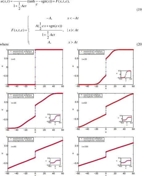
[image:5.593.74.534.175.746.2]

 ₍₂₀₎

Figure 1. The numerical and asymptotic solutions.

ODE(WENO5-RK3). Then we analyse the solution by matched asymptotics using  as the small

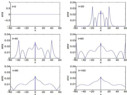
parameter[1]. We show the numerical and asymptotic solutions in Fig.1 with A1, 0.1 which shows that the overall solution transitions accurate. Fig.2 shows the pointwise error between the

numerical and asymptotic solutions. We compute the solutions and errors with x [ 110,110]

and display them in [-60,60] . When xt, the asymptotic solutions are unsmooth, and the dispersion of numerical solutions is great. The solutions are discontinuous at x0. As time goes by, the amplitudes at discontinuous places and the dispersion are smaller.

The numerical solutions have been displayed together with the asymptotic solutions. Compared with the numerical solutions with about x0.009 and t0.01 in [1], the numerical solutions with WENO5-RK3 also successfully reduce the dissipation at the shock position and have similar errors. However, x in this paper is only about 0.06.

Summary

We have proposed a splitting method for the BBM equation containing discontinuous solutions, basing on the WENO reconstruction together with Runge-Kutta method. Firstly we decompose the

BBM equation into an elliptic-ODE system by the inverse operator I xx_{, thus the WENO}

reconstruction can handle the discontinuities appearing in the elliptic equation, while the RK method can easily discretize the derivative in ODE. Therefore, our method not only achieves the expected high accuracy order for smooth solutions, but also accurately captures discontinuities without oscillations. We have carried out extensive numerical computations with various initial conditions, and summarized the results as flowing:

1. The proposed method captures the formation and propagation of shockpeakon with high accuracy.

2. The numerical solutions are displayed together with the asymptotic solutions well.

[image:6.593.91.504.468.777.2]

3. Compared with the numerical solutions in [1], the numerical results with greater x in this paper have similar errors.

Acknowledgement

Supported by the Natural Science Foundation of China under Grant Nos.11571366 and 11501570, and the Open Foundation of State Key Laboratory of High Performance Computing of China Research Fund of NUDT (Grant No. JC15-02-02) and the fund from HPCL.

References

[1]El, Gennady A., M. A. Hoefer, and M. Shearer. Expansion shock waves in regularized shallow-water theory. Proc Math Phys Eng Sci472.2189(2016):20160141.

[2]Peregrine, D. H. Calculations of the development of an undular bore. Journal of Fluid Mechanics 25.2(1966):321-330.

[3]Benjamin, T. B., J. L. Bona, and J. J. Mahony. Model Equations for Long Waves in Nonlinear Dispersive Systems. Philosophical Transactions of the Royal Society of London 272.1220(1972):47-78.

[4]Whitham GB., Linear and nonlinear waves, New York: Wiley; 1974.

[5]Zhongquan, L. V., M. Xue, and Y. S. Wang. A New Multi-Symplectic Scheme for the KdV Equation. Chinese Physics Letters 28.6(2011):060205.

[6]Johnson RS. Camassa-Holm, Kortwegde Vries and related models for water waves, Chin. Phys.

B. 24 (2015), pp. 137-141.

[7]Bona, J L, and N. Tzvetkov. Sharp well-posedness results for the BBM equation. Discrete & Continuous Dynamical Systems - Series A (DCDS-A) 23.4(2012):1241-1252.

[8]Colliander, J., et al. Sharp Global Well-Posedness for KDV and Modified KDV. Journal of the American Mathematical Society 16.3(2003):705-749.

[9]Gong, Chen, and P. J. Oliver. Dispersion of discontinuous periodic waves. Proceedings of the Royal Society A Mathematical Physical & Engineering Sciences 469.2149(2015).

[10]Whitham, G. B. Variational Methods and Applications to Water Waves. Hyperbolic Equations

and Waves. Springer Berlin Heidelberg, 1970:153-172.

[11]Moldabayev D, Kalisch H, Dutykh D., The Whitham equation as a model for surface water waves., Physica D.2015;309:99 107.

[12]Temirkhan Sultanovich, M. Kirane, and Y. F. Tang. Boundary-value problems for differential equations of fractional order.Journal of Mathematical Sciences 194.5(2013):499-512.

[13]Gurevich, A. V, and L. P. Pitaevskii. Nonstationary structure of a collisionless shock wave.Zhurnal Eksperimentalnoi I Teoreticheskoi Fiziki65.2(1974):590-604.

[14]Fornberg, B., and G. B. Whitham. A Numerical and Theoretical Study of Certain Nonlinear

Wave Phenomena. Philosophical Transactions of the Royal Society of London

289.1361(1978):373-404.

[15]El, G. A., M. A. Hoefer, and M. Shearer. Dispersive and diffusive-dispersive shock waves for nonconvex conservation laws. Physics (2016).

[16]Peregrine, D. H. Calculations of the development of an undular bore. Journal of Fluid Mechanics 25.2(1966):321-330.

[17]Jiang G S and Shu C W Efficient implementation of WENO schemes to nonuniform meshes,

[18]Y. Matsuno, Analysis of WENO Schemes for Full and Global Accuracy, 1994 J. Comput. Phys 115 200.

[19]G.S. Jiang, C.W. Shu, Efficient implementation of weighted ENO schemes, J. Comput. Phys.

126 (1996) 202–228.

[20]Y. Xia and Y. Xu, Weighted essentially non-oscillatory schemes for Degasperis–Procesi equation with discontinuous solutions, Annals of Mathematical Sciences and Applications, 2(2017), pp.319-340.

[21]Shu C-W, Osher S., Efficient implementation of essentially non-oscillatory shock-capturing schemes, II, Journal of Computational Physics.1989, 83 (1): 32-78.