A Study of Alternative Single Factor Short Rate Models:
Evidence from United Kingdom (1975-2010)
Romora Edward Sitorus
Sampoerna School of Business, Universitas Siswa Bangsa Internasional, Building D Mulia Business Park, Jl. Letjen MT. Haryono Kav. 58-60, Jakarta, Indonesia, 12780
*Corresponding Author: [email protected]
Copyright © 2014 Horizon Research Publishing All rights reserved.
Abstract This study reviews and compares the
performance of alternative short rate models for one-month UK interbank rate from 1 January 1975 to 1 January 2010 using Generalized Method of Moments (GMM). Controlling for structural break in the data set, this study finds mixed conclusion about the best single factor short rate model. The result also shows that the more restricted model is not preferable to the less restricted one. Moreover, the volatility factor plays more important role than the drift factor in explaining the dynamics of UK short rates.Keywords Short Rate, Interest Rate Modelling,
Structural Break, Generalized Methods of Moments1. Introduction
Various single factor short rate models have been proposed in finance literature. Those classes of short rate models are based on an assumption that changes in interest rates of all maturities are driven by changes in a single underlying random factor. A partial listing of those single-factor models include models created by [29, 11, 12, 22, 26], et cetera. Every development of new short rate models aims to achieve two objectives: first, to get more accurate empirical explanations of the short rate dynamics. Secondly, to find out term structure implication of short rate movements.
In spite of its relative simplicity, single factor short rate models have the abilities to exhibit mean reversion and the capability to allow the volatility to be dependent on the interest rate. Practitioners still use single-factor short rate model despite the availability of multi-factor models such as affine term structure [15] and [25] especially if practitioners would like to value derivatives depending on one maturity, for example caps, or options with early exercise features such as Bermudan or American options [37]. Compared to multi-factor models, single factor short rate models are preferable by practitioners because short rate models are quick to implement and fast to run for calibration. Thus, this
comparison study limits the comparison of interest rate within single factor diffusion framework, unlike [4] and [36] who incorporates more flexible diffusion specification.
The recent literature of short rate models has shown various different conclusions about short rate dynamics. For instance, [1] and [38] find the evidence of nonlinear drifts in the short rate movement. Pritsker [33], however, investigates the finite-sample properties of Aït-Sahalia’s nonparametric and shows that upon accounting for the high persistence in interest rates, the nonlinearity of drift become statistically insignificant. Brenner [9] and Andersen and Lund [2] argue that stochastic volatility/GARCH models are useful to capture conditional heteroskedasticity of interest rates. Moreover, Gray [7], Ang and Bekaert [3] and Jiang and Yan [23] implement regime-switching and jump models and suggest that those models are helpful to fit short-term rate processes with volatility clustering, especially the excess kurtosis and heavy tails of short rates. Conversely, Hong and Li [20] investigate affine models of the Euro dollar rate and suggest that even sophisticated models (including GARCH, regime switching, and jumps) may still not adequately capture interest rate dynamics.
The most recent literature shows that one particular model may not always fit all the short-term rate process. Variety of different conclusions in the literature regarding certain short rate model’s viability can be attributed to the application of different specification test and sample data. Indeed, many short rate comparison analyses have been performed with varying choice of data sets. Bali and Wu [4], for instance, assert that high-frequency data on federal funds rate and Eurodollar rates are not good proxies for true short rate because of its spurious microstructure effects and noise characteristics, respectively. Furthermore, Sam and Jiang [34] argue that while increasing sampling frequency is important for the identification of the short rate process, it is the increase in sampling period that is crucial for the identification of the drift function. In light of those findings, this study examines single factor short rate model using daily UK market-based short rate over a long sample period between 1975 and 2010.
available extensively, there are very limited studies written about the comparability of the models. Chan, Karolyi, Longstaff, and Sanders [10] (hereafter CKLS [10]) is the first study that develop general framework to estimate and investigate a range of different single factor short rate models. Since their paper, other studies have attempted to compare the special cases of short-term risk model such as Tse [40]. Moreover, Bliss and Smith [7] re-examines CKLS [10] results and underline the importance of the regime-shift/structural break in the model interplay. They argue that by redefining regime shift period to the period of “Fed Experiment” between October 1979 and September 1982, they could find evidence that contrast with CKLS [10] results. Fed Experiment is an event where the Federal Reserve Board announced that it would focus more on monetary aggregates and less on interest rate levels as a means of fight historically high inflation. Gray [17] asserts that Fed Experiment period cannot be explained in single regime model because it causes the model to become misspecified.
This study attempts to fix structural break issue in CKLS [10] framework by combining the approach of CKLS [10] with Sanders and Unal [35] to investigate United Kingdom (UK) short rate dynamics. Through this approach, the article provides more robust results insights about the empirical interest rate dynamics. Specifically, this study divides the UK short rate (1975-2010) in the sample into two sub-periods: the period prior to the Black Wednesday (16 September 1992) period and the period aftermath. Black Wednesday is selected as a break point event because it marks the beginning of UK exchange rate regime change from European Exchange Rate Mechanism. That particular event was immediately followed by the decision of Central Bank of United Kingdom to proceed with inflation targeting policy. The policy event created a significant shift in the monetary policy and the behavior of term structure of UK interest rates [5].
In the context of United Kingdom, this article investigates several issues as follows: which is the best single factor short rate models to explain short rate dynamics for UK data? , what is the most important parameter in one-factor models that describe UK short rate movement? how stable is each parameter in various single factor short models prior and after structural shift in UK interest rate regimes.
The remainder of this paper is organized as the following: Section 2 describes the data, section 3 explains the methodology, and section 4 provides the results and discussion. Finally, this study offers the conclusions in section 5.
2. Data Description
Following Nowman and Sorwar [31], this study uses daily one-month UK interbank middle rate in to proxy the short rate. Following the example of Brenner, Harjes, and Kroner [9], this study particular employs the nominal short rate data starting from 1 January 1975 to 30 July 2010. It is assumed that there are 252 trading days and 52 trading weeks a year. All interest rate is converted into annualized rate. Daily short rate data is taken from Datastream Thompson Reuters.
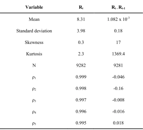
Table 1. Summary statistics
Variable Rt Rt - Rt-1
Mean 8.31 1.082 x 10⁻³
Standard deviation 3.98 0.18
Skewness 0.3 17
Kurtosis 2.3 1369.4
N 9282 9281
ρ1 0.999 -0.046
ρ2 0.998 -0.16
ρ3 0.997 -0.008
ρ4 0.996 -0.016
ρ5 0.995 0.018
Means, standard deviations and autocorrelations of daily one-month interbank middle rate in United Kingdom (1975-2010). The variable rt
denotes the short rate. Rt-rt-1 denotes the rate changes from observations. ρj
denotes the autocorrelation coefficient of order j. N represents the number of observations
Table 1 shows that skewness of level data of short rate and its difference are different from zero and positive, therefore the data is not normal and skewed to the right. Moreover, the kurtosis is less than 3, meaning that the distribution is flatter than normal distribution.
[image:2.595.311.553.216.435.2]Panel A. Level rate of one-month UK Interbank rate Panel B. Yield Change of one-month UK Interbank rate
Figure 1. Level and yield change of daily one-month UK interbank rate
3. Methodology
CKLS [10] uses econometric framework to compare alternative short rate models with the following stochastic differential equation (SDE):
𝑑𝑑𝑑𝑑= (𝛼𝛼+𝛽𝛽𝑑𝑑)𝑑𝑑𝑑𝑑+𝜎𝜎𝑑𝑑𝛾𝛾𝑑𝑑𝑑𝑑 (1)
Where 𝑑𝑑 denotes the interest rate level, t is time and Z is the Brownian motion. Moreover, α,β,σ, and γ are the estimated parameters. In this specification, 𝛼𝛼+𝛽𝛽𝑑𝑑 is a drift and 𝜎𝜎 is the scale factor for the volatility of unexpected interest rate changes. The parameter γ is the constant elasticity of variance with respect to interest rate level. Treepongkaruna and Gray [39] showed that parameter -𝛼𝛼/𝛽𝛽 represent the long-run mean of the interest rate. Thus, for large values of 𝛽𝛽, the short rate responds more sensitively to deviation of the mean.
The general specification in equation (1) encompasses multiple short rate models as listed below:
1. Merton dr = αdt + σdZ 2. Vasicek dr = ( α + βr )dt + σdZ 3. CIR-SR dr = ( α + βr )dt + σ r1/2dZ 4. Dothan dr = σ rdZ
5. GBM dr = βrdt + σ rdZ 6. Brennan- Schwartz dr = (α + βr )dt + σ rdZ 7. CIR-VR dr = σ r3/2 dZ
The corresponding parameter restrictions for those models are further summarized in Table 2. CKLS [10] put different restriction in each parameters of equation (1) to differentiate one model to the others.
Model 1 in table 2 is simply a stochastic process characterized by a Brownian motion with a drift used in Merton [29]. Moreover, model 2 is used by Vasicek [41] to derive a general form of the term structure of interest rates by following Ornstein-Uhlenbeck process.
Model 3 is used by Cox, Ingersoll and Ross [12] using square root process (CIR SR). In this model, the prices and stochastic characteristics of any contingent claims such as bond are derived endogenously. It takes into account the main factors that assume rational expectation and maximizing behavior such as anticipations, risk aversion, alternative, and preferences about the timing of
consumption.
Seven short-rate rate models can be nested in generalized model of CKLS [10] as shown below:
Table 2. Parameter Restrictions on Short Rate Models
Model α β σ γ
1. Merton 0 0
2. Vasicek 0
3. CIR-SR 1/2
4. Dothan 0 0 1
5. GBM 0 1
6. Brennan-Schwartz 1
7. CIR-VR 0 0 3/2
Model 4 is used by Dothan [14] to present a valuation formula for default free bonds. The model utilizes a martingale process which is a zero-drift stochastic process. It follows that for a given current yield r, r (t) has a lognormal distribution. Model 5 is Geometric Brownian motion used by Black and Scholes [6]. It is used by to price the option on debt securities. The interest rate is assumed to follow lognormal distributions.
Model 6 is introduced by Brennan and Schwart [8] to value the price of convertible bond. Model 7 is created by Cox, Ingersoll and Ross [11] to value the variable rate loans contracts. This model assumes that all investors have Bernoulli logarithmic utility of consumption.
This study does not include Constant Elasticity of Variance (CEV) model because this paper attempts to specifically investigate CKLS’s finding that interest rate volatility moves proportionally with interest rate level, by controlling the degree of which the interest level influences the volatility changes. Unlike other models, however, CEV model does not explicitly limit γ to any degree.
3.1. Generalized Method of Moments
Following CKLS [10], this study estimates the parameters of the continuous-time model using a discrete-time econometric specification as follows:
0 4 8 12 16 20 24
1980 1985 1990 1995 2000 2005 2010 -8
-4 0 4 8 12
[image:3.595.315.551.312.445.2]rt+1−rt=α+βrt+εt+1 (2)
E[εt+1] = 0 E[εt+12 ] =σ2rt2γ (3) This discrete-time model allows the variance of interest rate to change according to the level of the interest rate in a way that aligns with the continuous-time model. It is important to understand that discretized process in equation (2) and (3) is just an approximation of continuous-time specification.
CKLS [10] tests equation (2) and (3) as a set of over identifying restrictions on a system of moment equations using the Generalized Method of Moments (GMM) of Hansen [18]. This technique has been chosen due to several advantages it possesses. First, GMM approach can still be used even though the interest rate changes is not normal; Second, GMM estimators and their standard errors are consistent even if the disturbances, ε𝑑𝑑+1, are conditionally heterokedastic. Lastly, the GMM technique has also been used extensively in other empirical tests of interest rate models by Gibbons and Ramaswamy [16], Harvey [19], and Longstaff [27].
The estimation of four parameters in CKLS [10] requires us to include four moment conditions in our estimations as follows:
𝑓𝑓𝑑𝑑(𝜃𝜃) =
⎣ ⎢ ⎢ ⎢
⎡ 𝜀𝜀𝜀𝜀𝑑𝑑+1𝑑𝑑+1𝑑𝑑𝑑𝑑 𝜀𝜀𝑑𝑑2+1− 𝜎𝜎2𝑑𝑑𝑑𝑑2𝛾𝛾
�𝜀𝜀𝑑𝑑2+1− 𝜎𝜎2𝑑𝑑𝑑𝑑2𝛾𝛾�𝑑𝑑𝑑𝑑⎦⎥
⎥ ⎥ ⎤
(4)
Where θ ≡(α, β, σ2 and γ)’and 𝜀𝜀
𝑑𝑑+1 =𝑑𝑑𝑑𝑑+1− 𝑑𝑑𝑑𝑑− 𝛼𝛼 −
𝛽𝛽𝑑𝑑𝑑𝑑.
Following GMM procedure, the restriction is specified where𝐸𝐸[𝑓𝑓𝑑𝑑(𝜃𝜃)] = 0. Then 𝐸𝐸[𝑓𝑓𝑑𝑑(𝜃𝜃)] is replaced with gt (θ), where:
𝑔𝑔𝑇𝑇(𝜃𝜃) =1𝑇𝑇∑𝑇𝑇𝑑𝑑=1𝑓𝑓𝑑𝑑(𝜃𝜃) (5)
Then we minimize equation (5) into the following form:
JT(𝜃𝜃) = gT′(θ)WT(θ)gT(θ) (6) Where WT would be a positive-definite weighting matrix. Equation (6) is distributed 𝜒𝜒2 with degrees of freedom equal to the number of orthogonality conditions (m) minus the number of parameters (k). We will use 𝜒𝜒2to provide goodness-of-fit test for the model.
This study also follows Newey and West [30] method to evaluate the restrictions imposed by the various models on the unrestricted model. Newey and West [30] test statistic is analogous to the likelihood ratio test and can be employed to examine the pairwise comparisons of performance of short rate models.
4. Results and Discussions
[image:4.595.123.486.444.705.2]Table 3 shows the p-value for 𝒳𝒳2statistic in all restricted model is greater than 5%. In other words, none of parameter α and β is significantly different from zero. This means that the null hypothesis of the parameter restriction cannot be rejected (accepted).
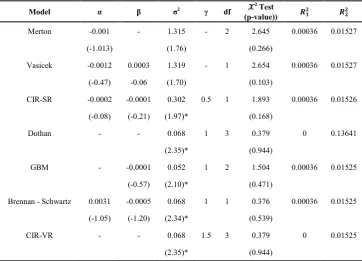
Table 3. Regression results for full sample observation
Model α β σ2 γ df 𝒳𝒳2 Test
(p-value)) 𝑹𝑹𝟏𝟏𝟐𝟐 𝑹𝑹𝟐𝟐𝟐𝟐
Merton -0.001 - 1.315 - 2 2.645 0.00036 0.01527
(-1.013) (1.76) (0.266)
Vasicek -0.0012 0.0003 1.319 - 1 2.654 0.00036 0.01527 (-0.47) -0.06 (1.70) (0.103)
CIR-SR -0.0002 -0.0001 0.302 0.5 1 1.893 0.00036 0.01526 (-0.08) (-0.21) (1.97)* (0.168)
Dothan - - 0.068 1 3 0.379 0 0.13641
(2.35)* (0.944)
GBM - -0.0001 0.052 1 2 1.504 0.00036 0.01525 (-0.57) (2.10)* (0.471)
Brennan - Schwartz 0.0031 -0.0005 0.068 1 1 0.376 0.00036 0.01525 (-1.05) (-1.20) (2.34)* (0.539)
CIR-VR - - 0.068 1.5 3 0.379 0 0.01525
(2.35)* (0.944)
As shown in Table 3, the models vary in their explanation power for interest rate changes. The 𝑅𝑅12 of the short rate models are mostly below 0.01% and slightly different from one to the others. The 𝑅𝑅22, however, show higher value ranging from 0.015 (GBM [6], Brennan-Schwartz [8], and CIR-VR [11] ) to 0.13 (Dothan [14] ). This result also shows that the 𝑅𝑅12 for Dothan [14] and CIR-VR [11] level equation is zero because the parameter α and β for both models is restricted to zero. Thus, the level equation cannot be estimated. In addition to that, the volatility equations have larger 𝑅𝑅22 than level equations. Based on 𝑅𝑅22 result, the best volatility model is Merton [1]. In table 3, the χ2 tests for goodness-of-fit also suggest that all models are correctly specified. Those short rate models have χ2 values below 6 and therefore, it can not be rejected at 95% confidence level. This result is different from the results in CKLS [10], in which the models with low γ values are misspecified.
The rt, the annualized one-month United Kingdom interbank rate, is estimated using data from January 1975 to July 2010 (9281 daily data). The parameters are obtained by performing regression using system of Generalized Method of Moments. Moreover, the 𝑅𝑅𝑗𝑗2 statistics are computed as
the proportion of total variation of actual rate changes (j=1) and the volatility (j=2) explained by the respective predictive value for every model. The 𝒳𝒳2 statistics are reported with associated degree of freedom (df) and its p-value in parentheses.
Table 4 displays the comparison result between restricted models and less restricted model by using Wald coefficient test [24]. Low probability in the Wald test indicates that the null hypothesis of restricted parameter is strongly rejected. Thus, the result in Table 4 shows that the more restricted model is not preferable than the less restricted one (i.e. Merton [29] cannot be rejected against the alternative of Vasicek [41], Dothan [14] cannot be rejected against GBM [6], GBM [6] and Dothan [14] cannot be rejected against Brennan - Schwartz [8]).
[image:5.595.314.554.152.279.2]The parameter restriction is performed using Wald test
Table 4. Pairwise comparison of short rate models
Alternative
Model Restricted Model 𝓧𝓧𝟐𝟐Statistic Probability
Vasicek Merton 0.004 0.95
GBM Dothan 0.325 0.569
Brennan -
Schwartz Dothan 1.453 0.484 Brennan -
Schwartz GBM 1.119 0.29
Furthermore, this paper investigates the impact of structural break to the performance of short rate models. The structural break is specified at 16 September 1992 when UK withdrew pound sterling from European exchange rate mechanism. The policy resulted in a drastic increase of 1-month UK interbank rate from 10.3 % in 15 September 1992 to 20.5% in 16 September 1992. Following that event, Central Bank of United Kingdom adopted and instituted its
inflation targeting regime starting October 1992.
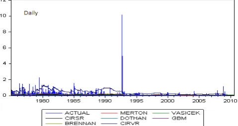
Figure 2 compares the forecasted volatility versus the actual volatility of all short rate models using short rate data for all sample period (1975 to 2010). It is apparent that the interest rate change prior to Black Wednesday is less volatile than the changes after Black Wednesday.
Figure 2. Actual vs forecast volatility for full sample observation (1975-2010)
[image:5.595.321.541.466.652.2]Table 5 shows the result of Chow test which measure the importance of structural break. To perform Chow test, sample data is divided into two parts, before and after 16 September 1992 (Black Wednesday). Then, the regression is estimated for both sub-period and compared using F-test. The result shows that there are mixed evidences regarding the significance structural break. For instance, table 5 shows that for the level equation (equation (2)), most of the models rejected structural break except Vasicek [41] and CIR-SR [12] models. For variance equation (equation (3)), however, Merton [29], Vasicek [41], CIR-SR [12 ] and Dothan [14] supported structural breaks.
Table 5. Chow Test
Model F-statistic
Level Equation Variance Equation
Merton 0.88 3.34*
Vasicek 3.43* 4.98**
CIR-SR 3.14* 2.91*
Dothan 18411**
GBM 1.77 -0.08
Brennan 1.49 0.58
CIR-VR -1.23
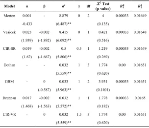
[image:5.595.58.298.556.649.2]Table 6. Regression Results using data before Black Wednesday
Model α β σ2 γ df 𝒳𝒳2 Test
(p-value) 𝑹𝑹𝟏𝟏𝟐𝟐 𝑹𝑹𝟐𝟐𝟐𝟐
Merton 0.001 - 8.879 0 2 4 0.00033 0.01649 -0.433 (6.487)** (0.135)
Vasicek 0.023 -0.002 8.415 0 1 0.421 0.00033 0.01648 (1.939) (-1.892) (6.092)** (0.516)
CIR-SR 0.019 -0.002 0.5 0.5 1 1.219 0.00033 0.01649 (1.62) (-1.667) (5.806)** (0.269)
Dothan - - 0.032 1 3 1.774 0.00 0.01651 (5.559)** (0.620)
GBM - 0 0.033 1 2 3.931 0.00033 0.01651 (-0.587) (5.963)** (0.1401)
Brennan 0.017 -0.002 0.032 1 1 1.778 0.00033 0.0165 (1.468) (-1.563) (5.572)** (0.182)
CIR-VR - 0 0.032 1.5 3 1.774 0.00 0.01651 (5.559)** (0.620)
Notes: **, indicates significance at 5 percent levels, respectively
The estimation horizon for rt, the annualized one-month United Kingdom interbank rate started from January 1975 to September 1992 (4619 observations). The parameters are estimated using system of Generalized Method of Moments with t-statistics in parentheses.
Table 6 shows that none of parameter α and β is significantly different from zero in each model, but parameter σ2 is highly significant at 1% level for all models. In addition to that, the best variance model based on 𝑅𝑅22 is GBM [6] and Dothan [14].
Table 7. Regression Results using data after Black Wednesday
Model α β σ2 γ df 𝒳𝒳2 Test
(p-value) 𝑹𝑹𝟏𝟏𝟐𝟐 𝑹𝑹𝟐𝟐𝟐𝟐
Merton -0.001 - 0.81 0 2 1.091 0.0005 0.00904 (-1.774) (4.029)** (0.579)
Vasicek -0.002 0.00002 0.844 0 1 1.422 0.0005 0.00904 (0.140) (0.0072) (4.494)** (0.233)
CIR-SR -0.001 -0.0001 0.178 0.5 1 1.366 0.0005 0.00902 (-0.111) (-0.044) (2.247)* (0.242)
Dothan - - 0.033 1 3 1.091 0.000 0.00902 (1.708) (0.779)
GBM - -0.0004 0.033 1 2 1.142 0.0005 0.00897 (-1.679) (1.748) (0.564)
Brennan -0.002 -0.00001 0.033 1 1 1.371 0.0005 0.00901 (-0.160) (-0.005) (1.896) (0.241)
CIR-VR - - 0.033 1.5 3 1.091 0.000 0.00902 (1.708) (0.779)
Notes: *, ** indicates significance at 5 percent, and 1 percent levels, respectively
[image:6.595.152.457.88.350.2] [image:6.595.154.456.448.702.2]Table 7 shows that among all the parameters in short rate models (α, β, and σ2), only parameter σ2 is significant at 1% (i.e. Merton [29] and Vasicek [41] models). Moreover, σ2 is significant at 5% for the CIR-SR [12]. The best volatility equation based on 𝑅𝑅22 is Vasicek [41].
Both full sample and separate sample data provide different results with those of CKLS [10] in which models that with γ ≤ 1 capture short term interest rates dynamics better than those with γ ≥ 1. Following the results of Mahdavi [28], this study also show that no single model can explain short rate diffusion for all countries and data sets. The result in CKLS [10] may hold for one-month U.S. Treasury bill yield, but does not hold for one-month UK interbank rate. Moreover, the result in this study demonstrates that single factor short rate model results are sensitive to selection of structural break point in the data set. In most cases, however, volatility remains an important feature in explaining the dynamics of short rate.
5. Conclusions
The article attempts to examine the performance of various different single factor models to explain UK short rate dynamics. Controlling for structural break in the data set, this study finds mixed conclusion for the best single factor short rate model. Additionally, the result of pairwise comparison between restricted and unrestricted models shows that the more restricted model is not rejected against the less restricted one. Moreover, similar to Bliss and Smith [7], the result of this study contradicts the main result of CKLS [10]. This study shows that models which allow the volatility of interest rate changes to be highly sensitive to the level of riskless rate are not necessarily more successful in capturing the dynamics of short rate. This study, however, support CKLS [10] conclusion that volatility equation is the most important part of single factor short rate predictive models. This result is consistent using full sample or separate sample observations.
The results of this study have important implication for the improvement of current single factor short rate models. This study documents that single factor short rate model remains a valuable tool to describe the spot rate movement. Although GARCH, regime-switching, and jumps features are essential for modelling certain spot rate dynamics, their specification may not be suitable to model spot rate dynamics in a country where short rate are subject to extensive government control (Hong [20]). Furthermore, by comparing various single factor diffusion functions with linear drift, this study has also shown that although volatility is an important part of single factor short rate models, the sensitivity of volatility does not always proportionally affect the performance of single factor short rate models. Finally, future studies in this area should consider using variety of econometric technique including efficient method of moments and nonparametric estimators.
Acknowledgements
I am very grateful for the comments and suggestions from all participants at IV World Finance Conference 2013.
REFERENCES
[1] Aït Sahalia, Y. (1996) Testing continuous-time models of the spot interest rates, Review of Finance Studies, 9, 385–426. [2] Andersen, T.G., Lund, J. (1997) Estimating continuous-time
stochastic volatility models of the short-term interest rate, Journal of Econometrics, 77, 343–377.
[3] Ang, A., Bekaert, G. (2002) Regime switches in interest rates, Journal of Business and Economic Statistics, 20, 163–182. [4] Bali, G., Wu, L. (2006) A comprehensive analysis of the
short-term interest rate dynamics, Journal of Banking and Finance, 30, 1269-1290.
[5] Benati, L. (2006) UK monetary regimes and macroeconomic stylised facts. Working Paper no. 290, Bank of England. [6] Black, F. and Scholes M. (1973) The pricing of options and
corporate liabilities, Journal of Political Economy, 81, 637-654.
[7] Bliss, R. R. and Smith, D. C. (1998) The Elasticity of Interest Rate Volatility: Chan, Karolyi, Longstaff, and Sanders Revisited, Journal of Risk, 1, no. 1 (Fall): 21-46.
[8] Brennan, M. J. and Schwartz, E. S. (1980) Analyzing convertible bonds, Journal of Financial and Quantitative Analysis, 15, 907-929.
[9] Brenner, R. J., Harjes, R. H. and Kroner, K. F. (1996) Another look at models of the short-term interest rate, Journal of Financial and Quantitative Analysis, 31, 85-107.
[10] Chan, K., Karolyi, A., Longstaff, F., and Sanders, A. (1992) An Empirical comparison of alternative models of the short-term interest rate, Journal of Finance, 47, 1209-1227. [11] Cox, John, C. Jonathan E. I., and Stephen A. R. (1980) An
analysis of variable rate loan contracts, Journal of Finance,35, 389-403.
[12] Cox, John, Jonathan E. I. and Stephen A. R. (1985) A theory of the term structure of interest rates, Econometrica, 53, 385-407.
[13] Dahlquist, M. (1996) On alternative interest rate processes, Journal of Banking and Finance, 20, 1093-1119.
[14] Dothan, U. L. (1978) On the term structure of interest rates, Journal of Financial Economics, 6, 59-69.
[15] Duffie, D., & Kan, R. (1996) A yield-factor model of interest rates, Mathematical Finance, 6, 379−406.
[16] Gibbons, M. R. and Ramaswamy, K. (1986) The term structure of interest rates: empirical evidence, Working paper, Stanford University.
Financial Economics, 42, 27-62.
[18] Hansen, L. P. (1982) Large sample properties of Generalized Method of Moments Estimators, Econometrica, 50, 1029-1054.
[19] Harvey, C.(1988) The real term structure and consumption growth, Journal of Financial Economics, 22, 305-333. [20] Hong, Y., Li, H. (2005) Nonparametric specification testing
for continuous-time models with applications to term structure of interest rates, Review of Financial Studies, 18, 37–84.
[21] Hong, Y., Lin, H., and Wang, S. (2010) Modeling the dynamics of Chinese spot interest rates, Journal of Banking and Finance, 34, 1047-1061.
[22] Hull, J. and White, A. (1990) Pricing interest-rate derivative securities, Review of Financial Studies, 3, 573-592.
[23] Jiang, G., Yan, S. (2008) Linear-quadratic term structure models: Toward the understanding of jumps in interest rates, Journal of Banking and Finance, 33, 473–485.
[24] Kan, R. and Zhang,C. (1999) GMM Tests of stochastic discount factor models with useless factors, Journal of Financial Economics, 54, 103-127.
[25] Leippold, M., & Wu, L. (2002) Asset pricing under the quadratic class, Journal of Financial and Quantitative Analysis, 37, 271−295.
[26] Longstaff, F. A. and Schwartz, E. S. (1992) Interest-rate volatility and the term structure: A two-factor general equilibrium model, Journal of Finance, 47, 1259-1282. [27] Longstaff, F. A. (1989) A nonlinear general equilibrium
model of the term structure of interest rates, Journal of Financial Economics, 23, 195-224.
[28] Mahdavi, M. (2008) A comparison of international short-term rates under no arbitrage condition, Global Finance Journal, 18, 303-318.
[29] Merton, R. C. (1973) An intertemporal capital asset pricing model, Econometrica,41, 867–87.
[30] Newey, W. and West, K. (1987) Hypothesis testing with efficient method of moments estimation, International Economic Review, 28, 777-787.
[31] Nowman, B. K. and Sorwar, G. (1999) An evaluation of contingent claims using the CKLS interest rate model: an analysis of Australia, Japan and United Kingdom, Asia-Pacific Financial Markets, 6, 205-219.
[32] Nowman, B. K. (1997) Gaussian estimation of single-factor continuous time models of the term structure of interest rates, Journal of Finance, 52, 1695-1706.
[33] Pritsker, M. (1998) Nonparametric density estimation and tests of continuous time interest rate models, Review of Financial Studies, 11, 449–487.
[34] Sam, A. and Jiang, G. (2009) Nonparametric Estimation of the Short Rate Diffusion Process from a Panel of Yields, The Journal of Financial and Quantitative Analysis, 44, 1197-1230.
[35] Sanders, A. B. and Unal, H. (1988) On the intertemporal behavior of the short-term rate of interest, Journal of Financial and Quantitative Analysis, 23, 417-423.
[36] Sorwar, G. (2011) Estimating single factor jump diffusion interest rate models, Applied Financial Economics, 21. [37] Sorwar, G., Barone-Adesi, G., Allegretto, W. (2007)
Valuation of derivatives based on single-factor interest rate models, Global Finance journal, 18, 251-269.
[38] Stanton, R. (1997) A nonparametric model of term structure dynamics and the market price of interest rate risk, Journal of Finance, 52, 1973–2002.
[39] Treepongkaruna, S., & Gray, S. (2003). On the robustness of short–term interest rate models, Accounting & Finance, 43(1), 87-121.
[40] Tse, Y. K. (1995) Some international evidence of stochastic behaviour of interest rates, Journal of International Money and Finance, 14, 721-738.