Time trend in spatial dependence: Specification strategy in the first order spatial autoregressive model

Munich Personal RePEc Archive

Time-trend in spatial dependence:

Specification strategy in the first-order

spatial autoregressive model

López, Fernando and Chasco, Coro

Universidad Autónoma de Madrid

3 March 2007

Online at

https://mpra.ub.uni-muenchen.de/1985/

TIME-TREND IN SPATIAL DEPENDENCE: SPECIFICATION STRATEGY IN

THE FIRST-ORDER SPATIAL AUTOREGRESSIVE MODEL

Fernando A. López-Hernández

Departamento de Métodos Cuantitativos e Informáticos Universidad Politécnica de Cartagena

30203 Cartagena (Spain) Email: [email protected]

Coro Chasco-Yrigoyen

Departamento de Economía Aplicada Universidad Autónoma de Madrid 28049 Madrid (Spain)

Email: [email protected]

Abstract. The purpose of this article is to analyze if spatial dependence is a synchronic effect in the first-order spatial autoregressive model, SAR(1). Spatial dependence can be not only contemporary

but also time-lagged in many socio-economic phenomena. In this paper, we use three Moran-based

space-time autocorrelation statistics to evaluate the simultaneity of this spatial effect. A simulation

study shed some light upon these issues, demonstrating the capacity of these tests to identify the

structure (only instant, only time-lagged or both instant and time-lagged) of spatial dependence in

most cases.

Key words: Space-time dependence, Spatial autoregressive models, Moran’s I.

Resumen. En este artículo, se analiza la instantaneidad de la dependencia especial en el modelo auto-regresivo espacial de primer orden o SAR(1). En muchos fenómenos socioeconómicos, el

fenómeno de dependencia especial puede ser no sólo contemporáneo o instantáneo, sino también

retardado en el tiempo. Con ayuda de tres estadísticos espacio-temporales basados en el test I de

Moran, evaluaremos la instantaneidad de este efecto especial. Además, se demostrará la

capacidad de dichos tests para identificar la estructura de dependencia espacial (sólo instantánea,

sólo retardada en el tiempo y mixta) de la mayoría de las distribuciones, a través de un ejercicio de

simulación de Monte-Carlo.

Key words: Dependencia espacio-temporal, Modelos espaciales auto-regresivos, I de Moran.

1 INTRODUCTION

The purpose of this article is to analyze the time-trend of spatial dependence in the first-order

spatial autoregressive model, SAR(1), making a differentiation between two types of spatial

dependence: contemporary or instant and non-contemporary or time-lagged. The first type is the

consequence of a very quick interaction of the process over the neighboring locations, while the

second implies that a shock in a certain location needs some time to extend over its neighborhood.

It is not easy to separate both types of spatial dependence but both are present very frequently and

should be considered when specifying a spatial autoregressive model.

Spatial dependence has usually been defined as a spatial effect, which is related to the

spatial interaction existing between geographic locations and takes place in a particular moment of

time. In other words, spatial dependence is considered as the contemporary coincidence of value

similarity with locational similarity. When spatial interaction, spatial spillovers or spatial hierarchies

produce spatial dependence in the endogenous variable of a regression model, the spatial

autoregressive model has been frequently mentioned as the solution in the literature (e.g. Florax et

al. 2003). Analogous to the Box-Jenkings approach in the time-series analysis, spatial model

specifications consider autoregressive processes. Particularly, in the first-order spatial

autoregressive model, SAR(1), a variableis a function of its spatial lag(a weighted average of the

value of this variablein the neighboring locations) for a same moment of time.

However, in most socio-economic phenomena, this coincidence in values-locations is not

only an instant coincidence but also (or perhaps only) a final effect of some cause that happened in

the past, one that has spread through geographic space during a certain period. In this sense, there

are some authors that have considered this pure simultaneity of spatial dependence as problematic

(Upton and Fingleton 1985, pp 369), suggesting the introduction of a time-lagged spatial

dependence term. Moreover, Cressie (1993, pp 450) proposes a generalization of the STARIMA

models presented in Martin and Oeppen (1975) and Pfeifer and Deutsch (1980), among others,

such that they also include not only time-lagged but also “instantaneous spatial dependence”.

Recently, there are several contributions in this subject. For example, Elhorst (2001, 2003)

presented several single equation models that include a wide range of substantive

non-contemporary spatial dependence lags, not only in the endogenous but also in the exogenous

variables. Anselin et al. (2005) present a brief taxonomy for panel data models with different kind of

spatial dependence structure for the endogenous variable (space, time and space-time), referring to

them as pure space-recursive, time-space recursive, time-space simultaneous and time-space

Space-time dependence has also been specified in spatial autoregressive models in either

theoretical frameworks (Baltagi et al. 2003; Pace et al. 1998, 2000) or panel data applications

(Case 1991; Yilmaz et al. 2002; Baltagi and Li 2003; Mobley 2003).

In this article, we analyze if spatial dependence is a synchronic effect in the SAR(1) model,

allowing for not only horizontal (static) but also space-time interaction (dynamic). Similarly as in

Pace et al. (1998, 2000), it is our aim to identify different components in the spatial lag term,

splitting it into instant, space-time or both –instant and space-time- spatial dependence

components. Therefore, we propose the identification and use –if necessary- of the space-time

lagged endogenous variable in the SAR(1) model, since it reflects the effects due to spatial

interaction as a spatial diffusion phenomena, which is not only “horizontal” – simultaneous – but

also time-wise.

For this purpose, we present some space-time Moran-based statistics in order to identify the

spatial dependence structure in the SAR(1) model. We illustrate the performance of these statistics

with a simulation exercise.

The remainder of paper is organized as follows. In the next section, we derive three

Moran-based autocorrelation statistics to evaluate the simultaneity of the SAR(1) model. In section 3, we

present three different specifications of spatial dependence in this model, as well as the behavior of

the identification statistics in each one. In section 4, we evaluate the power of the tests with a

simulation analysis. Some summary conclusions and references complete the paper.

2 MORAN SPACE-TIME STATISTICS FOR THE EVALUATION OF SPATIAL DEPENDENCE IN THE FIRST-ORDER SPATIAL AUTOREGRESSIVE MODEL

The first-order spatial autoregressive model, SAR(1), or simultaneous model dates back to the work

of Whittle (1954). In matrix notation, it takes the form:

(

2

)

0,

_n

z

Wz

N

I

ρ

ε

ε

σ

=

+

∼

(1)

where

z

=

[

y

−

y

] /

σ

_y is a n by 1 vector of observations (variable vector y is expressed in

deviations from the means form to eliminate the constant term in the model); W is the spatial weight

is the familiar spatial weight matrix that defines the neighborhood interactions existent in a spatial

sample (Cliff and Ord 1981). In this context, the usual row-standardized form of the spatial weights

matrix can be used, yielding an interpretation of the spatial lag (Wz) as an “average” of neighboring

values.

The spatial term, Wz, is a way to assess the degree of spatial dependence of zin a same

moment of time (from now on, it is denoted as Wzt). Nevertheless, in most socio-economic

phenomena, the relationship between zt and Wzt is not only synchronic but also –or perhaps only- a

final effect of some cause that happened in the past (Wzt-k;

k

=

1, 2,...

). Consequently, before

estimating a SAR(1) model, we should identify correctly the form of the spatial effect, Wzt, in this

model.

In this section, we present some Moran-based statistics that are useful to detect the

existence of time-lagged spatial dependence. First, we briefly present the space-time Moran’s I

statistic (STI), which evaluates spatial dependence in two instant of time. Secondly, we present two

partial space-time Moran’s functions: the partial time-lagged Moran’s I (PLI) and the partial instant

Moran’s I (PII). Our goal is to contribute towards obtaining appropriate indicators to evaluate the

temporal structure of spatial dependence in the SAR(1) model.

2.1 Space-time autocorrelation

When considering both space-time dimensions, some Moran-based statistics can be defined

to analyze and visualize the space-time structure of a distribution (Anselin et al. 2002). This is the

case of the space-time Moran’s I (STI). This instrument is similar to others already proposed in the literature (e.g. Cliff and Ord 1981, pp. 23).

The STI is an extension of Moran’s I. It computes the relationship between the spatial lag,

Wzt, at time t and the original variable, z, at time

t

−

k

(k is the order of the time lag). Therefore,

this statistic quantifies the influence that a change in a spatial variable z, that operated in the past

(

t

−

k

) in an individual location i (zt-k) exerts over its neighborhood at present (Wzt). Hence, it is

possible to define it as follows:

,

t k t t k t

t k t k

z Wz

I

z

z

− −

− −

′

=

where, the denominator can be substituted by n as this variable z is also standardized. The value

adopted by this index, corresponds with the slope in the regression line of Wzton zt-k. Note that for

0

k

=

, this statistic coincides with the familiar univariate Moran’s I that from now on, we denote as

It.

The significance of this statistic can be assessed in the usual fashion by means of a

randomization (or permutation) approach. In this case, the observed values for one of the variables

are randomly reallocated to locations and the statistic is recomputed for each such random pattern.

A space-time Moran’s I function could be considered. It is the result of plotting all the values

of the STI statistic, adopted by a variable z in time t, for different time lags k. The first value

corresponds to the contemporary case, k=0, which is the univariate Moran’s I (It), whereas the other ones are proper space-time Moran’s I coefficients (It-k,t). This function is a particular case of

the “full” space-time autocorrelation function (Pfeifer and Deutsch 1980, Bennett 1979), which is a

3-D plot that includes the correlation coefficients for all the space and time lags of a distribution.

2.2 Moran space-time partial autocorrelation statistics

There is no doubt that the spatial dependence measures that have been presented include

different sources of dependence that are difficult to separate.

(

_it

,

_js

)

0

Cov z z

≠

(3)

where sub-indexes i, j are different spatial locations and t, s are different instants of time.

Therefore, we consider the following types of dependencies:

(a) There is a dependence in expression (4) that is the result of time evolution:

(

_it

,

_js

)

0

Cov z z

≠

;

∀ =

i

j

(4)

This expression affirms that (for

s

= −

t

k

) the value of the z variable in period t is more or

less related to

t

−

k

. This assertion is more correct for lower values of k.

(

_it

,

_js

)

0

Cov z z

≠

;

∀ =

t

s

(5)

This second type of dependence –spatial dependence- can be produced by two sources:

(b1) Simultaneous or contemporary spatial dependence constitutes the usual definition of spatial dependence in the literature and it is the consequence of an instant, very rapid, spatial

diffusion of a phenomenon in geographic space. It can be connected to or the consequence of a

lack of concordance between a spatial observation and the region in which the phenomenon is

analyzed.

(b2) Time-lagged or non-contemporary spatial dependence is the result of a slower diffusion of a phenomenon towards the surrounding space. This kind of dependence is due to the usual

interchange flows existing between neighboring areas, which requires of a certain time to be tested.

Although it is very difficult to divide spatial dependence into its two dimensions (instant and

time-lagged), it is worth trying to compute them separately in order to correctly specify a spatial

process that exhibits spatial dependence. One of the aims of this article is to show a new range of

Moran-based statistics that allow justifying the inclusion of both kind of spatial lags, contemporary

(Wzt) and time-lagged (Wzt-k) ones, to explain ztin a spatial regression. Some coefficients can be

defined to evaluate the inclusion of a space-time lag term in a spatial regression.

Since the space-time Moran’s I (STI) –equation (2)- equals to the slope of the regression of

Wzt-k on zt, it is possible to connect this statistic with the standard Pearson correlation coefficient

between these two variables, as also derived by Lee (2001). So we can express the STI statistic as:

, t k, t

(

)

t k t z Wz t

I

₋

=

r

₋

Var Wz

(6)

where _,

t t k z Wz

r

₋ is the Pearson linear correlation coefficient between zt-kand Wzt.

The basic underlying idea consists of eliminating the influence of one of the dimensions in

order to compute separately contemporary and non-contemporary spatial dependence. For this

purpose, we substitute in (6) the space-time correlation coefficient by a partial correlation one. Two

(a) Partial Time-Lagged Moran’s I (PLI) computes the correlation between variable z in period t-k

and its spatial lag Wz in period t removing the influence of z in t:

,

(

,

)

(

)

;

1, 2,...,

1

P

t k t t k t t t

I

₋

=

Corr z

₋

Wz z

Var Wz

k

=

t

−

(7)

where , , ,

2 2

, ,

(

,

)

1

1

t k t t

t

t t k t t t k

t t t

t k

z z

z Wz Wz z

z z Wz z

Corr z

Wz z

r

r

r

r

r

− − − −

⋅

=

⋅

−

−

−

is the partial correlation coefficient of

variables zt-k and Wzt after eliminating the correlation from zt. Therefore, it is possible to express this

statistic as a function of both Moran’s I and space-time Moran’s I:

,

,

, _{2 2}

, ,

1

1

t t k

t k t t P

t k t

z z z Wz t t k

t t

z z

I

I

r

r

I

r

− − − − ⋅

−

⋅

=

−

−

(8)

This indicator removes contemporary spatial dependence from the relationship between

variables zt-k and Wzt. If the pattern of spatial dependence is one that can be totally captured by

contemporary spatial dependence (

I

_t

≠

0

), then the PLI will be close to zero. On the contrary, if

the process is one that can be captured by non-contemporary spatial dependence, then

I

_{t k t}P_{− ,} will

be significantly different from zero. Regarding to the sign, it is positive/negative depending on It-k,t

sign.

(b) Partial Instant Moran’s I (PII) is the complementary expression that consists of computing contemporary –or instant- spatial dependence after removing time-lagged spatial dependence

by means of an index:

( ,

)

(

)

;

1, 2,...,

1

k

P

t t t t k t

I

=

Corr z Wz z

₋

Var Wz

k

=

t

−

(9)

where

Corr z Wz z

( ,

_{t t t k−}

)

is the partial correlation coefficient of variables zt and Wzt after

eliminating the correlation from Wzt-k. Therefore, it is possible to express this statistic as a function

, 2 2 , , ,

1

1

k t t

t k t k

t t k t P

t

z z Wz z t t k z z

I

I

r

r

r

I

− − − − ⋅

−

⋅

=

−

−

(10)

This indicator removes time-lagged spatial dependence from the contemporary spatial

relationship between variables zt and Wzt. If the pattern of spatial dependence is one that can be

totally captured by a time-lagged spatial autoregression, then the PPI will be close to zero. On the

contrary, if the process is one that can be captured by contemporary spatial dependence, then PPI

will be significantly different from zero.

From (8) and (10), it is easy to derive the following expression:

-- -2 2 , , , - , 2 2 , ,

1-

1-

·

;

1, ..., -1

1-

1-t t t k t t t k _k

t t

t k t k

Wz z P Wz z z z P

t t t k t

z z z z

r

r

r

I

I

I

k

t

r

r

=

+

=

(11)

In this expression, spatial dependence (measured with Moran’s I statistic or

I

_t) is shown as

the sum of two contributions: contemporary spatial dependence (PII or Pk

t

I

) and non-contemporary

spatial dependence (PLI or

I

_{t k t}P_{- ,} ), both weighted by a corresponding scalar.

In case of normal distribution, the inference of the common partial correlation coefficient can

be applied to both Moran space-time partial autocorrelation statistics, as they are the result of

multiplying the former by a constant. In case of non-normality, a permutation approach can be the

solution to compute the moments.

3. IDENTIFICATION OF SPATIAL DEPENDENCE STRUCTURE IN THE FIRST-ORDER SPATIAL AUTOREGRESSIVE MODEL

The joint representation of the space-time Moran’s I coefficient (STI) in combination with the Moran

space-time partial autocorrelation statistics (PLI, PII) is a useful tool to identify the simultaneity of

spatial dependence in the SAR(1) model. The identification of spatial dependence structure should

be conducted in two steps as follows:

the regular inference process), we can conclude that there is time-lagged spatial dependence in the

corresponding distribution, and vice versa.

Step 2. Secondly, the Moran space-time partial autocorrelation statistics (PLI, PII) are the instrument to determine whether the existent spatial dependence contains an instant and/or

time-lagged component.

Contemporary or instant spatial dependence is present in a variable if only the partial instant Moran’s I (PII) has significant values. In this case, only the present values of the variable(zt)

can explain its present spatial lag (Wzt). In a spatial regression, if an endogenous variable zt

exhibits significant STI and PII values, we could capture spatial autocorrelation by a contemporary

spatial lag of zt(Wzt) as an explicative variable in the model.

t t t

z

=

ρ

Wz

+

ε

(12)

where ρ is the spatial parameter to estimate and ε the error term. This is the SAR(1) model.

Non-contemporary or time-lagged spatial dependence is present in a variable if only the partial time-lagged Moran’s I (PLI) has significant values. In fact, past values of variable z (zt-k)

completely explain its present spatial lag (Wzt). In this case, we could capture spatial dependence

in an endogenous variable zt introduction a space-time lag of z (Wzt-k) as an explicative, exogenous,

variable in the model.

t t k t

z

=

ρ

Wz

₋

+

ε

(13)

Mixed contemporary and non-contemporary spatial dependence is present in a variable if both partial functions have high significant values for the same periods. In this case, not only

present but also past values of variable z can completely explain its present spatial lag. Therefore,

we could capture spatial dependence in an endogenous variable zt specifying both an instant and a

time-lagged spatial lag of z (Wzt, Wzt-k) as explicative variables in the model.

t 1 t 2 t k t

where ρ1, ρ2 are spatial parameters to estimate. This model is the mixed regressive-spatial autoregressive model or space lag model, which includes as explicative not only the spatial-lagged

endogenous variable (Wzt), but also real exogenous variables (Wzt-k).

4. MONTE CARLO SIMULATION STUDY

Next, we evaluate empirically the Moran space-time autocorrelation statistics (STI, PLI, PII) in a

series of Monte Carlo simulation in order to obtain an initial assessment of their discriminating

power of spatial dependence into instant and/or time-lagged.

5.1. Experimental design

We consider two different moments of time t, s, such that

s

<

t

. For time s, we generate an

instant spatial dependence process (zs) whereas for time t we set up three alternative processes

(zt): instant spatial dependence (i), time-lagged spatial dependence (ii) and both instant and

time-lagged spatial dependence (iii). Formally:

i) For time t, instant spatial dependence only:

s s s

t t t

z

Wz

z

Wz

ρ

ε

ρ

ε

=

+

=

+

(15)

ii) For time t, time-lagged spatial dependence only:

=

+

=

+

s s s

t s t

z

Wz

z

Wz

ρ

ε

ρ

ε

(16)

iii) For time t, both instant and time-lagged spatial dependence:

1 2

s s s

t t s t

z

Wz

z

Wz

Wz

ρ

ε

ρ

ρ

ε

=

+

=

+

+

(17)

where ρ, ρ1, ρ2 are the spatial autoregressive coefficients and εs, εt are the error terms for time s, t, respectively. For the sake of simplicity, we specify the same spatial weight matrix, W, in all cases. It

Clearly, we can obtain different degrees of instant and time-lagged spatial dependence by

manipulating the values of the parameters and the characteristics of the error terms. In our

experiments, we set the purely temporal dependence structure in variable z by means of the error

terms (εs, εt), which are generated as a bivariate normal distribution with zero mean and

Σ =

( )

σ

ij

covariance matrix, such that

σ

_ii

=

1

and

σ

_ij

=

r

. Temporal autocorrelation is defined by the r

parameter considering three different cases: weak temporal autocorrelation (

r

=

0.5

), moderate temporal autocorrelation (

r

=

0.75

) and strong temporal autocorrelation (

r

=

0.98

).

The spatial configuration we have consider is a regular lattice structure for a queen-type

contiguity in square 10 by 10 (N = 100). The spatial weights matrix is used in row-standardized

form.

In the case of expression (17) –both instant and time-lagged spatial dependence in time t,

we also consider two different intensities in spatial dependence:

a) Stronger instant spatial dependence:

ρ

₁

=

2

ρ

₂

and

ρ ρ

₁

+

₂

=

ρ

b) Stronger time-lagged spatial dependence:

2

ρ

₁

=

ρ

₂

and

ρ ρ

₁

+

₂

=

ρ

Therefore, we compute the space-time partial autocorrelation statistics in time t, with

respect to time s, for the different values of parameters r, ρ. We have only considered positive spatial autocorrelation structures, which is the most common tendency found in empirical cases

(Griffith and Arbia 2006). In the simulations, we let ρ vary from 0 to 1, with increments of 0.05, to assess the effect of spatial lag autocorrelation. We have generated 9,999 replications for each

situation. We have evaluated the power of the test statistics (STI, PLI, PII) to discriminate between

instant, time-lagged or both kind of spatial dependence structure in the SAR(1) model.

5.2. Power of the tests

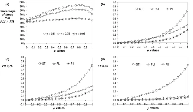
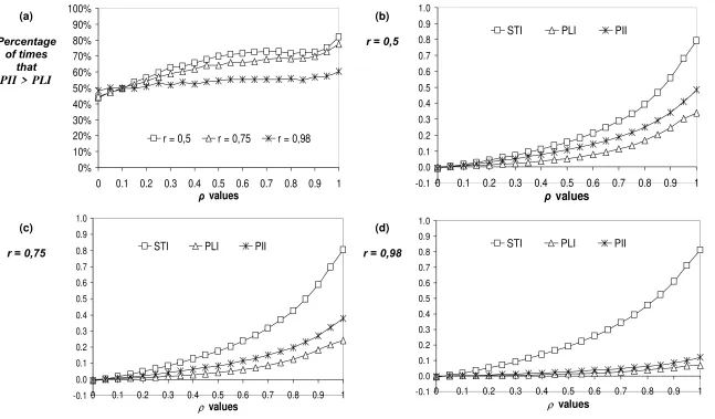
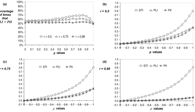
Figures 1-4 present the simulation results. In the upper-left cell, we have plotted the power

of the selection criterion as the number of times that a partial index is higher than the other one.

The rest of the graphs show the average values of the STI, PLI and PII for the three types of

temporal autocorrelation (

r

=

0.5, 0.75, 0.98

). Each Figure specifies a different data generating

In Figure 1, which corresponds to model (15), the average values of PII are quite similar to

STI ones, while PLI adopts almost zero values. This gap is higher for lower temporal autocorrelation

(

r

=

0.5, 0.75

), but in the case of

r

=

0.98

, though PLI values are almost zero, PII coefficients

move down away from STI. It is a natural effect, since such a strong temporal autocorrelation

(

r

=

0.98

) induces an even stronger correlation between zt and zs (0.998) what leads to a practical identification between both processes. Regarding the power of the partial tests (number of times

PII

>

PLI

) to select the correct model, it loose strength with higher temporal correlation (r), but it augments with stronger spatial autocorrelation (ρ).

When having the pure time-lagged spatial dependence situation shown in (16), both partial

tests get positive average values (Figure 2). These figures decline with temporal autocorrelation so

that in the extreme case of

r

=

0.98

, both PII and PLI are nearly zero. In this situation, the number of times

PLI

>

PII

is around 80% for moderate time-lagged spatial dependence (

ρ

≥

0.4

) and

weak temporal correlation (

r

=

0.5

). This percentage declines for higher levels of temporal correlation but increases with spatial autocorrelation.

The situation described in model (17) –mixed instant and time-lagged spatial dependence-

is more difficult to detect because they are intermediate cases between models (15) and (16). As

previously described, we have considered two states: stronger instant spatial dependence (Figure

3) and stronger time-lagged spatial dependence (Figure 4). In the first case, PII is always over PLI,

though the gap is not as steeper as in the generating process shown in Figure 1. That is why the

percentage of times that PII>PLI is smaller (about 70%). As in the other cases, higher temporal

correlation produces an identification of both processes zt and zs, so that it is more difficult to

differentiate between them.

5 CONCLUSIONS

The main aim of this paper is to analyze to what extent spatial dependence is an instantaneous

effect in the SAR(1) model, making a differentiation between instant or contemporaneous and

lagged or non-contemporaneous spatial dependence. The first is the consequence of a very quick

diffusion of the process over the neighboring locations, while the second implies that a shock in a

certain location needs of several periods to take place and be tested over its neighborhood. It is –

without any doubt- a subject to consider when working with space-time distributions, though it is not

easy to differentiate between both kinds of dependencies, especially when dealing with highly

For the fulfillment of this aim, we propose the use of three Moran’s I-based statistics:

space-time Moran’s I, partial instant Moran’s I and partial time-lagged Moran’s I.

We illustrate the power of these tests for the identification of spatial dependence structure

via a simulation exercise. Specifically, we build three data generating processes based on different

spatial dependence structures: only instant, only time-lagged and both instant and time-lagged.

In the primary two cases, this experiment has clearly revealed the good performance of the

Moran’s tests, mainly in processes with strong spatial autocorrelation (instant and/or time-lagged)

and weaker temporal correlation. Nevertheless, in the extreme case of (nearly) null spatial

autocorrelation and (nearly) perfect temporal correlation, it is very difficult to split both kind of spatial

dependence, since there is a practical identification between the process in both –past and present-

periods.

Regarding the mixed spatial dependence, the space-time Moran’s tests are less efficient in

general. Only in the case of extreme spatial autocorrelation and weak temporal correlation, the

performance of these statistics is acceptable in order to split spatial dependence into instant and

time-lagged.

REFERENCES

Anselin, L. (1988) Spatial econometrics: methods and models (Boston, Kluwer Academic Publishers)

Anselin, L, J. Le Gallo & H. Jayet (2006) Spatial panel econometrics, in: Matyas L & P. Sevestre (eds) The econometrics of panel data (Boston, Kluwer Academic Publishers)

Anselin, L, I. Syabri & O. Smirnov (2002) Visualizing multivariate spatial correlation with dynamically linked windows, in: Anselin L & S. Rey (eds) New tools in spatial data analysis. Proceedings of a workshop, Center for Spatially Integrated Social Science, University of California, Santa Barbara, CDROM

Baltagi, B.H. & D. Li (2003) Prediction in the panel data model with spatial correlation, in: Anselin L, R. Florax & S. Rey (eds) New Advances in Spatial Econometrics (Berlin, Heidelberg, New York, Springer)

Baltagi, B.H., S.H. Song & W. Koh (2003) Testing panel data regression models with spatial error correlation, Journal of Econometrics, 117-1, pp. 123-150

Bennett, R.J. (1979) Spatial time series: forecasting and control (London, Pion)

Case, A. (1991) Spatial patterns in household demand. Econometrica, 59, pp. 953–965

Cressie, N. (1993) Statistics for Spatial Data (New York, Wiley)

Elhorst, J.P. (2001) Dynamic models in space and time, Geographical Analysis, 33, pp. 119-140.

Elhorst, J.P. (2003). Specification and estimation of spatial panel data models, International Regional Science Review, 26(3), pp. 244–268

Florax, R., H. Folmer & S. Rey (2003) Specification searches in spatial econometrics: the relevance of Hendry’s methodology, Regional Science and Urban Economics, 33, pp. 557-579

Griffith, D.A., J. Arbia (2006) Effects of negative spatial autocorrelation in regression modeling of georeferenced random variables. I Workshop in Spatial Econometrics, Rome, 25-27 2006

Lee, S-I (2001) Developing a bivariate spatial association measure: an integration of Pearson’s r and Moran’s I, Journal of Geographical Systems, 3, pp. 369-385

Martin, R.L., J.E. Oeppen (1975) The identification of regional forecasting models using space: time correlation functions, Transactions of the Institute of British Geographers, 66, pp. 95-118

Mobley, L.R. (2003) Estimating hospital market pricing: an equilibrium approach using spatial econometrics, Regional Science and Urban Economics, 33, pp. 489–516

Pace, R.K., R. Barry, J.M. Clapp & M. Rodríguez (1998) Spatiotemporal autoregressive models of neighborhood effects, Journal of Real State Finance and Economics, 17(1), pp. 15-33

Pace, R.K., R. Barry, O.W. Gilley & C.F. Sirmans (2000) A method for spatial-temporal forecasting with an application to real estate prices, International. Journal of Forecasting, 16, pp. 229-246

Pfeifer, P.E. & S.J. Deutsch (1980) Identification and interpretation of first-order space-time ARMA Models,Technometrics, 22(3), pp. 397-403

Upton, G. & B. Fingleton (1985) Spatial data analysis by example: volume 1 point pattern and quantitative data (New York, Wiley)

Whittle, P. (1954) On stationary processes in the plane, Biometrika, 41, pp. 434-449

(a)

Percentage of times

that

PII > PLI

0% 10% 20% 30% 40% 50% 60% 70% 80% 90% 100%

0 0.1 0.2 0.3 0.4 0.5 0.6 0.7 0.8 0.9 1 ρ values

r = 0,5 r = 0,75 r = 0,98

(b)

r = 0,5

-0.1 0.0 0.1 0.2 0.3 0.4 0.5 0.6 0.7 0.8 0.9 1.0

0 0.1 0.2 0.3 0.4 0.5 0.6 0.7 0.8 0.9 1

ρ values

STI PLI PII

(c)

r = 0,75

-0.1 0.0 0.1 0.2 0.3 0.4 0.5 0.6 0.7 0.8 0.9 1.0

0 0.1 0.2 0.3 0.4 0.5 0.6 0.7 0.8 0.9 1

ρ values

STI PLI PII

(d)

r = 0,98

-0.1 0.0 0.1 0.2 0.3 0.4 0.5 0.6 0.7 0.8 0.9 1.0

0 0.1 0.2 0.3 0.4 0.5 0.6 0.7 0.8 0.9 1

ρ values

[image:16.792.87.715.90.466.2]

STI PLI PII

(a)

Percentage of times

that

PLI > PII

0% 10% 20% 30% 40% 50% 60% 70% 80% 90% 100%

0 0.1 0.2 0.3 0.4 0.5 0.6 0.7 0.8 0.9 1

ρ values

r = 0,5 r = 0,75 r = 0,98

(b) -0.1 0.0 0.1 0.2 0.3 0.4 0.5 0.6 0.7 0.8 0.9 1.0

0 0.1 0.2 0.3 0.4 0.5 0.6 0.7 0.8 0.9 1 ρ values

STI PLI PII

(c)

r = 0,75

-0.1 0.0 0.1 0.2 0.3 0.4 0.5 0.6 0.7 0.8 0.9 1.0

0 0.1 0.2 0.3 0.4 0.5 0.6 0.7 0.8 0.9 1

ρ

values

STI PLI PII

(d)

r = 0,98

-0.1 0.0 0.1 0.2 0.3 0.4 0.5 0.6 0.7 0.8 0.9 1.0

0 0.1 0.2 0.3 0.4 0.5 0.6 0.7 0.8 0.9 1

ρ values

[image:17.792.75.726.88.465.2]

STI PLI PII

(a)

Percentage of times

that

PII > PLI

0% 10% 20% 30% 40% 50% 60% 70% 80% 90% 100%

0 0.1 0.2 0.3 0.4 0.5 0.6 0.7 0.8 0.9 1

ρ values

r = 0,5 r = 0,75 r = 0,98

(b)

r = 0,5

-0.1 0.0 0.1 0.2 0.3 0.4 0.5 0.6 0.7 0.8 0.9 1.0

0 0.1 0.2 0.3 0.4 0.5 0.6 0.7 0.8 0.9 1

ρ values

STI PLI PII

(c)

r = 0,75

-0.1 0.0 0.1 0.2 0.3 0.4 0.5 0.6 0.7 0.8 0.9 1.0

0 0.1 0.2 0.3 0.4 0.5 0.6 0.7 0.8 0.9 1 ρ values

STI PLI PII

(d)

r = 0,98

-0.1 0.0 0.1 0.2 0.3 0.4 0.5 0.6 0.7 0.8 0.9 1.0

0 0.1 0.2 0.3 0.4 0.5 0.6 0.7 0.8 0.9 1 ρ values

[image:18.792.76.723.88.467.2]

STI PLI PII

(a)

Percentage of times

that

PLI > PII

0% 10% 20% 30% 40% 50% 60% 70% 80% 90% 100%

0 0.1 0.2 0.3 0.4 0.5 0.6 0.7 0.8 0.9 1

ρ values

r = 0,5 r = 0,75 r = 0,98

(b)

r = 0,5

-0.1 0.0 0.1 0.2 0.3 0.4 0.5 0.6 0.7 0.8 0.9 1.0

0 0.1 0.2 0.3 0.4 0.5 0.6 0.7 0.8 0.9 1 ρ values

STI PLI PII

(c)

r = 0,75

-0.1 0.0 0.1 0.2 0.3 0.4 0.5 0.6 0.7 0.8 0.9 1.0

0 0.1 0.2 0.3 0.4 0.5 0.6 0.7 0.8 0.9 1 ρ values

STI PLI PII

(d)

r = 0,98

-0.1 0.0 0.1 0.2 0.3 0.4 0.5 0.6 0.7 0.8 0.9 1.0

0 0.1 0.2 0.3 0.4 0.5 0.6 0.7 0.8 0.9 1

ρ values

[image:19.792.84.714.89.454.2]

STI PLI PII