PRL RR 36 pdf

PARIS RESEARCH LABORATORY

d i g i t a l

December 1993

Peter Van Roy

1983–1993:

The Wonder Years of

Sequential Prolog Implementation

Peter Van Roy

This report is an edited version of an article to appear in the Journal of Logic Programming, tenth anniversary issue, 1994, Elsevier North-Holland.

Contact address of author:

Peter Van Roy

[email protected]

Digital Equipment Corporation Paris Research Laboratory 85 Avenue Victor Hugo

92500 Rueil-Malmaison, France

c

Digital Equipment Corporation 1993

This report surveys the major developments in sequential Prolog implementation during the period 1983–1993. In this decade, implementation technology has matured to such a degree that Prolog has left the university and become useful in industry. The survey is divided into four parts. The first part gives an overview of the important technical developments starting with the Warren Abstract Machine (WAM). The second part presents the history and the contributions of the major software and hardware systems. The third part charts the evolution of Prolog performance since Warren’s DEC-10 compiler. The fourth part extrapolates current trends regarding the evolution of sequential logic languages, their implementation, and their role in the marketplace.

R ´esum ´e

Implementation, Prolog, logic programming, WAM, Warren Abstract Machine, abstract inter-pretation, compiler, survey, history.

Acknowledgements

The author thanks the many developers and pioneers in the logic programming community. In particular, the following friends and colleagues helped tremendously by recollecting past events and providing critical comments: Abder Aggoun for ECRC and CHIP, Dave Bowen for Quintus Prolog, Mats Carlsson for SICS, SICStus Prolog, and its native code timing measurements, Koen De Bosschere, Saumya Debray for SB-Prolog and QD-Janus, Bart Demoen and Andr´e Mari¨en for Leuven and BIM Prolog, Marc Gillet for IBM Prolog and its timing measurements, Manuel Hermenegildo for MA3and PLAI, Bruce Holmer, Tim Lindholm for Quintus Prolog, Peter Ludemann, Micha Meier for ECRC, SEPIA, the KCM, and ECLiPSe, Richard Meyer for putting up with this paper black hole, Lee Naish and Jeff Schultz for MU-Prolog and NU-Prolog and their timing measurements, Hiroshi Nakashima, Katsuto Nakajima, Takashi Chikayama, and Kouichi Kumon for ICOT, the PSI machines and their timing measurements, Ulrich Neumerkel for the VAM and BinProlog, Jacques Noy´e for ECRC and the KCM, Fernando Pereira for Edinburgh, DEC-10 Prolog, C-Prolog, and Quintus Prolog, Christian Pichler for IF/Prolog and SNI-Prolog, Andreas Podelski, Olivier Ridoux for MALI andProlog,

1.1 The Influence of the WAM : : : : : : : : : : : : : : : : : : : : : : : : 1 1.2 Organization of the Survey : : : : : : : : : : : : : : : : : : : : : : : : 2

2 The Technological View

2.1 Before the Golden Age : : : : : : : : : : : : : : : : : : : : : : : : : : 3

2.1.1 The First Compiler: DEC-10 Prolog : : : : : : : : : : : : : : : : : 3

2.1.2 The Simplification Principle : : : : : : : : : : : : : : : : : : : : : 4

2.1.3 Bridging the Gap Between DEC-10 Prolog and the WAM : : : : : : 4 2.2 The Warren Abstract Machine (WAM) : : : : : : : : : : : : : : : : : : 5

2.2.1 The Relationship of the WAM to Prolog and Imperative Languages 6

2.2.2 Data Structures and Memory Organization : : : : : : : : : : : : : 7

2.2.3 The Instruction Set : : : : : : : : : : : : : : : : : : : : : : : : : 9

2.2.4 Optimizations to Minimize Memory Usage : : : : : : : : : : : : : 12

2.2.5 How to Compile Prolog to the WAM : : : : : : : : : : : : : : : : : 14 2.3 WAM Extensions for Other Logic Languages : : : : : : : : : : : : : : 14

2.3.1 CHIP : : : : : : : : : : : : : : : : : : : : : : : : : : : : : : : : 14

2.3.2 clp(FD) : : : : : : : : : : : : : : : : : : : : : : : : : : : : : : : 16

2.3.3 SLG-WAM : : : : : : : : : : : : : : : : : : : : : : : : : : : : : 16 2.4 Beyond the WAM: Evolutionary Developments : : : : : : : : : : : : : 17

2.4.1 Chinks in the Armor : : : : : : : : : : : : : : : : : : : : : : : : : 17

2.4.2 How to Compile Unification: The Two-Stream Algorithm : : : : : : 18

2.4.3 How to Compile Backtracking: Clause Selection Algorithms : : : : 22

2.4.4 Native Code Compilation : : : : : : : : : : : : : : : : : : : : : : 24

2.4.5 Global Analysis : : : : : : : : : : : : : : : : : : : : : : : : : : : 27

2.4.6 Using Types when Compiling Unification : : : : : : : : : : : : : : 31 2.5 Beyond the WAM: Radically Different Execution Models : : : : : : : : 33

2.5.1 The Vienna Abstract Machine (VAM) : : : : : : : : : : : : : : : : 33

2.5.2 BinProlog : : : : : : : : : : : : : : : : : : : : : : : : : : : : : : 34

3 The Systems View

3.1 Software Sagas : : : : : : : : : : : : : : : : : : : : : : : : : : : : : : 35

3.1.1 MProlog : : : : : : : : : : : : : : : : : : : : : : : : : : : : : : : 36

3.1.2 IF/Prolog and SNI-Prolog : : : : : : : : : : : : : : : : : : : : : : 37

3.1.3 MU-Prolog and NU-Prolog : : : : : : : : : : : : : : : : : : : : : 37

3.1.4 Quintus Prolog : : : : : : : : : : : : : : : : : : : : : : : : : : : 38

3.1.5 BIM Prolog (ProLog by BIM) : : : : : : : : : : : : : : : : : : : : 39

3.1.6 IBM Prolog : : : : : : : : : : : : : : : : : : : : : : : : : : : : : 40

3.1.7 SEPIA and ECLiPSe : : : : : : : : : : : : : : : : : : : : : : : : 40

3.1.8 SB-Prolog and XSB : : : : : : : : : : : : : : : : : : : : : : : : : 41

3.1.9 SICStus Prolog : : : : : : : : : : : : : : : : : : : : : : : : : : : 41

3.2.3 The Aquarius Project: The PLM and the VLSI-BAM : : : : : : : : 47

4 The Evolution of Performance

5 Future Paths in Logic Programming Implementation

5.1 Low Level Trends : : : : : : : : : : : : : : : : : : : : : : : : : : : : : 51 5.2 High Level Trends : : : : : : : : : : : : : : : : : : : : : : : : : : : : : 53 5.3 Prolog and the Mainstream : : : : : : : : : : : : : : : : : : : : : : : : 54

6 Summary and Conclusions

De Prolog van Tachtig was zonder twijfel prachtig, maar de Prolog van Thans maakt ook geen kwade kans. – Dr. D. von Tischtiegel, Ongerijmde Rijmen.

1

Introduction

This report is a personal view of the progress made in sequential Prolog implementation from 1983 to 1993, supplemented with learning of the wise [10]. 1983 was a serendipitous year in two ways, one important and one personal. In this year David H. D. Warren published his seminal technical report [163] on the New Prolog Engine, which was later christened the WAM (for Warren Abstract Machine).1 This year also marks the beginning of my research career in logic programming.

The title reflects my view that the period 1983–1993 represents the “coming of age” of sequential Prolog implementation. In 1983, most Prolog programmers (except for a lucky few at Edinburgh and elsewhere) were still using interpreters. In 1993 there are many high quality compilers, and the fastest of these are approaching or exceeding the speed of imperative languages. Prolog has found a stable niche in the marketplace. Commercial systems are of high quality with a full set of desirable features and enough large industrial applications exist to prove the usefulness of the language [102, 103].

1.1 The Influence of the WAM

The development of the WAM in 1983 marked the beginning of a veritable “gold rush” for Prolog developers, all eager for that magical moment when their very own system would be up and running.

David Warren presented the WAM in a memorable talk at U.C. Berkeley in October 1983. This talk was full of mystery, and I remember being amazed at how append/3 was compiled into WAM instructions. The sense of mystery was enhanced by the strange names of the instructions: put, get, unify, variable, value, execute, proceed, try, retry, and trust.

The WAM is simple on the outside (a small, clean instruction set) and complex on the inside (the instructions do complex things). This simultaneously helped and hindered implementation technology. Because the WAM is complex on the inside, for a long time many people used it “as is” and were content with its level of performance. Because the WAM is simple on the outside, it was a perfect environment for extensions. After a few years, people were extending the WAM left and right (see Section 2.3). Papers on yet another WAM extension for a new logic language were (and are) very common.

The quickest way to get an implementation of a new logic language is to write an interpreter in

Prolog. In the past, the quickest way to get an efficient implementation was usually to extend the WAM. Nowadays, it is often better to compile the language into an existing implementation. For example, the QD-Janus system [39] is a sequential implementation of Janus (a flat committed-choice language) on top of SICStus Prolog (see Section 3.1.9). Performance is reasonable partly because SICStus provides efficient support for coroutining.

If the language is sufficiently different from Prolog, then it is better to design a new abstract machine. For example, theProlog language [100] was implemented with MALI [20]. Prolog

generalizes Prolog with predicate and function variables and typed -terms, while keeping

the familiar operational and least fixpoint semantics. MALI is a general-purpose memory management library that has been optimized for logic programming systems.

1.2 Organization of the Survey

The survey is divided into four parts. The first part (Section 2) gives an overview from the viewpoint of implementation technology. The second part (Section 3) gives an overview from the viewpoint of the systems (both software and hardware) that were responsible for particular developments. The vantage points of the two parts are complementary, and there is some overlap in the developments that are discussed. The third part (Section 4) summarizes the evolution of Prolog performance from the perspective of the Warren benchmarks. The fourth part (Section 5) extrapolates current implementation trends into the future. Finally, Section 6 recapitulates the main developments and concludes the survey.

A large number of Prolog systems have been developed. The subset included in this survey covers systems that are popular (e.g., SICStus Prolog), are good examples of a particular class of systems (e.g., CHIP for constraint languages), or are especially innovative (e.g., Parma). They all have implementations on Unix workstations. I have done my best to contact everyone who has made a significant contribution. There are Prologs that exist only on other platforms, e.g., on PCs (Arity, LPA, Delphia) and on Lisp machines (LMI, Symbolics). There is relatively little publicly available information about these systems, and therefore I do not cover them in this report.

2

The Technological View

This section gives an overview of Prolog implementation technology. Section 2.1 gives a brief history of the pre-WAM days (before 1983) and presents the main principle of Prolog compilation. Section 2.2 presents and justifies the WAM as Warren originally defined it. Section 2.3 explores a few of the myriad systems it has engendered. Section 2.4 highlights recent developments that break through its performance barrier. Section 2.5 presents some promising execution models different from the WAM.

represented. In a structure-sharing representation, all compound terms are represented as a pair of pointers (called a molecule): one pointer to an array containing the values of the term’s variables, and another pointer to a representation of the term’s nonvariable part (the skeleton). In a structure-copying representation, all compound terms are represented as record structures with one word identifying the main functor followed by an array of words giving its arguments. It is faster to create terms in a structure-sharing representation. It is faster to unify terms in a structure-copying representation. Memory usage of both techniques is similar in practice. Early systems were mostly structure-sharing. Modern systems are mostly structure-copying. The latter includes WAM-based systems and all systems discussed in this survey, except when explicitly stated otherwise.

2.1 Before the Golden Age

The insight that deduction could be used as computation was developed in the 1960’s through the work of Cordell Green and others. Attempts to make this insight practical failed until the conception of the Prolog language by Alain Colmerauer and Robert Kowalski in the early 1970’s. It is hard to imagine the leap of faith this required back then: to consider a logical description of a problem as a program that could be executed efficiently. The early history is presented in [32], and interested readers should look there for more detail.

The work on Prolog was preceded by the Absys system. Absys (from Aberdeen System) was designed and implemented at the University of Aberdeen in 1967. This system was an implementation of pure Prolog [46]. For reasons that are unclear but that are probably cultural, Absys did not become widespread.

Several systems were developed by Colmerauer’s group. The first system was an interpreter written in Algol-W by Philippe Roussel in 1972. This interpreter served to give users enough programming experience so that a refined second system could be built. The second system was a structure-sharing interpreter written in Fortran in 1973 by G´erard Battani, Henri Meloni, and Ren´e Bazzoli, under the supervision of Roussel and Colmerauer. This system’s operational semantics and its built-ins are essentially the same as in modern Prolog systems, except for the setof/3 and bagof/3 built-ins which were introduced by David Warren in 1980 [162]. The system had reasonable performance and was very influential in convincing people that programming in logic was a viable idea.

In particular, David Warren from the University of Edinburgh was convinced. He wrote the Warplan program during his two month stay in Marseilles in 1974 [30]. Warplan is a general problem solver that searches for a plan (a list of actions) that transforms an initial state to a goal state.

2.1.1 The First Compiler: DEC-10 Prolog

parse each clause and users were beginning to complain.

By 1977 Warren had developed DEC-10 Prolog, the first Prolog compiler [159]. This landmark system was built with the help of Fernando Pereira and Luis Pereira.2 It is structure-sharing and supports mode declarations. It was competitive in performance to Lisp systems of the day and was for many years the highest performance Prolog system. Its syntax and semantics became the de facto standard, the “Edinburgh standard”. The 1980 version of this system had a heap garbage collector and last call optimization (see Section 2.2.4) [160]. It was the first system to have either. An attempt to commercialize this system failed because of the demise of the DEC-10/20 machines and because of bureaucratic problems with the British government, which controlled the rights of all software developed with public funds.

2.1.2 The Simplification Principle

The main principle in compiling Prolog is to simplify each occurrence of one of its basic operations (namely, unification and backtracking). This principle underlies every Prolog compiler. Compiling Prolog is feasible because this simplification is so often possible. For example, unification is often used purely as a parameter passing mechanism. Most such cases are easily detected and compiled into efficient code.

It is remarkable that the simplification principle has continued to hold to the present day. It is valid for WAM-based systems, native code systems, and systems that do global analysis. In the WAM the simplification is done statically (at compile-time) and locally [79]. The simplification can also be done dynamically (with run-time tests) and globally. An example of dynamic simplification is clause selection (see Section 2.4.3). Examples of global simplification are global analysis (see Sections 2.4.5 and 2.4.6) and the two-stream unification algorithm (see Section 2.4.2). The latter compiles the unification of a complete term as a whole, instead of compiling each functor separately like the WAM.

2.1.3 Bridging the Gap Between DEC-10 Prolog and the WAM

An important early system is the C-Prolog interpreter, which was developed at Edinburgh in 1982 by Fernando Pereira, Luis Damas, and Lawrence Byrd. It is based on EMAS Prolog, a system completed in 1980 by Luis Damas. C-Prolog was one of the best interpreters, and is still a very usable system. It did much to create a Prolog programming community and to establish the Edinburgh standard. It is cheap, robust, portable (it is written in C), and fast enough for real programs.

There were several compiled systems that bridged the gap between the DEC-10 compiler (1977– 1980) and the WAM (1983) [17, 28]. They include Prolog-X and NIP (New Implementation of Prolog). David Bowen, Lawrence Byrd, William Clocksin, and Fernando Pereira at Edinburgh were the main contributors in this work. These systems miss some of the WAM’s good optimizations: separate choice points and environments, argument passing in registers instead of on the stack, and clause selection (indexing). David Warren left Edinburgh for SRI in 1981.

Prolog

set of clauses

predicate; set of clauses with same name and arity

clause; axiom

goal invocation

unification

backtracking

logical variable

recursion

Imperative language

program

procedure definition;

nondeterministic case statement

one branch of a nondeterministic case statement; if statement; series of procedure calls

procedure call

parameter passing; assignment; dynamic memory allocation

conditional branching; iteration; continuation passing

pointer manipulation

iteration

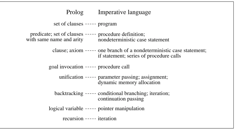
Figure 1: The Correspondence Between Logical and Imperative Concepts

According to Warren, the WAM design was an outcome of his own explorations and was not influenced by this work.

2.2 The Warren Abstract Machine (WAM)

By 1983 Warren had developed the WAM, a structure-copying execution model for Prolog that has become the de facto standard implementation technique [163]. The WAM defines a high-level instruction set that maps closely to Prolog source code. This section concisely explains the original WAM. In particular, the many optimizations of the WAM are given a uniform justification. This section assumes a basic knowledge of how Prolog executes [85, 115, 130] and of how imperative languages are compiled [3].

For several years, Warren’s report was the sole source of information on the WAM, and its terse style gave the WAM an aura of inscrutability. Many people learned the WAM by osmosis, gradually absorbing its meaning. Nowadays, there are texts that give lucid explanations of the WAM and WAM-like systems [4, 85].

2.2.1 The Relationship of the WAM to Prolog and Imperative Languages

The execution of Prolog is a natural generalization of the execution of imperative languages (see Figure 1). It can be summarized as:

Prolog = imperative language + unification

+ backtracking

As in imperative languages, control flow is left to right within a clause. The goals in a clause body are called like procedures. A goal corresponds to a predicate. When a goal is called, the clauses in the predicate’s definition are chosen in textual order from top to bottom. Backtracking is chronological, i.e., control goes back to the most recently made choice and tries the next clause. Hence, Prolog is a somewhat limited realization of logic programming, but in practice its trade-offs are good enough for a logical and efficient programming style to be possible [113].

The WAM mirrors Prolog closely, both in how the program executes and in how the program is compiled:

WAM = sequential control (call/return/jump instructions) + unification (get/put/unify instructions)

+ backtracking (try/retry/trust instructions)

+ optimizations (to use as little memory as possible)

The WAM has a stack-based structure, of which a subset is similar to imperative language execution models. It has call and return instructions and local frame (environment) management instructions. It is extended with instructions to perform unification and backtracking. These form the core of the WAM. Around this core, the WAM has added optimizations intended to reduce memory usage.

Prolog as executed by the WAM defines a close mapping between the terminology of logic and that of an imperative language (see Figure 1). Predicates correspond to procedures. Procedures always have a case statement as the first part of their definition. Clauses correspond to the branches of this case statement. Variables are scoped locally to a clause.3 Goals in a clause correspond to calls. Unification corresponds to parameter passing and assignment. Other features do not map directly: backtracking, the single-assignment nature, and the modification of control flow with the cut operation. Cut is a language feature that increases the determinism of a program by removing choice points.

The WAM is a good intermediate language in the sense that writing a Prolog-to-WAM compiler and a WAM emulator are both straightforward tasks. A compiler and emulator can be built without a deep understanding of the internals of Prolog or the WAM.

3

P Program counter

CP Continuation Pointer (top of return stack) E current Environment pointer (in local stack) B most recent Backtrack point (in local stack) A top of local stack

TR top of TRail H top of Heap

HB Heap Backtrack point (in heap) S Structure pointer (in heap) Mode Mode flag (read or write) A1, A2, ... Argument registers X1, X2, ... temporary variables

Table 1: The Internal State of the WAM

2.2.2 Data Structures and Memory Organization

Prolog is a dynamically typed language, i.e., variables may contain objects of any type at run-time. Hence, it must be possible to determine the type of an object at run-time by inspection.4 In the WAM, terms are represented as tagged words: a word contains a tag field and a value field. The tag field contains the type of the term (atom, number, list, or structure). See [52] for an exhaustive presentation of alternative tagging schemes. The value field is used for different purposes depending on the type: it contains the value of integers, the address of unbound variables and compound terms (lists and structures), and it ensures that each atom has a value different from all other atoms. Unbound variables are implemented as self-referential pointers, i.e., they point to themselves. When two variables are unified, one of them is modified to point to the other.5 _{Therefore it may be necessary to follow a chain of pointers to access a variable’s} value. This is called dereferencing the variable.

Table 1 shows how the internal state of the WAM is stored in registers. The purpose of most registers is straightforward. The HB register caches the value of H stored in the most recent choice point. The S register is used during unification of compound terms (with arguments): it points to an argument being unified. All arguments can be accessed one by one by successively incrementing S. Some instructions have different behaviors during read and write mode unification; the mode flag is used to distinguish between them (see Section 2.2.3). In the original WAM, the mode flag is implicit (it is encoded in the program counter).

The external state (stored in memory) is divided into six logical areas (see Figure 2): two stacks for the data objects, one stack (the PDL) to support unification, one stack (the trail) to support the interaction of unification and backtracking, one area as code space, and one area as a symbol table.

4

Unless the type can be determined at compile-time. 5

trail push-down list (PDL) Three kinds of data objects on stacks

Support for backtracking and unification

code area and symbol table TR PDL P HB local stack E A Yn ... Y2 Y1 CP CE H' TR' BP B' BCP BCE A1 ... Am B Environment Choice point global stack (heap) H S Tn ... T2 T1 F/N Data term

Figure 2: The External State of the WAM

The global stack or heap. This stack holds lists and structures, the compound data

terms of Prolog.

The local stack. This stack holds environments and choice points. Environments (also

known as local frames or activation records) contain variables local to a clause. Choice points encapsulate execution state for backtracking, i.e., they are continuations. A variant model, the split-stack, uses separate stacks for environments and choice points. There is no significant performance difference between the split-stack and the merged-stack models. The merged-stack model uses more memory if choice points are created.

The trail. This stack is used to save locations of bound variables that have to be unbound

The push-down list (PDL). This stack is used as a scratch-pad during the unification of

nested compound terms. Often the PDL does not exist as a separate stack, e.g., the local stack is used instead.

The code area. This area holds the compiled code of a program. It is not recovered on

backtracking.

The symbol table. This area is not mentioned in the original article on the WAM. It

holds various kinds of information about the symbols (atoms and structure names) used in the program. It is not recovered on backtracking. It contains the mapping between the internal representation of symbols and their print names, information about operator declarations, and various system-dependent information related to the state of the system and the external world. Because creating a new entry is relatively expensive, symbol table memory is most often not recovered on backtracking. It may be garbage collected. Systems that manipulate arbitrary numbers of new atoms (e.g., systems with a database interface) must have garbage collection.

It is possible to vary the organization of the memory areas somewhat without changing anything substantial about the execution. For example, some systems have a single data area (sometimes called the firm heap) that combines the code area and symbol table.

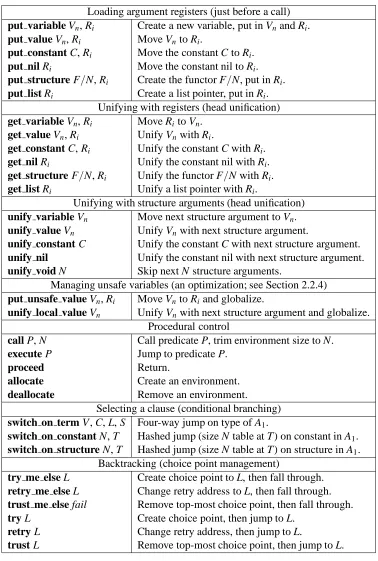
2.2.3 The Instruction Set

The WAM instruction set, along with a brief description of what each instruction does, is summarized in Table 2. Unification of a variable with a data term known at compile-time is decomposed into instructions to handle the functor and arguments separately (see Fig-ures 3 and 4). There are no unify list and unify structure instructions; they are left out because they can be implemented using the existing instructions. The switch on constant and

switch on structure instructions fall through if A1is not in the hash table. The original WAM

report does not talk about the cut operation, which removes all choice points created since entering the current predicate. Implementations of cut are presented in [4, 85]. A variable stored in the current environment (pointed to by E) is denoted by Yi. A variable stored in a register is denoted by Xior Ai. A register used to pass arguments is denoted by Ai. A register used only internally to a clause is denoted by Xi. The notation Viis shorthand for Xior Yi. The notation Ri is shorthand for Xior Ai.

A useful optimization is the variable/value annotation. Instructions annotated with “variable” assume that their argument has not yet been initialized, i.e., it is the first occurrence of the variable in the clause. In this case, the unification operation is simplified. For example, the

get variable X2, A1instruction unifies X2 with A1. Since X2 has not yet been initialized, the

unification reduces to a move. Instructions annotated with “value” assume that their argument has been initialized (i.e., all later occurrences of the variable). In this case, full unification is done.

Sec-Loading argument registers (just before a call)

put variable Vn, Ri Create a new variable, put in Vnand Ri.

put value Vn, Ri Move Vnto Ri.

put constant C, Ri Move the constant C to Ri.

put nil Ri Move the constant nil to Ri.

put structure F=N, Ri Create the functor F=N, put in Ri.

put list Ri Create a list pointer, put in Ri.

Unifying with registers (head unification)

get variable Vn, Ri Move Rito Vn.

get value Vn, Ri Unify Vnwith Ri.

get constant C, Ri Unify the constant C with Ri.

get nil Ri Unify the constant nil with Ri.

get structure F=N, Ri Unify the functor F=N with Ri.

get list Ri Unify a list pointer with Ri.

Unifying with structure arguments (head unification)

unify variable Vn Move next structure argument to Vn.

unify value Vn Unify Vnwith next structure argument.

unify constant C Unify the constant C with next structure argument.

unify nil Unify the constant nil with next structure argument.

unify void N Skip next N structure arguments.

Managing unsafe variables (an optimization; see Section 2.2.4)

put unsafe value Vn, Ri Move Vnto Riand globalize.

unify local value Vn Unify Vnwith next structure argument and globalize.

Procedural control

call P, N Call predicate P, trim environment size to N.

execute P Jump to predicate P.

proceed Return.

allocate Create an environment.

deallocate Remove an environment.

Selecting a clause (conditional branching)

switch on term V, C, L, S Four-way jump on type of A1.

switch on constant N, T Hashed jump (size N table at T) on constant in A1.

switch on structure N, T Hashed jump (size N table at T) on structure in A1.

Backtracking (choice point management)

try me else L Create choice point to L, then fall through.

retry me else L Change retry address to L, then fall through.

trust me else fail Remove top-most choice point, then fall through.

try L Create choice point, then jump to L.

retry L Change retry address, then jump to L.

trust L Remove top-most choice point, then jump to L.

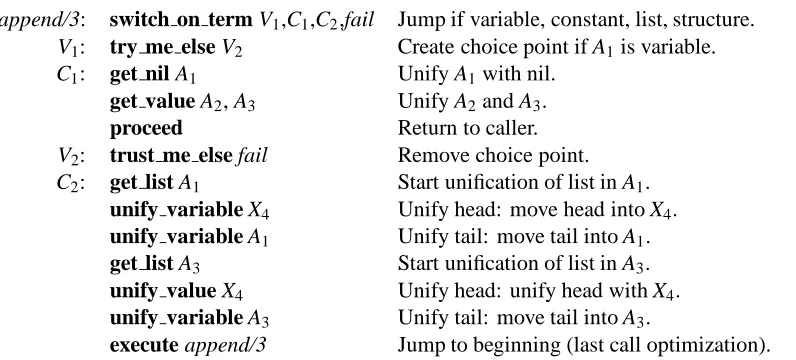
append([], L, L).

append([XjL1], L2, [XjL3]) :- append(L1, L2, L3).

Figure 3: The Prolog Code for append/3

append/3: switch on term V1,C1,C2,fail Jump if variable, constant, list, structure.

V1: try me else V2 Create choice point if A1is variable.

C1: get nil A1 Unify A1with nil.

get value A2, A3 Unify A2and A3.

proceed Return to caller.

V2: trust me else fail Remove choice point.

C2: get list A1 Start unification of list in A1.

unify variable X4 Unify head: move head into X4.

unify variable A1 Unify tail: move tail into A1.

get list A3 Start unification of list in A3.

unify value X4 Unify head: unify head with X4.

unify variable A3 Unify tail: move tail into A3.

execute append/3 Jump to beginning (last call optimization).

Figure 4: The WAM Code for append/3

tion 2.2.5). The switch instruction jumps to the correct clause or set of clauses depending on the type of the first argument. This implements first-argument selection (indexing). The choice point (try) instructions link a set of clauses together. The get instructions unify with the head arguments. The unify instructions unify with the arguments of structures.

The same instruction sequence is used to take apart an existing structure (read mode) or to build a new structure (write mode). The get instructions set the mode flag, which determine whether execution proceeds in read mode or write mode. For example, if get list Ai sees an unbound variable argument, it sets the flag to write mode. If it sees a list argument, it sets the flag to read mode. If it sees any other type, it fails, i.e., it backtracks by restoring state from the most recent choice point. The unify instructions have different behavior in read and write mode. The get instructions initialize the S register and the unify instructions increment the S register.

2.2.4 Optimizations to Minimize Memory Usage

The core of the WAM is straightforward. What makes it subtle are the added optimizations. Because of these optimizations the WAM is extremely memory efficient. For programs with sufficient backtracking, a garbage collector is not necessary. The optimizations are explained in terms of the following classification of memory, from least to most costly to allocate, deallocate, and reuse.

Registers (arguments, temporary variables). These are available at any time without

overhead.

Short-lived memory (environments on the local stack). This memory is recovered on

forward execution, backtracking, and garbage collection.

Long-lived memory (choice points on the local stack, data terms on the heap). This

memory is recovered only on backtracking and garbage collection.

Permanent memory (the code area and symbol table). This memory is recovered only

by garbage collection.

With this classification, the optimizations can be explained as follows.

Prefer registers to memory. There are three optimizations in this category.

– Argument passing. All procedure arguments are passed in registers. This is

im-portant because Prolog is procedure-call intensive. For example, the most efficient way to iterate is through recursion. Backtracking can express iteration as well, but less efficiently.

– The return address. Inside a procedure, the return address of the immediate caller

is stored in the CP register. This optimization is closely related to the leaf routine calling protocol done in imperative language compilers.

– Temporary variables. Temporary variables are variables whose lifetimes do not

cross a call. That is, they are not used both before and after a call. Therefore they may be kept in registers. This definition of temporary variables simplifies and slightly generalizes Warren’s original definition.

Prefer short-lived memory to long-lived memory. There are three optimizations in

this category.

– Permanent variables. Permanent variables are variables that need to survive a

call. They may not be kept in registers, but must be stored in memory. They are given a slot in the environment. This makes it easy to deallocate their memory if they are no longer needed after exiting the predicate (see unsafe variables, below).

– Environment trimming (last call optimization). Environments are stored on

procedure body. This optimization is known as the tail recursion optimization or more accurately, the last call optimization. This is based on the observation that an environment’s space does not need to exist after the last call, since no further computation is done in the environment. The space can be recovered before entering the last call instead of after it returns. Because execution will never return to the procedure, the last call may be converted into a jump. For recursive predicates, this converts recursion into iteration, since the jump is to the first instruction of the predicate. The WAM generalizes the last call optimization to be done gradually during execution of a clause: the environment size is reduced (“trimmed”) after each call in the clause body, so that only the information needed for the rest of the clause is stored. Trimming increases the amount of memory that is recovered by garbage collection.

– Unsafe variables. A variable whose lifetime crosses a call must be allocated an

unbound variable cell in memory (i.e., in an environment or on the heap). If it is sure that the unbound variable will be bound before exiting the clause, then the space for the cell will not be referenced after exiting the clause. In that case the cell may be allocated in the environment and recovered with environment trimming. In the other case one is not sure that the unbound variable will be bound. This leads to the following space-time trade-off. The fastest alternative is to always create the variable on the heap. The most memory-efficient alternative is to create the variable on the environment and just before trimming the environment, to move the variable to the heap if it is unbound. The WAM has chosen the second alternative, and the variable being tested is referred to as an “unsafe variable”.

Prefer long-lived memory to permanent memory. Data objects (variables and

com-pound terms) disappear on backtracking, and hence all allocated memory for them may be put on the heap. In a typical implementation this is not quite true. The symbol table and code area are not put on the heap, because their modifications (i.e., newly interned atoms and asserted clauses) are permanent.

Measurements have been done of the unsafe variable trade-off for Quintus Prolog (see Sec-tion 3.1.4) and the VAM (see SecSec-tion 2.5.1) [76]. Tim Lindholm measured the increase of peak heap usage for Quintus on a set of programs including Chat-80 [161] and the Quintus test suite and compiler. He found that the first alternative increases peak heap usage by 50 to 100% for Quintus (see Section 3.1.4). Because this leads to increased garbage collection and stack shifting, Lindholm concluded that unsafe variables are useful.

Andreas Krall measured the increase of peak heap usage on a series of small and medium-size programs for the VAM, which stores all unbound variables on the heap. He measured increases of from 4% to 26%, with an average of 15%. Because unsafe variables impose a run-time overhead (two comparisons instead of one for the trail check and run-time tests for globalizing variables), Krall concluded that unsafe variables are not useful.

since the run-time overhead is small and the reduction of heap usage is significant.

2.2.5 How to Compile Prolog to the WAM

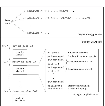
Compiling Prolog to the WAM is straightforward because there is a close mapping between lexical tokens in the Prolog source code and WAM instructions. Figure 5 gives a scheme for compiling Prolog to the WAM. For simplicity, the figure omits register allocation and peephole optimization. This compilation scheme generates suboptimal code. One can improve it by generating switch instructions to avoid choice point creation in some cases. For more information on WAM compilation see [116, 148].

The clauses of predicate p/3 are compiled into blocks of code that are linked together with

try instructions. Each block consists of a sequence of get instructions to do the unification of

the head arguments, followed by a sequence of put instructions to set up the arguments for each goal in the body, and a call instruction to execute the goal. The block is surrounded by

allocate and deallocate instructions to create an environment for permanent variables. The

last call is converted into a jump (an execute instruction) because of the last call optimization (see Section 2.2.4).

2.3 WAM Extensions for Other Logic Languages

Many WAM variants have been developed for new logic languages, new computation models, and parallel systems. This section presents three significant examples:

The CHIP constraint system, which interfaces the WAM with three constraint solvers.

The clp(FD) constraint system, which implements a glass box approach that allows

constraint solvers to be written at the user level.

The SLG-WAM, which extends the WAM with memoization.

2.3.1 CHIP

CHIP (Constraint Handling In Prolog) [2] is a constraint logic language developed at ECRC (see Section 3.1.7 for more information on ECRC). The system has been commercialized by Cosytec to solve industrial optimization problems. CHIP is the first compiled constraint language. In addition to equality over Prolog terms, CHIP adds three other computation domains: finite domains, boolean terms, and linear inequalities over rationals. The CHIP compiler is built on top of the SEPIA WAM-based Prolog compiler. The system contains a tight interface between the WAM kernel and the constraint solvers. The system extends the WAM to the C-WAM (C for Constraint). The C-WAM is quite complex: it has new data structures and over one hundred new instructions. Many instructions exist to solve commonly-occurring constraints quickly.

p(A,B,C) :- q(A,Z,W), r(W,T,B), ..., z(A,X). p(E,F,G) :- k(X,F,P), m(S,T), ...

p(Q,R,S) :- ... ...

choice point

p/3: try_me_else L2

L2: retry_me_else L3

Ln: trust_me_else fail

code for clause 1

code of last clause

allocate

(put arguments)

call q/3

call r/3

deallocate execute z/2

(put arguments)

(put arguments)

Create environment. Unify with caller arguments. (get arguments)

Load arguments and call.

. . .

Load arguments and call.

Remove environment. Last call is a jump.

. . . .

Original Prolog predicate

Compiled WAM code

. . . .

A single compiled clause code for

clause 2

was done with the WAM’s trail condition (see Section 2.2.2). This condition is appropriate for equality constraints, which are implemented by unification in the WAM. For more complex constraints, the condition is wasteful because a variable’s value is often modified several times between two choice points. The CHIP system reduces memory usage by introducing a different trail condition called “time-stamping” [1]. Each data term is marked with an identifier of the choice point segment the term belongs to (see Section 2.3.1). Trailing is only necessary if the current choice point segment is different from the segment stored in the term. Time-stamping is an essential technique for any practical constraint solver.

2.3.2 clp(FD)

The clp(FD) system [29, 40] is a finite domain solver integrated into a WAM emulator. It was built by Daniel Diaz and Philippe Codognet at INRIA (Rocquencourt, France). It uses a glass box approach. Instead of considering a constraint solver as a black box (in the manner of CHIP), a set of primitive operations is added that allows the constraint solver to be programmed in the user language. The resulting system outperforms the hard-wired finite domain solver of CHIP.

In clp(FD), a single primitive constraint is added to the system, namely the range constraint X

in R, where X is a domain variable and R is a range (e.g., 1..10). Instead of just using constant

ranges, the idea is to introduce what are known as indexical ranges, i.e., ranges of the form

f(Y)..g(Y) or h(Y) where f(Y), g(Y), and h(Y) are functions of the domain variable Y. A set

of these functions that do local propagation is built-in. For example, the system provides the constraints X in min(Y)..max(Y) and X in dom(Y) with the obvious meanings. Arithmetic constraints such as X=Y+Z and boolean constraints such as X=Y and Z can be written in terms of indexical range constraints.

Indexical range constraints are smoothly integrated into the WAM by providing support for domain variables and suspension queues for the various indexical functions [40]. The time-stamping technique of CHIP is used to reduce trailing.

2.3.3 SLG-WAM

Memoization is a technique that caches already-computed answers to a predicate. By adding memoization to Prolog’s resolution mechanism, one obtains an execution model that can do both top-down and bottom-up execution. For certain algorithms, this model executes simple logical definitions with a lower order of complexity than a pure top-down execution would. For example, the recursive definition of the Fibonacci function runs in linear time rather than exponential time. More realistic examples are parsing and dynamic programming.

implemented in XSB, and is much faster than deductive database systems [132]. An important source of overhead is the complex trail: it is a linked list whose elements contain the address and old contents of a cell.

2.4 Beyond the WAM: Evolutionary Developments

The WAM was a large step towards the efficient execution of Prolog. From the viewpoint of theorem proving, Prolog is extremely fast. But there is still a large gap between the efficiency of the WAM and that of imperative language implementations. As people started using Prolog for standard programming tasks, the gap became apparent and people started to optimize their systems. This section discusses the gap and some of the clever ideas that have been developed to close it.

2.4.1 Chinks in the Armor

This section lists the limits to Prolog performance and their causes.

WAM instructions are too coarse-grained to perform much optimization. For example,

many WAM instructions perform an implicit dereference operation, even if the compiler can determine that such an operation is unnecessary in a particular case. In practice, dereference chains are short: dynamic measurements on real programs show that two thirds are of length zero (no memory reference is required), one third are of length one, and <1% are of length two or greater [145]. Despite these statistics, dereferencing is

expensive. For example, Aquarius on the VLSI-BAM, a high-performance system with hardware support, spends 9% of its total execution time doing dereferencing [152].

The majority of predicates written by human programmers are intended to give at most

one solution, i.e., they are deterministic. These predicates are in effect case statements, yet they are too often compiled in an inefficient manner using the full generality of backtracking (which implies saving the machine state and repeated failure and state restoration). The WAM’s first-argument selection is inadequate to compile these predi-cates efficiently (see Section 2.4.3). Measurements of Prolog applications support this assertion:

– Tick shows that shallow backtracking (backtracking from clause to clause within a

single predicate) dominates even for well-written deterministic programs. Choice point references constitute about half (45–60%) of all data references [143].

– Touati and Despain show that at least 40% of all choice point and fail operations

can be removed through optimization [145].

The single-assignment nature of Prolog (i.e., a variable can only be assigned one value

problem, is a special case of the general problem of efficiently representing state modi-fication in logic. It is impossible to use large data structures with the same efficiency as in procedural languages unless the compiler is able to introduce destructive assignment (overwriting of memory locations) in the implementation. Section 5.1 gives suggestions on how to get around this problem.

Prolog has dynamic typing (variables may contain values of any type) and dynamic

memory allocation (all data objects are allocated at run-time). Both of these cost execution time. They should be compiled statically wherever possible.

Programming style has a large effect on a program’s efficiency. Prolog programming is

at a high level of abstraction, so it hides many details of the implementation from the programmer, making it difficult to improve efficiency when it is important to do so. For example, adding a single cut can make the difference between a program that runs fast and one that thrashes. This is possible even if the cut does not change the operational semantics of the program. The thrashing behavior is caused by a pile-up of choice points during deterministic (forward) execution. Because the choice points encapsulate execution states that remain accessible through potential backtracking, their memory is not recovered by garbage collection.

The apparent need for architectural support. So-called “general-purpose” architectures

are in fact optimized for imperative languages and number crunching. To run Prolog equally well, either the compiler must do more work, or conceivably the architecture should be modified. Some experiments have been done with architectures optimized for Prolog (among others, the PSI-II, KCM, and VLSI-BAM, see Section 3.2), but the true architectural needs of Prolog are a moving target. They depend on the execution model and the sophistication of the compiler. As better compilers have been developed, the perceived architectural needs of Prolog have been getting smaller and smaller. One need likely to stay for a long time is a fast memory system. Prolog’s dynamic nature requires frequent pointer dereferencing. There are no compilation techniques on the horizon that are likely to reduce the resulting need for a fast memory system (see Section 5.1).

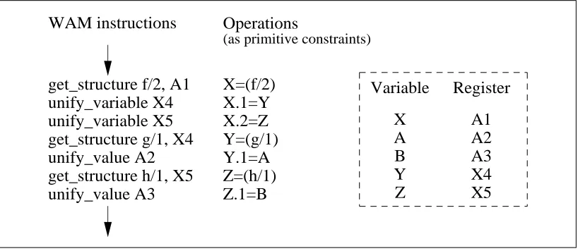
2.4.2 How to Compile Unification: The Two-Stream Algorithm

This section presents the two-stream unification algorithm, an elegant scheme for compiling unification that is more efficient than the WAM for native code implementation. Rough measurements comparing unification times of the VLSI-PLM (a microcoded WAM) and the VLSI-BAM (see Section 3.2.3) show a speedup factor of two to three [153] in favor of the latter. This algorithm was independently reinvented at least four times by different people at about the same time: Mohamed Amraoui at the Universit´e de Rennes I [8], Andr´e Mari¨en and Bart Demoen at BIM and KUL [86, 88], Kent Boortz at SICS [16], and Micha Meier at ECRC [94]. Write mode propagation was discussed earlier by Andrew Turk [146].

get_structure f/2, A1 unify_variable X4 unify_variable X5 get_structure g/1, X4 unify_value A2 get_structure h/1, X5 unify_value A3

X=(f/2) X.1=Y X.2=Z Y=(g/1) Y.1=A Z=(h/1) Z.1=B

Variable

X A B Y Z WAM instructions Operations

(as primitive constraints)

Register

A1 A2 A3 X4 X5

Figure 6: The WAM Compilation of the Unification X=f(g(A),h(B))

Functor and argument constraints correspond to the get and unify instructions in the WAM. An important advantage of the primitive constraint representation over the WAM is that the constraints may be executed in any order. In addition to providing a powerful conceptual description of the WAM, primitive constraints are useful in compiling more advanced logic languages [6, 84, 117].

The WAM compiles unification as a single sequence of instructions (see Figure 6). This has several problems:

Write mode is not propagated to subterms. For example, the unification X=f(g(a))

is compiled as X=f(T), T=g(a). These two unifications are compiled independently. If X is unbound, the fact that T is created as an unbound variable in the first unification is not propagated to the second unification. This means a superfluous dereference, a superfluous trail check, and a superfluous binding.

Instructions have modes. All instructions have two modes of execution, read mode and

write mode. The current mode is stored in a global mode flag, which is set in get list and

get structure instructions and tested in all unify instructions. Some implementations

(e.g., the intended implementation of the original WAM report, and Quintus) encode the mode flag in the program counter, which avoids the testing overhead.

Poor translation to native code. The straightforward method for generating native code

is to macro-expand the WAM instructions. This means that the read and write mode parts are interleaved, which results in many jumps. This is less of a problem on a microcoded machine since microcode jumps are often free (the destination address is part of the microword).

if S=1 jump L'

Selectively executed

subsequence

Sequence of

instructions

set S

←

0

set S

←

1

jump L

L:

L':

W stream

R stream

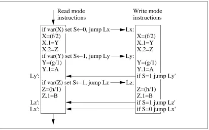
Figure 7: How to Execute a Particular Subsequence with Low Overhead

two streams one avoids superfluous operations while keeping a linear code size. The practical problems that remain are how to configure the instructions so they work correctly despite being jumped to from different places, and how to minimize bookkeeping overhead for the jumps.

Figure 7 illustrates a technique to execute any subsequence of a main instruction sequence with very little overhead. The idea is to give the main sequence an identifier (say, the integer 0) and the subsequence a different identifier (say, the integer 1). Then a single conditional jump is all that is required. If the subsequence is non-contiguous, then a single conditional jump to the next segment is needed per contiguous segment of the subsequence. If more than one subsequence has to be selected, then a unique identifier is needed for each one. The subsequences may be overlapping.

With the idea of selective execution in mind, arrange the primitive constraints of the term according to a depth-first traversal of the term (Figure 8). The resulting sequence satisfies the property that each subterm corresponds to a contiguous sequence of instructions. This is all one needs to implement the algorithm. At run-time, unification follows the read mode stream, and selectively executes contiguous parts of the write mode stream for subterms to be created.

Ly':

Lz':

Lx':

Lx:

Ly:

Lz:

X=(f/2)

X.1=Y

X.2=Z

Y=(g/1)

Y.1=A

if S=1 jump Ly'

Z=(h/1)

Z.1=B

if S=1 jump Lz'

if S=0 jump Lx'

if var(X) set S

←

0, jump Lx

X=(f/2)

X.1=Y

X.2=Z

if var(Y) set S

←

1, jump Ly

Y=(g/1)

Y.1=A

if var(Z) set S

←

1, jump Lz

Z=(h/1)

Z.1=B

Read mode

instructions

Write mode

instructions

Figure 8: The Two-Stream Compilation of the Unification X=f(g(A),h(B))

conditional jump (changing the condition from “=” to “”). In Figure 8, the two conditional

jumps if S=1 jump Lz’ and if S=0 jump Lx’ can be rewritten as the single jump if S0 jump

Lz’. To collapse the maximum number of jumps, reorder the arguments of all subterms to unify the most complex subterms last.

The advantages of the two-stream algorithm are:

Low overhead. The bookkeeping overhead is a small constant factor. The only

book-keeping is the set of jumps and register moves needed to manage the selective execution of subsequences. This is small compared to the work done in the primitive constraints. There is no explicit mode flag.

Downward propagation of write mode. The write mode of a term is propagated at

compile-time to all of its subterms. There are no superfluous dereferences, trail checks, or bindings.

Upward propagation of read mode. The read mode of a term is propagated at

compile-time to its siblings and ancestors.

Linear code size. This contrasts with the algorithm of [150], which expands all cases

without any sharing. That algorithm has zero bookkeeping overhead, but exponential code sizes occur in practice.

dou-ble that of the WAM, but the instructions themselves have less than half the complexity. The primitive constraints of Figure 8 are expanded differently in the read mode and write mode streams. Essentially, the internal operations of the WAM instructions have been made visible and arranged in an efficient order. There are no jumps inside the primitive constraints, but only between them, and then only when it is necessary to choose between read and write mode.

2.4.3 How to Compile Backtracking: Clause Selection Algorithms

This section surveys the clause-selection algorithms that have been developed since the WAM. The WAM supports first-argument selection. It has instructions that can choose clauses based on the main functor of the first argument. If all of a predicate’s clauses contain different main functors, then a hash table can be constructed and calling the predicate will avoid a choice point creation when the first argument is not a variable. In the general case, predicates can be compiled to create at most one choice point between entry and the execution of the first clause [24, 148]. The original WAM report describes a two-level indexing scheme which creates up to two choice points [163].

Many programs cannot profit from first-argument selection. For example, selection may depend on more than one argument. The following example is extracted from an actual program. The first two arguments are integer inputs, the third is an output (all numbers are in base two):

get relop(2’001, 2’001, 2’000). get relop(2’001, 2’010, 2’011). get relop(2’001, 2’011, 2’000). ... 33 more clauses ...

The second example is a predicate in which selection depends on arithmetic comparisons instead of unification only:

max(A, B, C) :- AB, C=B.

max(A, B, C) :- A>B, C=A.

In general, selection is possible if the compiler can determine that only a subset of the clauses in the definition can possibly succeed, given some particular argument types at the call. An appropriate definition of type is given in Section 2.4.5.

An ideal clause-selection algorithm would generate code that has the following properties:

It takes advantage of argument types to try only the clauses that can possibly succeed.

It avoids all useless choice point creations.

It creates choice points incrementally, i.e., choice points contain only that part of the

execution state that needs to be saved.

Its performance degradation is gradual if insufficient type information is known.

There is no published algorithm that satisfies all these conditions. There are published algo-rithms that satisfy some of the conditions and do better clause selection than the WAM. Several algorithms create a selection tree or graph, i.e., a series of tests that determine which subset of clauses to try given particular arguments (e.g., [167]). Generating a naive selection tree may result in exponential code size for predicates encountered in real-world programs. The following algorithms are noteworthy:

Van Roy, Demoen, and Willems [149] present a compilation algorithm that generates

a naive selection tree and creates choice points incrementally. The algorithm compiles clauses with four entry points, depending on whether or not there are alternative clauses, and whether or not a previously executed clause has created a choice point. The algorithm was not implemented.

Carlsson [25] has implemented a restricted version of the above algorithm in SICStus

Prolog. Meier [92] has done a similar implementation in KCM-SEPIA. Choice point creation is split into two parts. The try and try me else instructions are modified to create a partial choice point that only contains P and TR. A new instruction, neck, is added. If a partial choice point exists when neck is executed, then the remaining registers are filled in. Two entry points are created for each clause: one when there are alternative clauses, and one where there are none. A neck instruction is only included in the first case. In SICStus, this algorithm results in a performance improvement of 7% to 15% for four large programs, at a cost of a 5% to 10% increase in code size.

Hickey and Mudambi [61] present compilation algorithms to generate a tree of tests

and to minimize work done in backtracking. One of their selection algorithms results in a tree that has a quadratic worst-case size. They improve choice point management. The try instruction only stores registers needed in clauses after the first clause. The

retry and trust instructions restore only those registers needed in the clause and remove

the registers not needed in subsequent clauses. The latter operation lets the garbage collector recover more memory. The technique of improved choice point management was independently invented earlier by Andrew Turk [146] and later by Van Roy [153]. The technique has not yet been quantitatively evaluated.

Kliger [71, 72] presents a compilation algorithm that generates a directed acyclic graph

The Aquarius system [153, 154] produces a selection graph for disjunctions containing

three kinds of tests: unifications, type tests, and arithmetic comparisons. It uses heuristics to decide which tests to do first and whether to use linear search or hashing for table lookup. The nodes in the graph partition the tests occurring in the predicate. Each node corresponds to a subset of these tests. Unifications are only used as tests if it can be deduced from the predicate’s type information that they will be executed in read mode. The type enrichment transformation adds type information to a predicate that lacks it. The performance of the resulting code is therefore always at least as good as first-argument selection. The factoring transformation allows the system to take advantage of tests on variables inside of terms, by performing the term unification once for all occurrences of the term. The problem with Aquarius selection is similar to that of the naive selection tree: if too much type information is given, then the selection graph may become too large.

The Parma system [140] uses techniques similar to Aquarius. It produces efficient

indexing code for the same three kinds of tests. To improve the clause selection, Parma uses transformations analogous to type enrichment and factoring. It uses optimal binary search for table lookup. Taylor’s dissertation discusses how to choose between linear search, binary search, jump tables, and hashing.

2.4.4 Native Code Compilation

One way to improve the performance of a WAM-based system is to add instructions. For example, instructions can be added to do efficient arithmetic and to index on multiple arguments. Common instruction sequences can be collapsed into single instructions. This is quick to implement, but it is inherently a short-term solution. As the number of instructions increases, the system becomes increasingly unwieldy.

The main insight in speeding up Prolog execution is to represent the code in terms of simple instructions. The first published experiments using this idea were done in 1986 by Komatsu et al [73, 135] at IBM Japan. These experiments gave the first demonstration that specialized hardware is not essential for high-performance execution of Prolog. Compilation is done in three steps. The first step is to compile Prolog into a WAM-like intermediate code. In the second step the WAM-like code is translated into a directed graph. The graph is optimized using rewrite rules. In the final step, the result is translated into PL.8 intermediate code and compiled with an optimizing compiler. For several small programs, this system demonstrated a fourfold performance improvement using mode hints given by the programmer.

BAM Code SPARC Code procedure(append/3). test(ne,tlst,r(0),L1). L2: pragma(align(r(0),2)). pragma(tag(r(0),tlst)). move([r(0)],r(3)). pragma(tag(r(0),tlst)). move([r(0)+1],r(0)). pragma(tag(r(2),tvar)). move(tlst^r(h),[r(2)]). pragma(push(term(2))). pragma(push(cons)). push(r(3),r(h),1). move(tvar^r(h),r(2)). adda(r(h),1,r(h)). test(eq,tlst,r(0),L2). L1: equal(r(0),tatm^[],fail). pragma(tag(r(2),tvar)). move(r(1),[r(2)]). return. ... L2:

add %l3, 0, %o0 add %l3, 8, %l3 ld [%g1-1], %g4 ld [%g1+3], %g1 st %g4, [%l3-9] add %l3, -5, %g3 and %g1, 3, %o0 cmp %o0, 1 be,a L2

st %l3, [%g3] ...

Kernel Prolog Code

A,L1 = r(0) = %g1 C,L3 = r(2) = %g3 X = r(3) = %g4 (heap) r(h) = %l3 (temp) %o0

tlst = 1 tvar = 0

r(h) has tlst tag Registers: Tags: append(A,B,C) (cons(A) -> A=[X|L1], C=[X|L3], append(L1,B,L3) ; A=[], B=C ).

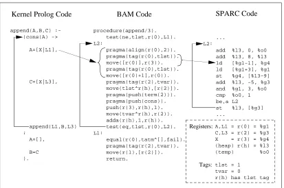
Figure 9: The Aquarius SPARC Code for append/3 in Naive Reverse

performance results for Parma on a MIPS processor. The first results for Aquarius were presented in [63], which describes the VLSI-BAM processor and its simulated performance. A second paper measures the effectiveness of global analysis in Aquarius [152]. Both the Parma and Aquarius systems vastly outperform existing implementations. They prove the effectiveness of compiling directly to a low-level instruction set using global analysis to help optimize the code.

An important idea in both systems is uninitialized variables. An uninitialized variable is defined to be an unbound variable that is unaliased, i.e., there is exactly one pointer to it. An uninitialized variable can be represented more efficiently than a standard WAM variable. Beer first proposed the idea of uninitialized variables after he noticed that most unbound variables in the WAM are bound soon afterwards [12]. For example, this is true for output arguments of predicates. WAM variables are created as self-referencing pointers in memory, and need to be dereferenced and trailed before being bound. This is time-consuming. Beer represents variables as pointers to memory words that have not been initialized. He introduces several new tags for these variables and keeps track of them at run-time. The creation of uninitialized variables is simpler and they do not have to be dereferenced or trailed. Binding them reduces to a single store operation. In Parma and Aquarius, these variables are derived by analysis at compile-time. They use the same tag as other variables.

due to Bruce Holmer. This variable is an output that is passed in a register. No memory is allocated for uninitialized registers, unlike standard uninitialized variables. This reduces the space advantage of unsafe variables. The use of uninitialized registers allows Aquarius to run recursive integer functions faster than popular implementations of C [154].6 In principle, all uninitialized variables can be transformed into uninitialized registers. In practice, to avoid losing last call optimization (see Section 2.2.4) only a subset is transformed [153]. The trade-off with last call optimization has not yet been studied quantitatively.

Figure 9 shows the Aquarius intermediate codes (kernel Prolog and BAM code) and the SPARC code generated for append/3 in naive reverse. See Figures 3 and 4 for the Prolog source code and WAM code. Kernel Prolog is Prolog without syntactic sugar and extended with efficient conditionals, arithmetic, and cut.

The BAM (Berkeley Abstract Machine) is an execution model with a memory organization similar to the WAM. The BAM defines a load-store instruction set supplemented with tagged addressing modes, pragmas, and five Prolog-specific instructions (dereference, trail, general unification, choice point manipulation, and environment manipulation). Pragmas are not executable but give information that improves the translation to machine code.

In the SPARC code, tags are represented as the low two bits of a 32-bit word. This is a common representation that has low overhead for integer arithmetic and pointer dereferencing [52]. The tag of a pointer is always known at compile-time (it is put in a pragma). When following a pointer, the tag is subtracted off at zero cost with the SPARC’s register+displacement

addressing mode. The compiler derives the following types for append/3:

mode((append(A,B,C) :-ground(A), rderef(A), ground(B), rderef(B), uninit(C))).

An uninitialized argument is represented by uninit. A ground argument contains no unbound variables. A recursively dereferenced (rderef) argument is dereferenced and its arguments are recursively dereferenced. This type generalizes the DEC-10 mode:

:- mode append(++, ++, ).

which states that the first two arguments are ground and the last argument is an unbound variable.

6

2.4.5 Global Analysis

Global analysis of logic programs is used to derive information to improve program execution. Both type and control information can be derived and used to increase speed and reduce code size. The analysis algorithms studied so far are all instances of a general method called abstract interpretation [34, 35, 69]. The idea is to execute the program over a simpler domain. If a small set of conditions are satisfied, this execution terminates and its results provide a correct approximation of information about the original program. Le Charlier et al [80, 81] have performed an extensive study of abstract interpretation algorithms and domains and their effectiveness in deriving types. Getzinger [50] has recently presented an extensive taxonomy of analysis domains and studied their effects on execution time and code size.

Since Mellish’s early work in 1981 and 1985 [96, 98], global analysis has been considered useful for Prolog implementation. This section summarizes the work that has been done in making analysis part of a real system. By type we denote any information known (at compile-time or at run-compile-time) about a variable’s value at run-compile-time. A mode is a restricted type that indicates whether the variable is used as an input (nonvariable) or an output (unbound variable). Useful types include argument values, compound structures, dependencies between variables, and operational information such as the length of dereference chains (see also Sections 2.4.6 and 5.1).

In 1982, Lee Naish performed an experiment with automatically generated control information for MU-Prolog [106]. Control information is all information related to the execution order of a program’s procedures. The MU-Prolog interpreter supports wait declarations. A “wait” declaration defines a set of arguments of a predicate that may not be constructed by a call (i.e., unified in write mode). When a call attempts to construct a term in any of these arguments, then the call delays until the argument is sufficiently instantiated so that no construction is done (i.e., the argument is unified in read mode). This provides a form of coroutining. The automatic generation of “wait” declarations is based on a simple heuristic: to delay rather than guess one of an infinite number of bindings.7A “wait” declaration is inserted for each recursive call that does not progress in its traversal of a data structure. This algorithm was implemented and tested on some small examples. It significantly reduces the programmer’s burden in managing control, but it does not always help: if the clause head is as general as the recursive call then no “wait” declaration is generated, even though one might be necessary.

A later system, NU-Prolog, supports when declarations. These are both more expressive and easier to compile into efficient code (see Section 3.1.3). A “when” declaration is a pattern containing a term with optional variables and a nested conjunction and/or disjunction of nonvariable and ground tests on these variables. Variables may not occur more than once in the term. A “when” declaration is true if unification between the term and the call succeeds and does not bind any variables in the call. A call will delay until its “when” declarations are true. This is called one-way unification or matching. NU-Prolog contains an analyzer that derives “when” declarations.

7