University of Warwick institutional repository: http://go.warwick.ac.uk/wrap
This paper is made available online in accordance with publisher policies. Please scroll down to view the document itself. Please refer to the repository record for this item and our policy information available from the repository home page for further information.
To see the final version of this paper please visit the publisher’s website. Access to the published version may require a subscription.
Author(s): Karsten Matthies and Florian Theil
Article Title: Validity and Failure of the Boltzmann Approximation of Kinetic Annihilation
Year of publication: 2010 Link to published article:
http://dx.doi.org/10.1007/s00332-009-9049-y
LONG-TIME VALIDITY OF THE GAINLESS HOMOGENEOUS BOLTZMANN EQUATION
KARSTEN MATTHIES AND FLORIAN THEIL
Abstract. This paper introduces a new method to show the validity of a continuum description for the deterministic dynamics of many interacting particles. Here the many particle evolution is analyzed for a hard sphere flow with the addition that after a collision the collided particles are removed from the system. We consider initial conditions, which are Poisson distributed according a spatially homogeneous velocity densityf0(v) that has finite mass and variance (kinetic energy) and does not concentrate mass on lines. As-suming finite energy and no concentration properties onf0, the homogeneous Boltzmann equation without gain term is derived for arbitrary long times in the Boltzmann-Grad scaling. A key element is a novel description of the many particle flow by a hierarchy of trees which encode the possible collisions. The occurring trees are shown to have favorable properties with a high probability, allowing to restrict the analysis to a finite number of interacting particles, enabling us to extract a single-body distribution. A counter-example is given for a concentrated initial densityf0even to short-term validity.
The derivation of the continuum models of mathematical physics from atomistic descrip-tions is a longstanding and fundamental problem, see problem six in [Hil00]. This ar-ticle is the first of a series of papers ([MT07a], [MT07b], [MT07c]) where we propose and develop a new method that allows us to derive and justify effective continuum limits as scaling limits of large interacting particle systems. In particular we can con-front a fundamental challenge in statistical mechanics: The emergence of irreversible macroscopic behavior generated by deterministic reversible Hamiltonian micro-evolution. For earlier work, which was mostly restricted to short times or linear equations, see [Gal70, Lan75, Spo78, BBS83, Spo91, CIP94] and references therein.
We consider the effective Hamiltonian evolution ofn hard balls (u(i, t), v(i, t))∈Td×Rd,
i ∈ {1. . . n} for d = 2,3 with diameter a. We are mostly interested in the effective evolution generated by the kinetic limit wherentends to infinity, the initial values (u(i, t= 0), v(i, t= 0)) are iid random variables with lawf0 ∈P M(Td×Rd) whereTd denotes the
d-dimensional unit-torus. The diameteraof the particles is linked tonby the Boltzmann-Grad relation
(1) lim
n→∞na
d−1 = 1.
If the particles interact with each other via a hard-core potential it is expected that for every open set Ω ⊂ Td ×Rd at every time t the number of particles in Ω divided by
the total number of particles converges to RΩ dft(u, v). The time-dependent probability
measure f solves the nonlinear Boltzmann equation
(2) ∂tf+v·∂uf =Q+[f, f] +Q−[f, f],
whereQ+is the gain-term,Q− is the loss term andQ=Q++Q−is the collision operator.
The collision kernels correspond to a situation of completely independent particles with densityf(u, v, t), which collide at positionuwith a probability depending on the velocities v and v0 of the colliding particles. The colliding particles change their velocities from v
and v0 to v
∗ and v0∗, so there is a loss in the density at (u, v) and (u, v0) and a gain at
(u, v∗) and (u, v∗0).
The analysis of (2) is nontrivial and culminated in the celebrated paper by Lions and DiPerna ([DL90]) where existence of renormalized solutions is rigorously established for the first time. The mathematical challenges are a result of the subtle interplay between the transport termv·∂uf and the nonlinear gain-termQ+[f, f]. If either of the two terms
is not present the analysis of the Boltzmann equation simplifies considerably.
In this paper we will drop both terms and consider the conceptually simplest situation where the motion of each particle moves with constant velocity until it interacts with another particle. After the collision the collided particles are removed from the system. The transport term can be dropped by considering spatially homogenous initial data. Two of the remaining three scenarios will be treated in [MT07a] and [MT07b]. The analysis of the case where both the transport-term and the gain-term are present requires the development of new compactness results for this type of many-body system.
First we will derive the mean-field theory for a single particle which consists of a ho-mogeneous Boltzmann equation without gain-term. We prove rigorously that the weak-* limit of the empirical densities indeed satisfies the mean-field theory, provided that f0 ∈M+(Rd) has finite total mass and kinetic energy
(3)
Z
Rd
(1 +|v|)2df0(v) =Kini <∞
and does not concentrate mass on single velocity directions, i.e.
(4)
Z
ρ(v,ν)
df0(v0) = 0 for all v ∈Rd, ν ∈Sd−1,
whereρ(v, ν) =v+Rν is a line. The proof constitutes the core of this article as it is based
on new ideas that have not appeared in the literature yet. Instead of extracting the single-body density directly from the complicated n-body evolution we insert an intermediate layer: trees which encode the collision history of the individual particles. Our trees solve in the case of hard-ball dynamics in the Boltzmann-Grad limit many difficulties that haunted previous attempts to answer the question how to extract single-body densities from many-body evolution:
(1) It is not difficult to construct the limiting distribution P of the trees which is obtained by ignoring correlations caused by rare events such as recollisions. (2) We can extract the single-body density ft from the distribution of the trees in
a relatively simple way. This amounts to distinguishing between the observed degrees of freedom (odof) and the background noise which drives the evolution of the odof.
(3) The convergence of the empirical distribution ˆP to the limiting distributionP can be derived on a set of good trees G. The formula for P is so simple that it is not hard to construct a reasonably sharp upper bound P(Gc) = o(1) as a tends to
0. The combination of these two facts constitutes a rigorous justification of the mean-field theory.
In particular the last point is of crucial importance if one attempts to extract the laws of thermodynamics from deterministic systems with random initial conditions.
For this reason we will first study the tree-equivalent of the Boltzmann-equation: the limiting distribution of trees which is obtained by ignoring correlations. We will show how time plays the role of a parameter which resembles temperature in equilibrium statistical mechanics (equation (20)). Furthermore, the extraction of the single-body distribution will reveal the conceptual link between the Boltzmann equation and the distribution of the trees (Proposition 13).
The hard part of the analysis consists in step (3) where we have to bound the probability of bad trees (Proposition 17).
In Section 3 we will discuss an example which shows that assumption (4) cannot be dropped without losing the approximation property of the Boltzmann equation. We demonstrate that for arbitrarily short but finite times the weak-* limit of the empirical density is not consistent with the mean-field theory. In the last section, we collect some proofs, which are not immediately needed in the understanding and the development of the concepts of this article. An appendix with a list of frequently used notation is included.
1. Main result
For spatially homogeneous initial data the mean-field theory leads to Boltzmann equations without transport and gain term
(5) f˙=Q−[f, f], ft=0 =f0,
where Q−[f, f](v) = −
R
Rddf(v0)κd|v −v0|f(v) is the loss term with κd the volume of
d−1 dimensional unit-ball, in particular κ2 = 2, κ3 =π.
We prove a somewhat weaker statement than the one stated in the introduction. The number of particles n is a random number, the law of n is a Poisson-distribution with intensity N =a1−d. This assumption entails that nad−1 is a sequence of random numbers
such that lima→0nad−1 = 1 almost surely if a assumes only a countable set of values
which converges to 0 quickly enough. On the other hand, if the number of particles is determined uniquely by a it is expected that the same result holds but the additional knowledge introduces correlations which are not dealt with in this work.
On the atomistic level we consider n particles with initial values (u0(i), v0(i))∈Td×Rd,
i= 1. . . n, which evolve by Newtonian dynamics
u(a)(i, t= 0) =u0(i), v(a)(i, t= 0) =v0(i),
˙
u(a)(i, t) =v(a)(i, t), v˙(a)(i, t) = 0.
(6)
For each t ∈ [0,∞), i ∈ {1. . . n} there exists a unique scattering state βi(a)(t) ∈ {0,1}
which satisfies the implicit relation
β(a)(i, t) =
(
1 if dist(zi, zi0, s)≥aβ(a)(i0, s) for all s∈[0, t), i0 6=i,
0 else (7)
with a modified distance function to ignore initial intersections
(8) dist((u, v),(u0, v0), s) =|u−u0 +s(v−v0)|+aχ[0,a](|u−u0|).
Definition 1 (Poisson point processes). Let Ωbe a measure space. The random variable
z ∈ ∪∞
n=0Ωn forms a Poisson point process with density µ∈M+(Ω) if
Prob(z ∈Ωn) =e−µ(Ω)µ(Ω)
n
n! , law(zi) =µ/µ(Ω),
andz1, . . . , znare independent. The law of the Poisson point process is denoted byProbppp.
Theorem 2. (Justification of the gainless Boltzmann equation) Letf0 ∈P M+(Rd), d≥2 be a momentum density that satisfies (3, 4) and let for each N > 0 the random variable
(u0, v0) ∈ ∪∞n=0(Td ×Rd)n be a Poisson point process with intensity N(1Td ⊗f0). Let n particles with initial values(u0(i), v0(i))∈Td×Rd, i= 1. . . n evolve by (6). IfN depends on a such that
N ad−1 = 1,
then for each t ∈[0,∞), ε >0, measurable A⊂Td ×Rd
lim
a→0Probppp
1 N#
i∈ {1. . . n} | (u(a)(i, t), v(a)(i, t))∈A and β(a)(i, t) = 1
(9)
−
Z
A
dudft(v) > ε
= 0,
where f : [0,∞)→M+(Rd) is the unique solution of (5).
The assumption thatRRddf0(v) = 1 is not necessary. We make it because it simplifies the
notation in the proof which can be found at the end of Section 2.
Stronger results can be obtained, if the rate at which a tends to 0 is controlled.
Corollary 3. Under the same assumptions as above there exists a subsequence of diam-eters ak such that limk→∞ak = 0 and
(10) 1
Nk n X
i=1
βi(ak)(t)δ(· −(u(
ak)(i, t), v(ak)(i, t)))* f∗
t
weak-* in M(Td ×Rd) as k → ∞.
It is not hard to obtain more explicit subsequences such as ak = k−p e.g. for p > 1 if
additional regularity assumptions forf0 are made. The proof of Corollary 3 is given after
the proof of the theorem.
Assumption (4) does not exclude the possibility that f0 is concentrated on lower
dimen-sional subsets, for example the uniform distribution on the sphere Sd−1 is admissible, i.e.
f0 satisfies
(11)
Z
ϕ(v) df0(v) :=
1
Hd−1(Sd−1)
Z
Sd−1
ϕ(v) dHd−1(v),
for all testfunctions ϕ∈Cc(Td×Rd), where Hd is the d-dimensional Hausdorff-measure.
The approach due to Lanford [Lan75] which uses the BBGKY-hierarchy to derive this equation from the Hamiltonian evolution relies heavily on analytic properties in time and high regularity of f.
As a motivation for our analysis, we give an example why the previous is restricted to short times, even for the gainless case. Let us assume thatf0 is given by (11). Solutionsf
of (5) which satisfyft=0 =f0 can be written asft =ρ(t)f0, where ρsatisfies the ordinary
differential equation
(12) ρ˙ =−γρ2, ρ(t= 0) = 1.
The collision rate γ(v) = R κd|v−v0|df0(v0) is constant for v ∈Sd−1, the support of f0,
since f0 is invariant under rotations.
The solution of system (12) is given by
(13) ρ(t) = 1
1 +γt.
As the geometric series P∞k=0(−γt)k diverges if γ|t| >1 formula (13) shows that writing
f as a power series in t is restricted to small times. Although the solution is a perfectly smooth and bounded function for t ∈ [0,∞) the approach is haunted by the singularity at t =−1
γ. In this particular example, an alternative could be restarting the procedure
at small positive time using suitable a-priori estimates.
Never the less such an approach is not extendable to other cases. For this reason we develop a different method to study the coarse-grained many-body dynamics. Further-more, we will analyze effects due to concentration by a Taylor expansion in time of ft in
Section 3
2. Proof of Theorem 2
2.1. The hierarchy of evolutions. Instead of expanding ρ into a power-series in tand matching coefficients in a first step, we replace the initial value problem (5) by an infinite system using general initial distribution without concentrations
(14) f˙k =Q−[fk−1, fk], ft=0,k =f0.
SinceQ− is quadratic, for fixedkthe integro-differential equation (14) is in fact linear and
non-autonomous. We can therefore work with the mathematically much more convenient mild formulation. The differential equation completely decouples in v and the equation for each v is a scalar linear nonautonomous ODE, which can be directly integrated to
(15) ft,k = exp(−
Rt
0L[fs,k−1] ds)f0,
where L[f](v) = κd R
df(v0)|v−v0|. We observe that df
t,k(v) is absolutely continuous
with respect to df0(v) due to the decoupling in v.
Lemma 4. Let f0 ∈M(1+|v|)2 thenfk converges in Cρ0([0,∞), M1+|v|) tof for some ρ >0
and f ∈C1([0,∞), M
1+|v|) is the unique solution of (5).
ByM1+|v|andM(1+|v|)2 we mean the set of Radon measures with first and second moment, Cρdenotes the continuous functions which grow not faster thaneρt. The proof of Lemma 4
together with a precise definition of the function spaces can be found in Section 4. Now we have to translate this idea into the context of deterministic many-body dynamics. To limit the complexity of the notation we will from now on assume that everything except the constants depends on a without displaying the dependency. For every realization of the n-body evolution the random variable β(i, t) ∈ {0,1}, which encodes the scattering state of particle i ∈ {1. . . n} at time t ∈ [0,∞) satisfies the implicit relation (7). The computation of β can be simplified by introducing a hierarchy of artificial evolutions indexed by k ∈ N. We assume that the initial values of the particles at all levels are
identical. The particles at level k = 1 are simply transported and do not interact with anything. The particles at level k > 1 interact only with the particles at level k−1, but not with each other. For each k∈N andi∈ {1. . . n}the scattering stateβk(i, t)∈ {0,1}
is defined in the following way
βk(i, t) = (
1 if dist(zi, zi0, s)≥aβk−1(i0, s) for all s∈[0, t), i0 6=i,
0 else, (16)
β1(i)≡1,
(17)
with dist as in (8).
Remark 5. While the determination of the collision-stateβ(i, t)is a complicated problem, the state βk(i, t) emerges via a very simple calculation from βk−1(·, t).
Lemma 6. For all realizations of the processes of the initial conditions(u0, v0)∈ ∪∞n=0(Td× Rd)n both βk(i, t) and β(i, t) are well defined and
(18) lim
k→∞βk(i, t) =β(i, t)
pointwise in i and uniformly in t.
Proof. See section 4.
B
D C
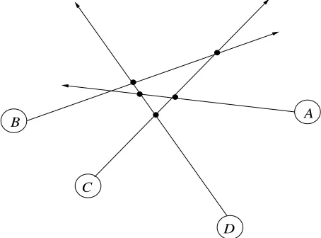
[image:7.612.185.412.23.191.2]A
Figure 1. Initial positions and velocities of four particles. The bullets indicate the positions where the particles are potentially scattered. The shown configuration is not very likely and consequentially the collision trees are quite complex. Note that not every subset of intersection points of the arrows is a set of potential scattering position. For example, it is not possible to add another bullet at the intersection point of the arrows Aand B as it is not possible to assign to each of the six intersections a scattering time which is compatible with the order of the bullets on each ray.
2.2. The concept of trees. The translation of the n-body evolution into scattering statesβ is greatly facilitated by the concept of trees. In the collision tree with root (u, v) we will collect information of collisions and potential collisions up to timet for a particle with initial data u, v.
As an example assume that n = 4 and consider the scenario in fig. 1 where the letters A, B, C, Dare the labels of the four particles, the empty circles are the initial positions and the arrows are the initial velocities. Consequentially the arrow-tips indicate the positions of the particles at timet = 1. To determine whether a certain particle has been scattered before time t = 1 it suffices to analyze the associated collision tree which is constructed as follows: The particle of interest is the root with initial data (u, v). The particles which are potentially scattered by the root are added as leaves, i.e. a particle with initial data (u0, v0) is added, if|u+sv−(u0+sv0)| ≤afor somes ∈[0, t]. This procedure is recursively
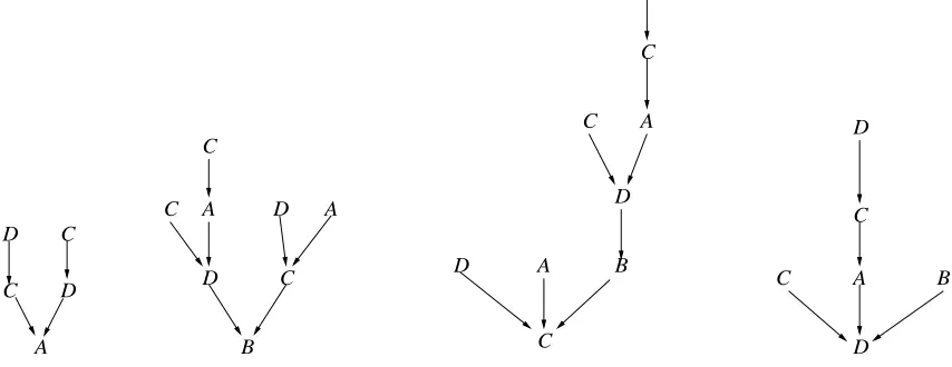
applied to every leaf but we consider only potential scattering events which are upstream, i.e. before the event which is responsible for adding the leaf. The four collision trees associated to the scenario in fig. 1 are shown in fig. 2. The extraction of the collision trees amounts to a significant reduction of the complexity of the problem. In general, the number of potential scattering events (bullets) is proportional to N but thanks to the Boltzmann-Grad-scaling (1) the number of nodes in the individual trees is a Poissonian random number with an intensity which is asymptotically independent of N and grows exponentially with t, see Lemma 12.
We convert now the example into a general concept.
Definition 7. Let N={1,2, . . .}. The height of a node (or multi-index)l ∈Ni is defined
by |l| := i, the child node of l ∈ Ni is ¯l = (l
1, . . . , li−1). Let F = ∪∞i=1Ni be the set of multi-indices. We say that m⊂ F is a tree skeleton with α roots (m∈ Tα), if
(1) #m <∞,
(2) m∩N={1, . . . , α},
(3) ¯l∈m for all l∈m\N,
D A
D A
C
B D C A
C D
D
B C
C
C D
C D
D C
B A
A D A C
[image:8.612.85.512.33.198.2]C
Figure 2. Collision trees of the four particles with initial positions and collision structure given in fig. 1. At time t = 1 particles C and D have been scattered, particles A and B have not. Note that the labels of the particles which generate the potential scattering events are only included in the picture in order to illustrate the translation of fig. 1 into collision trees. The scattering state of the particle at the root is completely determined by the tree structure, the labels of the tree nodes are irrelevant. For example, the tree of particleB does not contain enough information to decide whether particle A is scattered.
(4) l−1∈m for all l ∈m such that l 6= (∗, . . . ,∗,1),
where l−1 = l−(0, . . . ,0,1). We say that a tree m has at most height k (m ∈ T α k ) if
m∩Nk+1 =∅.
Let Y ={(u, v, s, ν)∈Td×Rd×[0,∞)×Sd−1}be the space of initial values and collision parameters. The set of collision trees is given by
Tα
(Y) =
(m, φ)
m∈ T
α
, φ:m→Y with the property sl ∈[sl−1, s¯l]
and νl = 1a(u¯l−ul+sl(v¯l−vl)) for all l ∈m\N
,
where s(∗,...∗,0) = 0. For each skeleton m∈ Tα we define the set
(19) E(m) ={( ˜m, φ)∈ Tα(Y)|m˜ =m},
which contains all trees with skeleton m.
For example, {(1),(1,1),(1,2),(1,3),(1,1,1),(1,1,2)} ∈ T3, but {(1),(2,1)} is not a tree
skeleton. The assumption sl ∈ [sl−1, s¯l] implies that for all nontrivial permutations π ∈
S#m \Id (Sn is the set of permutations of n symbols) and all trees Φ = (m, φ)∈ T1(Y)
the permuted tree Φπ = (m, φπ) withφπ
l =φπ(l) is not a tree in the sense of Definition 7.
The values νl for l ∈ {1, . . . , α} have no relevance. To circumvent this problem we fix a
point ν∗ ∈(Sd−1)α, define
Tα∗(Y) ={Φ∈ Tα(Y)|ν
l=νl∗ ∀l ∈m∩N}.
and will in future denoteTα∗(Y) by Tα(Y).
It is clear from the definition that for each tree m ∈ T there exists a function r : m → N∪ {0}which counts the number of direct successors, i.e.
We will observe the particles 1, . . . , αin the sense that we are interested in evaluating the probability measure on Tα(Y) which is the joint distribution of the trees generated by α
root-particles. In our entire analysis α will be a small natural number, independent ofN ora.
Remark 8. Graph theoretical description of collisions in a hard-sphere gas can lead to many different graphs, which are not necessarily trees. The advantage of our definition is that this graph will always be a tree. Particles might appear several times in a tree, as in fig. 2. This will not destroy the tree structure, as these are due to different collision events. Multiple collisions, which are well-defined in our setting, can lead to identical branches within the tree, but the definition T will discriminate between these and the graph of collisions is still a tree. The only slight abuse of graph-theoretical language is that elements in Tα with α >1 are still called trees and not “forests”.
The scattering state β:m → {0,1}is determined uniquely by the skeleton, i.e. the labels of the particles are immaterial, but the actual computation is not completely trivial. The most important aspect of the computation of β is that the scattering information flows from the leaves to the root, i.e. the scattering state of a node is completely determined by the state of the nodes above, the nodes below are irrelevant.
We will construct now two families of probability measures Pt,k,Pˆt,k∈P M(Tα(Y)).The
empirical distribution ˆPt,k is induced by the many-body dynamics and will be constructed
recursively in Section 2.4. The mean-field distributionPt,k is given by an explicit formula
(20). The link between Pt,k and ˆPt,k is provided by the set of good trees G(a) ⊂ Tα(Y)
(Definition 15) which has the properties that restriction of ˆPt,k onG(a)∩ Tα(Y) converges
toPt,k and Pt,k(G(a)) goes to 1 as a tends to 0 (Proposition 17).
This is the crucial step which eventually yields the justification of the mean-field theory. In other words, the main task consists in analyzing the mean-field measure Pt,k, the
empirical distribution ˆPt,k enters only when we prove thatPt,k is consistent with ˆPt,k.
2.3. The mean-field distribution Pt,k. We construct now the mean-field distribution
of trees Pt,k ∈ P M(Tα(Y)). Let Ω⊂ Tα(Y) and t ∈ [0,∞). The mean field probability
that the observed tree is in Ω is given by
Pt,k(Ω) = X
m∈Tα k
Z
Ω∩E(m)
e−P
j<kΓj(Φ)dλm(φ)
(20)
where
Γj(Φ) = X
l∈m,|l|=j
γl(Φ),
γl(Φ) = Z sl
0
L[f0](vl) ds0 =slL[f0](vl)≥0 is the collision rate of particle l,
λm(φ) = α Y
i=1
[µ(zi)⊗δ(si−t)]⊗ Y
l∈m\N
((vl−v¯l)·νl)+χ[sl−1,s¯l](sl) df0(vl) dνldsl
, (21)
µ(u, v) =1Td(u)⊗f0(v).
Remark 9. (1) Note that the positions ul are completely determined by (ul, vl)l∈m∩N
and (vl, sl, νl)l∈m\N. Since we have assumed that (νl)l∈m∩N is fixed, the value of
Pt,k(Ω) is well-defined.
(2) It is noteworthy that the measures Pt,k depend on time only via the parameter t.
In other words, time plays the role of a parameter which propagates through the tree and qualifies the local branching structure.
(3) For some event Ω ⊂ Tk(Y) the probability Pt,k0(Ω) is independent of k0 if k0 > k.
Equivalently, Pt,k1(Ω ∩ E(m)) = Pt,k2(Ω ∩ E(m)), if the height of m is strictly
smaller thanmin{k1, k2}.
We can simplify the measure Pt,k by integrating over the collision parameters νl ∈Sd−1,
l ∈m. Let ˆY =Rd ×[0,∞) be the reduced set of collision data. For every Ω ⊂ Tα( ˆY)
we find that when still denoting the collision data as φ
¯
Pt,k(Ω) = X
m∈Tα k
Z
Ω∩E(m)
d¯λm(φ)e−P
j<kΓj(Φ)
(22)
with
¯
λm(φ) = α Y
i=1
[f0(vi)⊗δ(si−t)]⊗ Y
l∈m\N
κk|vl−v¯l|χ[sl−1,s¯l](sl) df0(vl) dsl
.
The measures Pt,k have the remarkable property that the expectation of certain random
variables can be computed efficiently.
Definition 10. A random variable x : T1 → R is said to be recursive if there exists a family of functions hb :Rb → R, b ∈N, which are invariant under permutations of the b
components in Rb, such that for all m∈ T the equation
x(m) =hr1(x(m
(1)), . . . , x(m(r1)))
holds, where
m(j) ={(1, l
3, . . . , l|l|)|l ∈m such that l2 =j} ∈ T is the j-th subtree of m.
In the same way one can define vector values recursive random variables x : Tα → Rα.
Examples of recursive random variables which are relevant for our purposes are
x#(m) = #m (number of nodes), xβ(m) =β
1(m) (scattering state of the root).
It is easy to see that if m∈ T1
x#(m) = 1 +
r1
X
j=1
x#(mj),
xβ(m) = r1
Y
j=1
(1−xβ(m
j)) with the convention
0
Y
j=1
(1−xβ(m
j)) = 1,
hence the functions hb are given by
h#b (x1, . . . , xb) = 1 + b X
j=1
xj,
hβb(x1, . . . , xb) = b Y
j=1
(1−xj)
which are clearly invariant under permutations of x1, . . . , xb. Similar expressions are also
valid form∈ Tα withα >1. The expectation of recursive random variables with respect
Lemma 11. Let α = 1 and x be a recursive random variable with recurrence functions
hb. Then
Z
d ¯Pt,k(Φ)x(m)
(23)
=
Z
df0(v)e−Γ1
∞ X r=0 Z t 0 ds1 Z
d ¯Ps1,k−1(Φ1)κd|v−v1|
Z t
s1 ds2
Z
d ¯Ps2,k−1(Φ2)κd|v−v2|
. . .
Z t
sr−1 dsr
Z
d ¯Psr,k−1(Φr)κd|v−vr|hr(x(m1), . . . , x(mr))
=
Z
df0(v)e−Γ1
∞ X r=0 1 r! Z t 0 ds1 Z
d ¯Ps1,k−1(Φ1)κd|v−v1|
Z t
0
ds2
Z
d ¯Ps2,k−1(Φ2)κd|v−v2|
. . .
Z t
0
dsr Z
d ¯Psr,k−1(Φr)κd|v−vr|hr(x(m1), . . . , x(mr))
where Γ1 =κd R
df0(v0)|v−v0|.
An analogous formula holds if α >1.
Proof. For each Φ∈ T( ˆY) we define nonnegative Radon measures ¯λl∈M+(Rd×[0,∞))
by
(24) λ¯l(v, s) = f0(v)|v¯l−v|χ[sl−1,s¯l](s).
With this notation we find the following formula for the measure ¯λm.
¯
λm(φ) =f0(v1)
Y
l∈m\N
¯ λl(φl).
Let now m∈ T1. The definition of P
t,k yields
Z
E(m)
d ¯Pt,k(m)x(m) = Z
E(m)
e−Pj<kΓj(Φ)df 0(v1)
r1
Y
i=1
d¯λ1i(φ1i) Y
l∈m\(N∪N2)
l2=i
d¯λl(φl)
x(m).
We use now the assumption that x is recursive and find
Z
E(m)
d ¯Pt,k(m)x(m)
=
Z
df0(v)e−Γ1
b Y i=1 Z
E(mi)
e−Pj<kΓ
(i)
j (Φ) Y
l∈mj\N
d¯λl(φl)
h(x(m(1)), . . . , x(m(j))),
where Γ(ji)(Φ) =
P
l∈m,|l|=j,l2=i
γl(φ). A simple rearrangement yields that
X
m∈T
Z
E(m)
d ¯Pt,k(Φ)x(m) = Z
df0(v)e−Γ1
∞ X r=0 Z t 0 ds1 Z
d ¯Ps1,k−1(Φ1)κd|v−v1|
. . .
Z t
sr−1 dsr
Z
d ¯Psr,k−1(Φr)κd|v−vr|hr(x(m1), . . . , x(mr)).
This demonstrates the first part of (23), to show the second part we observe that
{(s1, . . . , sr)∈[0, t]r |sj 6=si for i6=j}
= [
π∈Sr
{(s1, . . . , sr)∈[0, t]r |sπ(1) < sπ(2) < . . . < sπ(r)},
where Sr denotes the symmetric group onr elements, such that the union is disjoint. As
the set, where sj =si for somei6=j is of measure zero with respect to Lebesgue measure
ds1. . .dsr, we obtain Z
[0,t]r
g(s1, . . . , sr) ds1. . .dsr = X
π∈Sr
Z
0≤sπ(1)<sπ(2)<...<sπ(r)≤t
g(s1, . . . , sr) ds1. . .dsr
for any g ∈L1([0, t]r). Now we define
g(s1, . . . , sr) = Z
d ¯Ps1,k−1(Φ1)κd|v−v1|. . .
Z
d ¯Psr,k−1(Φr)κd|v−vr|h(x(m1), . . . x(mr)).
We now observe, that ¯
Ps1,k−1(Φ1)κd|v−v1|. . .P¯sr,k−1(Φr)κd|v−vr|
(25)
= ¯Psπ(1),k−1(Φπ(1))κd|v−vπ(1)|. . .P¯sπ(r),k−1(Φπ(r))κd|v−vπ(r)|
for all permutations π ∈ Sr. Next using (25) and the invariance h under permutations,
we obtain
Z
0≤s1<s2<...<sr≤t
Z
d ¯Ps1,k−1(Φ1)κd|v−v1|
. . .
Z
d ¯Psr,k−1(Φr)κd|v−vr|h(x(m1), . . . x(mr)) ds1. . .dsr
=
Z
0≤sπ(1)<sπ(2)<...<sπ(r)≤t
Z
d ¯Psπ(1),k−1(Φπ(1))κd|v−vπ(1)|
. . .
Z
d ¯Psπ(r),k−1(Φπ(r))κd|v−vr|h(x(mπ(1)), . . . x(mπ(r))) ds1. . .dsr.
As there are r! different permutations in Sr we finally obtain Z
0≤s1<s2<...<sr≤t
Z
d ¯Ps1,k−1(Φ1)κd|v−v1|
. . .
Z
d ¯Psr,k−1(Φr)κd|v−vr|h(x(m1), . . . x(mr)) ds1. . .dsr
=1 r!
Z
[0,t]r
Z
d ¯Ps1,k−1(Φ1)κd|v −v1|
. . .
Z
d ¯Psr,k−1(Φr)κd|v−vr|h(x(m1), . . . x(mr)) ds1. . .dsr.
Summing overr and m completes the proof of (23).
As an application of Lemma 11 we obtain an explicit bound on the expected number of nodes in trees.
Lemma 12. For a tree m ∈ Tα the number of non-root nodes is given by R(m) = P
r∈mrl = #m−α. The expected value of R satisfies the estimate uniformly in k
(26) E(R)≤Kini
α X
l=1
exp(κdKiniti),
with Kini =
R
Rddf0(v) (1 +|v|)
2 as in (3).
Proof. We will only give a proof of (26) in the case α = 1, the general case follows by linearity of the expectation. Let Ft,k(v) = E(R | v1 =v) be the conditional expectation
of R if we know that velocity of the root is v and that the tree is inT1
k. Clearly E(R)≤
supk∈N
R
Rddf0(v)Ft,k(v). The self-similarity relation (23) implies with x(m) =R(m) and
hr(R(m1), . . . , R(mr)) = r+Pri=1R(mi) and γ1 = L[f0](v1)t = κdt R
Rddf0(v0)|v1 −v0|
that
Ft,k(v)
=e−γ1 ∞
X
r=1 1
r!
Z t
0
ds1
Z
d ¯Ps1,k−1(m1)κd|v−v1|
. . .
Z t
0
dsr Z
d ¯Psr,k−1(mr)κd|v−vr| r+
r X
i=1
R(mi) !
=e−γ1 ∞
X
r=1
r(−γ1)
r
r! + γr−1
1
r!
r X
i=1
Z t
0
dsiκd Z
Rd
df0(v(
i)
1 )|v−v (i)
1 |Fsi,k−1(v (i) 1 )
!
=γ1+
Z t
0
ds κd Z
Rd
df0(v0)|v1−v0|Fs,k−1(v0),
where we used the product structure of the integrals. We define now the norm kFk1 :=
supv∈Rd
F(v)
1+|v| and the integral operator Af0 by
(Af0F)(v) =κd
Z
Rd
df0(v0)|v−v0|F(v0),
so that
(27) Ft,k =tγ +
Z t
0
ds AfFs,k−1.
We find the estimates
kAf0Fk1 ≤sup
v
κdkFk1
1 +|v|
Z
Rd
df0(v0)|v−v0|(1 +|v0|)≤KkFk1,
and
kγk1 = sup
v
κd Z
Rd
df0(v0)|v−v
0|
1+|v| ≤κd
Z
Rd
df0(v0) (1 +|v0|)≤κdKini.
Furthermore Ft,k(v) is monotone in k, as Pt,k assigns the probability of trees of height
greater than k + 1 to trees of height k, reducing the number of expected nodes. Hence equation (27) implies that
kFt,kk1 ≤κdK
t+
Z t
0
dskFs,kk1
.
Gronwall’s inequality together with the previous estimate implies that
kFt,kk1 ≤eκdKinit,
where we used that F0 ≡0. Since
Ek(R) =
Z
Rd
f0(v)Ft,k(v)≤ kFtk1
Z
Rd
df0(v) (1 +|v|)≤KeκdKinit
this implies (26) for α= 1 and the proof of the lemma is finished.
We now turn our attention to the determination of the scattering state of the particle at the root of the tree. For a tree m ∈ Tα the scattering state β : m → {0,1} is defined
recursively by βl = Q
l0∈m,l¯0=l(1−βl0). This definition rephrases the original definition of
the scattering state in (16), adapting it to the tree structure. It is more convenient in our analysis than the ad-hoc definition, which required already some work to show existence, see Lemma 6.
We define the single-particle density gt,k(·)∈M+(Rd) via
Z
A
dgt,k(v) =Pt,k(β1 = 1 andv1 ∈A),
for all open A ⊂ Rd. The density g
t,k is closely related to the root marginal of Pt,k
and provides the link between the Boltzmann equation (5) and the mean-field theory distribution of the trees Pt,k. Due to the simplicity of the distribution Pt,k it is possible
to characterize the root-marginal ofPt,k explicitly.
Proposition 13. Let α∈N, σ :Tα
1 → {0,1}, A⊂Rd, t∈[0,∞) andk∈N∪ {0}. Then the equation
Pt,k+1(vl ∈A and βl =σl for all l∈ {1. . . α})
=
α Y
l=1
Z
A
dv [(1−σl) (df0(v)−dft,k(v)) +σldft,k(v)]
(28)
holds, where ft,k is the solution of system (15).
This formula shows that in particular gt,k =ft,k−1.
Proof. The proposition is proven using induction over k, the case k= 0 is just the defini-tion.
In the induction step it is demonstrated thatPt,k+1 satisfies formula (28) ifPt,kdoes. Since
the collision parameters ν are irrelevant we can integrate them out and work with the simplified version (22) of the measure Pt,k instead of (20). We define the set of scattering
states that are compatible with σ,
A(σ) =
(m, σ0)
m∈ Tα
2 , σ0 :m→ {0,1}such that
Y
l0∈m,¯l0=l
(1−σ0l0) =σl ∀l
, (29)
with the standard convention Q0j=1aj = 1 for empty products. The induction assumption
and equation (23) implies that
Pt,k+1(vl ∈A and βl =σl for all l = 1, . . . , α)
= X
(m,σ0)∈A(σ) Z
v∈A Y
l∈m∩N
e−γl
rl! df0(vl)
Y
l0∈m
¯
l0=l
(1−σl00) Z sl
0
ds
Z
v0∈Rd
κd|vl−v0|(df0(v0)−dfs,k−1(v0))
+σl00 Z sl
0
ds
Z
v0∈Rd
dfs,k−1(v0)κd|vl−v0|
=
Z
v∈A
X
(m,σ0)∈A(σ) α Y
l=1
[df0(vl)Ik(σ0, v, l)]
where
Ik(σ0, v, l)
=e−γl
rl!
Y
l0∈m,l¯0=l
(1−σ0l0) Z tl
0
ds
Z
v0∈Rd
κd|vl−v0|(df0(v0)−dfs,k−1(v0))
+σ0l0 Z tl
0
ds
Z
v0∈Rd
dfs,k−1(v0)κd|vl−v0|
=e−γl
rl!
Y
l0∈m,l¯0=l
(1−σ0l0)
γl− Z tl
0
ds L[fs,k−1](vl)
+σl00 Z tl
0
ds L[fs,k−1](vl)
.
Note that A(σ) = Qαl=1A(σl) if we identify single trees with α roots and α trees with
single roots. The algebraic identity Pi∈IJ
Q
j∈Ja(ij, j) = Q
j∈J P
i∈Ia(i, j), where I and
J are finite sets and a : I ×J → R is a function, implies that P
σ0∈A(σ) α Q
l=1
Ik(σ0, v, l) =
α Q
l=1
P
σ0∈A(σl)
Ik(σ0, v,1). This yields that
Pt,k+1(vl ∈A and βl=σl ∀l = 1. . . α) = α Y
l=1
Z
v∈A
df0(v) [(1−σl)Jk(0, v) +σlJk(1, v)],
(30)
withJk(σ, v) = P
σ0∈A(σ)Ik(σ0, v,1). Since by definitionA(1) ={(1),(1,(0)),(1,(0,0)). . .},
this shows that
Jk(1, v) =
∞
X
j=0
e−γ
j!
γ−
Z s
0
ds0L[f
s0,k−1](v) j
=e−Rs
0ds0L[fs0,k−1](v), (31)
with γ =sL[f0](v). Clearly
R
Adf0(v)Jk(0, v) + R
Adf0(v)Jk(1, v) = R
Adf0(v) and
there-fore
Z
v∈A
df0(v)Jk(0, v) = Z
v∈A
df0(v) (1−Jk(1, v)) = Z
v∈A
df0(v)
1−e−R0sds0L[fs0,k−1]
. (32)
Plugging the formulas (31) and (32) into equation (30) yields that Pt,k+1(vl ∈A and βl =σ ∀l= 1, . . . , α)
=
α Y
l=1
Z
v∈A h
(1−σl) df0(v)
1−e−R0tlds L[fs,k−1]
+σldf0(v)e−
Rtl
0 ds L[fs,k−1]
i (15) = α Y l=1 Z
v∈A
[(1−σl) (df0(v)−dftl,k(v)) +σldftl,k(v)]
and formula (28) has been established.
2.4. The empirical distribution Pˆt,k. We return now to the hierarchy of many body
evolutions described in Section 2.1. The initial values of the particles form a random set ω ⊂Td×Rd and it is assumed that the law ofω is the Poisson point process with density
N µ, where µ=1Td⊗f0 ∈P M(Td×Rd). Hence, the size n = #ω is Poissonian random
variable with intensityN. As explained in Section 2.2, the family of probability measures ˆ
Pt,k ∈ P M(T(Y)) is the empirical distribution of the tree Φ which is generated by the
many-body evolution and has a randomly chosen (tagged) particle as its root. This tree
is only well defined ifn > 0, i.e. ω is non-empty. For this reason we define Pt,k(Ω) as the
conditional probability that the tree is contained in the set Ω, given that n = #ω >0. A particularly simple method of sampling from this conditional distribution consists in drawing a realization of ω according to the unconditioned Poisson point process, and an independent random variable z ∈ Td ×Rd with law µ(z) = 1
Td(u)⊗f0(v) which is the
initial value of the tagged particle. It can be checked without difficulty that the joint distribution of ω and z is the previously defined conditional distribution.
The trees generated by this procedure are denoted by Φ(t, k) = (m(t, k), φ) ∈ Tk(Y),
where m(t, k) ∈ Tk is the skeleton and φ : m(t, k) → Y specifies the initial values, the
collision times and the impact parameters. The measures ˆPt,k are the image measure of
Probppp induced by the many-particle flows so that for each Ω⊂ T(Y) we obtain
(33) Pˆt,k(Ω) := Probppp((m(t, k), φ)∈Ω).
The tree measures ˆPk are derived from Probppp, but Probppp cannot be derived from ˆPt,k.
By construction, for fixed ω the skeleton m is monotonously increasing in t and k, and for fixed l ∈ m the data φl does not depend on t or k. This is equivalent to saying that
the j-marginal of ˆPt,k (trees of hight j ≤k) is given by ˆPt,j, i.e.
ˆ
Pt,k m(t, k)∩(∪ji=1N
i),(φ l)|l|≤j
∈Ω= ˆPt,j((m(t, j),(φl)|l|≤j)∈Ω)
(34)
for all Ω⊂ Tj(Y), k≥j.
We will use formula (34) to construct an alternative characterization of ˆPt,k which reflects
the iterative process that underlies the definition of m(t, k). Using this alternative char-acterization one can easily establish total-variation bounds forPt,k−Pˆt,k. Since the time
t is arbitrary but fixed we will often write ˆPk instead of ˆPt,k.
Let (m0, φ0)∈ T
k−1(Y) and let ˆPk(· |(m0, φ0))∈ P M(Tk(Y)) be the conditional
distribu-tion of ˆPk in the sense that
ˆ
Pk(Ω|(m0, φ0)) := ˆPk
(m(k), φ)∈Ω|m∩Nj =m0∩Nj for all j ∈ {1. . . k−1}
and φl =φ0l for all l∈m such that|l|< k
.
Formula (34), which characterizes the j-marginals of ˆPt,k, yields the following recurrence
relation for ˆPk:
(35) Pˆk(Ω) =
Z
Tk−1(Y)
d ˆPk−1(Φ0) ˆPk(Ω|Φ0).
Repeating this step k−1 times we obtain the following iterative representation of ˆPk:
ˆ
Pk(Ω) = Z
T1(Y)
dP1(Φ1)
Z
T2(Y)
d ˆP2(Φ2|Φ1). . .
Z
Tk−1(Y)
d ˆPk−1(Φk−1|Φk−2) ˆPk(Ω|Φk−1),
(36)
where
(37) P1(z1. . . zα) = α Y
l=1
µ(zl)∈P M (Td×Rd)α
is the distribution of α initial values.
2.5. Convergence of Pˆk to Pk. Having constructed an iterative characterization of ˆPk
we will now show that it is very similar to the mean field measure Pk in a precise way.
The key is to identify the mechanisms by which the two probability distributions fail to be equal. In this part of the paper we will work with the phase-space representation of the trees: zl = (ul, vl)∈Td×Rd.
Remark 14. There are only two reasons why Pˆk fails to coincide with Pk in the limit
a→0:
(1) The cylinders which are covered by the paths of the particles might contain self-intersections due to the periodic boundary conditions: v−v0 ∈R(t, a) with
(38) R(t, a) =v ∈Rd | min{|s v−ξ| |s∈[0, t], ξ∈Zd\ {0}} ≤ a .
(2) Nodes might have more than one child, i.e. the map z : m → Td ×Rd might be
not injective.
The setR(t, a), which can easily seen to be nonempty, is relevant due to periodic boundary conditions, which will lead to self-intersections of the cylinders. This happens, if v −vj
is sufficiently close to a velocity v∗, where the components of v∗
1, . . . , vd∗ are rationally
dependent, i.e. η·v∗ ∈Z with η ∈Zd, but only if |η| ≤ t. The effect is not present in a
setting where (u, v)∈Rd×Rd.
The second effect is caused by the notorious recollisions. These dependencies disappear as the diameter a tends to zero.
We stipulate now a strict order of the set of nodes m:
l < l0 if either |l|<|l0| or (|l|=|l0| and ¯l <l¯0) or (¯l = ¯l0 and l
|l|< l0|l|)
(39)
This order is induced by the link between the collision time and the indices l ∈ m in Definition 7.
Motivated by Remark 14 we define the set of “good” trees.
Definition 15. For each a0 > 0 the set of “good” trees G(a0) ⊂ T(Y) consists of those trees (m, φ)∈ T(Y) with the property that for all 0< a≤a0 and all l∈m
vl−v¯l ∈R d \
R(t, a) (all parent-child-pairs are non-resonant),
(40)
zl6∈ ∪l0<l l06=¯l
Cl0 (no node has more than one child),
(41)
where we associate to each node l ∈m the set of colliding initial values
Cl =
z0 ∈Td×Rd
s0min∈[0,sl]|dist(zl, z
0, s0)| ≤a
,
and dist as in (8) ignores overlap in the initial data.
Note that G(a0) ⊂ T(Y) is a family of sets which decreases with a0. An elementary
calculation yields that for all v0 ∈Rd\(v
l+R(t))
(42) NHd−1 C
l∩(Td × {v0})
=κd|vl−v0|sl.
The significance of G(a0) is given by the following results
lim
a0→0 inf
k Pk(G(a0)) = 1,
(43)
lim
a→0supk
Pˆk(Ω)−Pk(Ω)
= 0 for all Ω⊂ G(a0) if a0 is fixed,
(44)
which are proven in Proposition 17. For the proof we need a more explicit characterization of the distributions ˆPk(· |Φk−1) and ˆPk(·)
As an intermediate step we recall a formula which yields the probability of certain complex events with respect to Poisson-point processes. Let A ⊂ ∪∞
n=0(Td ×Rd)n be a symmetric
set, i.e. z ∈ A∩ (Td × Rd)n if and only if (z
π(1), . . . , zπ(n)) ∈ A∩ (Td ×Rd)n for all
permutations π ∈ Sn, where Sn is the symmetric group. We use the convention that
(Td ×Rd)0 is a single point. For each realization ω ⊂ Td ×Rd of the point process we
chose an arbitrary enumeration of the elements of ω such that ω ={z1, . . . , zn}. We say
that ω ∈ A if (z1, . . . , zn) ∈ A; the choice of the enumeration is irrelevant since A is
symmetric. It can be checked that if ω is a realization of the Poisson-point process with intensity µ∈M+(Td×Rd), then
(45) Probppp(ω∈A) =e−µ(
Td×Rd) ∞
X
n=0
1 n!
Z
A∩(Td×Rd)n
dµ(z1). . .dµ(zn),
where the value of integral forn= 0 is 1 if (Td×Rd)0 ⊂Aand 0 else. By the definition of
Poisson-point processes each set C ⊂ Td×Rd defines a projection denoted by C ∩ω. We
recall the following fundamental independence-principle of Poisson-point processes which asserts that even if we have obtained a certain amount of information over a realizationω of a Poisson-point process it is still possible to use a suitably modified version of formula (45).
Lemma 16. Let the random setω ⊂Td×Rd be distributed according to a Poisson point-process with density µ, C¯,C ⊂ Td ×Rd and A ⊂ ∪∞r=0(C \C¯)r be symmetric. Then we obtain the following formula for the conditional probability of the event A:
Probppp ω∩ C ∈ A
ω∩C¯=∅= exp −µ(C \C¯)
∞
X
r=0
1 r!
Z
A∩Cr
dµr(z),
(46)
where µr =µ⊗. . .⊗µ
| {z }
rterms
Proof. See section 4.
To apply Lemma 16 we have to work with the phase space representation of trees. Owing to the decomposition Ω = ˙∪m∈TE(m)∩Ω we can assume that Ω⊂ E(m) for some m∈ T.
Due to this simplification we can drop the sum in equation (46) since only one term is nontrivial.
Note that for a general tree Φ = (m, φ) ∈ T(Y) the number of nodes #m can be bigger than the number of particles involved in the collisions, i.e. it is possible that the map z : m → Td ×Rd is not injective and zl = zl0 for some pair l, l0 ∈ m, l 6= l0. This
scenario corresponds to a bad tree where one node has two child nodes. For this reason we restrict our attention to sets Ω which are subsets ofG(a). The excluded set has nonzero probability, however we will show that the probability of T(Y)\ G(a) tends with a to 0. By construction for all trees in Ω the mapl 7→zl is injective.
The order defined by (39) induces a representation of the events Ω⊂ T(Y) in phase-space coordinates:
A(Ω) ⊂(Td ×Rd)#m.
In the same spirit one obtains a one-to-one correspondence between the the initial values of particles associated with the tree-nodes at height k and subsets of (Td ×Rd)#m∩Nk
:
Zk= (zl)|l|=k∈(Td×Rd)#m∩
Nk
. We will also need the conditional events
Ak(Ω,Φ) = n
Zk∈(Td×Rd)#m∩
Nk
|(Zk,Φ) ∈Ω o
,
where Φ ∈ Tk−1(Y) and (Zk,Φ) ∈ Tk(Y) is the tree obtained by attaching the leaves Zk
to the topmost nodes of Φ.
Recall that the density of the Poisson-point process which generates the initial positions of the particles is given by N µ where
Z
dµ(z)ϕ(z) =
Z
Rd
df0(v)
Z
Td
du ϕ(u, v)
for every testfunction ϕ∈Cc(Td ×Rd).
Before applying Lemma 16 we have to specify the sets C and ¯C. Fix a0 > 0 and let
Φ ∈ T(Y)∩ G(a0). We are interested in the distribution of those trees which coincide
with Φ up to level k. Clearly, the initial positions of the particles at height k + 1 are contained in the set
Ck(Φ) := [
l∈mk∩Nk
Cl(φ)⊂Td ×Rd,
with Φ = (m, φ). In order to apply formula (46) we have to identify the conditioning of the distribution ω∩ Ck(Φ). Define the collection of cylinders
¯
Ck(Φ) := [
|l|<k
Cl(φ)⊂Td ×Rd
which contains those initial values that would affect the lower nodes. By construction the information on the point processωthat we have accumulated so far is given byω∩C¯k(Φ) =
{zl | |l| ≤ k}. Furthermore, since Φ ∈ G(a0) we have that ω∩ Ck(Φ)∩C¯k(Φ) = ∅. This
implies that for each Ω⊂ T(Y)∩ G(a0) and Φ∈ Tk(Y)∩ G(a0) that
ˆ
Pk+1(Ω|Φ) = Probppp(Ck(Φ)∩ω∈sym(Ak(Ω,Φ))| Ck(Φ)∩C¯k(Φ)∩ω =∅).
where sym(A) is the symmetrization of the set A, i.e. (z1, . . . , zn) ∈ sym(A) if there
exists a permutation π ∈ Sn such that (zπ(1), . . . , zπ(n)) ∈ A; in particular A ⊂ sym(A).
This is the crucial step where the complicated dependency on the past of the many-body evolution is reduced to a simple conditional expectation of the Poisson point process. Since A(Ω,Φ)∩C¯k(Φ)×. . .×C¯k(Φ)
| {z }
rterms
=∅ for each r we can use formula (46) and deduce
that
Pk+1(Ω|Φ) =e− ˆ Γk(Φ)1
r!
Z
sym(Ak+1(Ω,Φ))
dµr(Zk+1)
where
(47) Γˆk(Φ) =µ( ˆCk(Φ))
and ˆC(k) = Ck(Φ) \ C¯k(Φ). Recall the convention that the value of the integral over
(Td×Rd)0 is 1.
Since each permutation of the labels l ∈m destroys the tree structure we obtain that if zπ ∈ A and z ∈ A, then necessarily π is the identity transformation, i.e. zπ = z. This
implies that if we replace in the above formula sym(A) by the non-symmetric set A we have to drop the term 1
r!.
Pk+1(Ω|Φ) =e− ˆ Γk(Φ)
Z
Ak+1(Ω,Φ)
dµr(Zk+1).
(48)
Plugging the expression (48) for the conditional expectation ˆPk+1(· |Φ) into equation (36)
yields that
ˆ
Pk(Ω) = Z
(Td×Rd)α
dP1(φ1(Z1))e− ˆ
Γ1(Φ1(Z1))
Z
(Td×Rd)r2
µr2(Φ
2(Z2))
. . . e−ˆΓk−1(Φk−1(Z1...Zk−1))
Z
Ak(Ω,Φk−1(Z1...Zk−1))
dµrk(Z
k)
= X
m∈Tk
Z
A(Ω)
dµ#m(z)e−P
j<kΓjˆ (Φ(z)).
(49)
The intermediate step in the computation above relies on the additional assumption that m∈ Tk\Tk−1. In general we have to be more careful concerning the domains of integration,
but the the final formula is unaffected.
We return now to the collision representation of the trees. This means that the variables (zl)l∈m are replaced by (u1, v1)×(sl, νl, vl)l∈m\N if α = 1 and analogously if α > 1. The
determinant of the derivative of this transformation is given by
detDΦz(Φ) =
Y
l∈m\N
ad−1[νl·(vl−v¯l)]+.
Thus changing coordinates in the integrals we obtain that for each m ∈ T
Z
A(Ω)
e−Pj<kΓj(Φ(ˆ z))dµ#m(z)
=
Z
Ω
dP1(z1. . . zα)e−
P
j<kΓjˆ (Φ) Y
l∈m\N
Ndf0(vl) dνldslχ[0,s¯l](sl)a
d−1[(v
l−v¯l)·νl]+
(1)
=
Z
Ω
dP1(z1. . . zα)e−
P
j<kΓjˆ (Φ) Y
l∈m\N
df0(vl) dνldslχ[0,s¯l](sl) [(vl−v¯l)·νl)]+
=
Z
Ω
dλm(φ)e−Pj<kΓjˆ (Φ),
Thus we have shown that for all Ω⊂ G(a)
(50) Pˆk(Ω) =
X
m∈Tk
Z
Ω∩E(m)
e−P
j<kΓjˆ (Φ)dλm(φ).
and
(51) Pk(Ω) = ˆPk(Ω) +ek(Ω),
where the error has the form
ek(Ω) = X
m∈Tk
Z
Ω∩E(m)
dλm(φ)e−P
j<kΓjˆ (Φ)−e−
P
j<kΓj(Φ)
. (52)
Since ˆΓj(Φ) ≤Γj(Φ) the difference ek(·) is a non-negative measure.
Now we are in a good position to prove that equations (43) and (44) hold.
Proposition 17 (Similarity of ˆPk and Pk). Let G(a) the set of good trees from
Defini-tion 15, and Ω⊂ G(a0). Then equations (43) and (44) hold.
Proof. For technical reasons we decouple the dependency of G and ˆPk on the scaling
parameter a. We will construct a family of sets of trees ˆG(a)⊂ G(a) with the following two properties
lim
a0→0 inf
k Pk
ˆ
G(a0)
= 1, (53)
lim
a0→0 lim
a→0supk
Pˆk
Ω∩Gˆ(a0)
−Pk
Ω∩Gˆ(a0)
= 0
(54)
for all Ω ⊂ T(Y). The idea is that the trees in the sets ˆG(a0) have additional good
properties which are controlled by a0. It is quite clear that for our choice of ˆG(a0) (see
(56)) equation (54) holds even for fixed a0 but without the limit the proof becomes more
complicated.
We show first that (53) and (54) imply (44): Since ˆPk and Pk are probability measures
equation (53) implies that
(55) lim
a0→0 lim
a→0supk
Pˆk
T(Y)\Gˆ(a0)
−Pk
T(Y)\Gˆ(a0)
= 0.
Let now Ω⊂Gˆ(a0) for somea0 >0 and fix ε >0. Then
lim
a0→0 lim
a→0supk |
ˆ
Pk(Ω)−Pk(Ω)| ≤ lim a0→0
lim
a→0supk
Pˆk
Ω∩Gˆ(a0)
−Pk
Ω∩Gˆ(a0)
+ lim
a0→0 lim
a→0supk
ˆ Pk
Ω\Gˆ(a0)
+ sup
k
Pk
Ω\Gˆ(a0)
(54)
= lim
a0→0 lim
a→0supk
ˆ Pk
Ω\Gˆ(a0)
+ lim
a0→0 sup
k
Pk
Ω\Gˆ(a0)
(55) ≤2 lim
a0→0 sup
k
Pk
T(Y)\Gˆ(a0)
(53)
= 0.
Equation (43) follows directly from (53) since ˆG(a)⊂ G(a).
Letε(a) andV(a) be monotone functions ofasuch that lima→0ε(a) = 0 and lima→0V(a) =
+∞. which will be determined later. We define the set
ˆ
G(a0) =
\
a<a0
(m, φ)∈ G(a)
l,lmin0∈m
l0 6=l
|vl−v¯l| ≥ε(a) and |v| ≤V(a)
(56)
and min
l∈m l0<l,lmin06=¯l
1−
vl−v¯l
|vl−v¯l|·
vl0−v¯l
|vl0−v¯l|
≥ε(a) .
Due to the monontonicity of ε(a) and V(a) the set ˆG(a) is increasing with a.
Before proving (53) and (54) we will first estimate the size of the set R(t, a) and demon-strate that
(57) lim
a→0
Z
R(t,a)
(1 +|v|) df0(v) = 0.
For each ξ∈Zd \ {0} we define the cone
M(ξ, a) =v ∈Rd|(v·ξ)2 ≥(|ξ|2−a2)|v|2 .
Let c(a) := sup{RM(ξ,a)df0(v)|ξ ∈ Zd \ {0}} be an upper bound for the volume of this
cone. Assumption (4) implies that c(a) =o(1) as a → 0. For each v ∈ R(t, a) such that
each velocity v ∈ R(t, a) is an element of one of at most (2tV + 2a)d cones. Thus we
obtain, using (3),
Z
R(t,a)
(1 +|v0|) df0(v0)≤
Z
R(t,a)∩{|v0|≤V}
(1 +|v0|) df0(v0) +
Z
{|v0|>V}
(1 +|v0|) df0(v0)
≤(1 +V)(2tV + 2a)dc(a) +Kini/V,
withKini =
R
Rddf0(v) (1 +|v|)2. So choosing first V large the second term is small. Then
choose a so that the first term is small, which completes the proof of the equation (57).
Proof of equation (53).
First we show that we can restrict ourselves to bounded trees. By Lemma 12, the expected value of the number of nodes #m in a tree m is bounded by Kiniexp(κdKinit). As #m is
a positive function, this implies immediately the estimate
(58) X
#m−α>r
Pk(E(m))< Kriniexp(κdKinit).
This estimate gives us control over the error which arises if we ignore all trees with more than r nodes:
1 = X
m∈T
Pk(E(m)) = X
m∈T
#m−α≤r
Pk(E(m)) + X
m∈T
#m−α>r
Pk(E(m))
≤ X
m∈T
#m−α≤r
Pk(E(m)) + KrinieκdKinit.
(59)
In particular, if r≥ Kini
δ e
κdKinit +α, then
(60) X
m∈T
#m≤r
Pk(E(m))≥1−δ.
Recall the ordering of the tree nodesl ∈mgiven by (39) and that ¯ldenotes the child-node of l∈m\N. Define for eachl ∈m and each Φ∈ T(Y)∩ E(m) the (possibly empty) sets
Gl(Φ, a) = \
a<a0
(s, ν, v)∈[0, s¯l]×Sd−1×Rd
v−v¯l
|v−v¯l|·
vl0−v¯l
|vl0−v¯l|
≥ε(a) for all l0 < l, l0 6= ¯l
and v −v¯l 6∈R(t, a) and (ul(s, ν, v), v)6∈ [
l0<l,l06=¯l
Cl0 and |vl−vl0| ≥ε∀l0 < l
,
Bl(Φ, a) =[0, s¯l]×Sd−1×Rd\Gl(Φ, a),
Bl(a0, a) ={Φ∈ T(Y)∩ E(m)|φl ∈Bl(Φ, a) andφl0 ∈Gl0(Φ, a0) ∀l0 < l}.
Note thatB1(a0, a) =B1(Φ, a). The set Bl contains those trees which have node l as the
first bad node. It is easy to see that Gl(Φ, a) and Bl(Φ, a) are monontone in a and that
E(m) =Gˆ(a)∩ E(m)∪˙l∈mBl(a, a), i.e. the set E(m) can be written as a disjoint union
of good trees and the sets Bl and we obtain that
Pk
ˆ
G(a)= X
m∈T
Pk(E(m))− X
l∈m
Pk(Bl(a, a)) !
.
Another easy consequence is that
(61) X
l∈m
Pk(Bl(a, a))≤Pk(E(m)).
A simple computation shows that for any sequence a0 =a1 ≥. . .≥al =a the estimate
Pk(Bl(a, a))≤ X
l0≤l
Pk(Bl0(al0−1, al0)),
where l0−1 is the predecessor of l0, and thus
1−Pk
ˆ
G(a)≤ X m∈T
#m≤r
X
l∈m,l0≤l
Pk(Bl(al0−1, al0)) +δ
holds. This inequality is far from being optimal but it suffices for our purposes. We will show that for fixed al0−1 each term in the sum can be made small by choosing al0 small
enough. This implies that lima→0Pk
ˆ
G(a) = 0 since we can choose a11 first (or a2 if
α >1) depending on a1 and so on until we reach al which serves as an upper bound for
a.
We define now the functions hm
l,a0,a :E(m)→[0,∞) by hml,a0,a(φ) = e
−Γ(Φ)χ
Bl(a0,a)(φ),
where Γ(Φ) =P|l|<kR df0(v)|v−vl|.Clearly, for fixedl ∈m,a0 >0 the numberhml,a0,a(Φ) is nonnegative, monotonously decreasing in a and bounded from above by the function
gm :E(m)→[0,∞) : gm(φ) :=e−
P
j<kΓj(Φ).
Note thatgm ∈L1(λm), sincegm ≥0 and 1 =Pk(T(Y)) =Pm∈Tk R
E(m)dλ
m(φ)g m(Φ).
Thus, it suffices to show that
(62) lim
a→0λl(Bl(Φ, a)) :=N
Z
Td
du
Z
Rd
dv χBl(Φ,a)∩C¯l(u, v)
for all Φ ∈ E(m)∩ Bl(a0, a). In order to prove estimate (62) we split Bl(Φ, a) into five
sets, the first four are represented in collision coordinates, the last one is expressed in phase-space coordinates.
Bl,1 =
(ν, τ, v)∈Sd−1×[0, s ¯
l]×Rd | |v−vl0| ≤ε for some l0 < l ,
Bl,2 =
n
(ν, τ, v)∈Sd−1×[0, s¯l]×Rd
v−v¯l
|v−v¯l|·
vl0−v¯l
|vl0−v¯l|
≥1−ε for some l0 < l o
,
Bl,3 =
(ν, τ, v)∈Sd−1×[0, s¯l]×Rd |v−v¯l∈R(t, a) ,
Bl,4 =
(ν, τ, v)∈Sd−1×[0, s ¯
l]×Rd | |v|> V(a) ,
Bl,5 =
(u, v)∈ [
l0<l,l06=¯l
Cl0 \
C¯l
|v| ≤V(a) and v−v¯l
|v−v¯l| ·
vl0−v¯l
|vl0−v¯l|
≤1−ε for all l0 < l
.
We will show now that lim
a→0λl(Bl,j(Φ, a)) = 0 for each l ∈ m, j ∈ {1, . . . ,5} and Φ ∈ Bl(a0, a) ifa0 >0 is fixed.
j = 1:
λl(Bl,1) =
X
l0<l l06=¯l
Z
|v−vl0|≤ε
df0(v)
Z
Sd−1 dν
Z s¯l
0
dτ[(v−v¯l)·ν]+
≤X
l0<l Z
|v−vl0|≤ε
df0(v)|v−v¯l|κds¯l.
Thanks to (4) the last expression goes to 0 as ε tends to 0. Since a0 appears
nowhere the convergence is uniform in a0.
j = 2: Let
Mε= [
l0<l,l06=¯l n
v ∈Rd
v−v¯l
|v−v¯l|·
vl0−v¯l
|vl0−v¯l|
>1−ε o
⊂Rd.
As ε tends to 0 the setMε converges to v¯l+R S
l0<l,l06=¯l
(vl0 −v¯l). We obtain that
λl(Bl,2) =
Z
Mε
df0(v)
Z s¯l
0
dτ
Z
Sd−1
dν[ν·(v−v¯l)]+ ≤r
Z
Mε
df0(v)|v−v¯l|κds¯l.
Dominated convergence and assumption (4) imply that
(63) lim
a→0
Z
Mε(a)
df0(v) (1 +|v|)κds¯l = 0,
hence the last expression goes to 0 asε tends to 0. The convergence is uniform in a0.
j = 3:
λl(Bl,3) =N
Z
v¯l+R(t)
df0(v)
Z s¯l
0
dτ
Z
Sd−1
dν[ν·(v −v¯l)]+
≤
Z
vl+R(t)
df0(v)|v−v¯l|κds¯l =
Z
R(t)
df0(v)|v|κds¯l
By equation (57) the last expression converges uniformly ina0 to 0 as a tends to
0. j = 4:
λl(Bl,4) =N
Z
|v|≥V(ε)
df0(v)
Z s¯l
0
dτ
Z
Sd−1
dν[ν·(v−v¯l)]+
≤
Z
|v|≥V(ε)
df0(v)|v−vl|κds¯l
By assumption (3) the last expression converges uniformly ina0 to 0 asεtends to
0.
j = 5: This is the only case where estimates are not uniform and depend on the constantε(a0). We estimate λl(Bl,5) as follows:
λ(Bl,5)≤
X
l0<l l0 6=¯l
N
Z
Rd
df0(v)Hd C¯l(Φ)∩Cl0(Φ)∩(Td× {v}).
To bound Hd C
¯
l(Φ)∩Cl0(Φ)∩(Td× {v})
we define the number c(a0, a, v0) to
be the maximum volume contained within the intersection of two cylinders of diameter a and axes v−v0 and v−v00 if v, v0 and v00 are constrained in a certain
geometrical way:
c(a0, a, v0) = sup
ζ(u0, u00, v, v0, v00, a)
u
0, u00 ∈Td, v, v00 ∈Rd, |v0−v00| ≥ε(a
0)
and |v|,|v00| ≤V(a) and v−v
0
|v−v0|· v00−v0
|v00−v0|
≤1−ε(a0)
,