Design optimization of a new superconducting magnet system for a LAr Neutrino Detector A technical design report performed within the framework of a bachelor assignment as part of the Advanced Technology bachelor programme at the ATLAS magnet group at C

(1)

Design Optimization of a new

Superconducting Magnet System for a LAr

Neutrino Detector

A technical design report performed within the framework of a bachelor assignment as part of the Advanced Technology bachelor programme at the ATLAS magnet group at CERN.

L.Y. van Dijk

Date July 15, 2014

Examination Committee Prof. Dr. Ir. Herman ten Kate

(2)

(3)

Abstract

This report presents a design optimization of a new superconducting magnet system for a liquid Argon neutrino detector. The optimization study is performed within the framework of a bachelor assignment as part of the Advanced Technology bachelor programme at the ATLAS magnet group at CERN.

(4)

1 Introduction

This report presents a design optimization of a new superconducting magnet system for a liquid Argon neutrino detector. The optimization study is performed within the framework of a bachelor assignment as part of the Advanced Technology bachelor programme at the ATLAS magnet group at CERN. In this chapter an introduction is given to particle physics, CERN, neutrino detection, the design requirements and the assignment itself.

1.1 Fundamental Particles

1.1.1 Standard Model

The standard model of particle physics (figure 1.1) is a theory that describes the basic building blocks our universe is made of and the forces that govern their interactions. It was developed during the late 1970s as a collaborative effort of scientists around the world. The model predicted the existence of the bottom quark, the top quark, the tau neutrino and the Higgs boson. Confirmed to exist experimentally in respectively 1977, 1995, 2000 and 2013. Because of its success in explaining a wide variety of experi-mental results, the standard model is sometimes called the ’theory of almost everything’. However, the standard model falls short of being complete since it does not incorporate the full theory of gravitation and neither accounts for the accelerating expansion of the universe.

(7)

1.1.2 CERN and the LHC

One of the largest institutes involved in particle physics is the ’European Council for Nuclear Research’, better known as CERN. It was founded in 1954 by 12 Western European countries and is located on the Franco-Swiss border near Geneva. CERN’s main function is to provide particle accelerators and other infrastructure needed for high-energy physics research. The institute accommodates an accelerator complex which is a succession of machines that accelerate particles to increasingly higher energies. Each machine boosts the energy of a beam of particles, before injecting the beam into the next accelerator in the sequence. The last element in this chain is the Large Hadron Collider (LHC) which is the world’s largest and most powerful circular particle accelerator. The LHC was first operated in 2008, is located 100 m underground and has a total circumference of 27 km. Inside the accelerator, two high-energy proton beams travel in opposite directions. The beams are guided around the ring by a strong magnetic field, maintained by superconducting magnets. The LHC accommodates seven experiments of which four are located at the ring (see figure 1.2). All experiments are organized independently from CERN and the LHC and are supported by different collaborations of institutes and countries.

Figure 1.2: Schematic representation of the Large Hadron Collider (LHC) located at CERN. Adapted from van Nugteren [2].

The ATLAS detector

(8)

1.2 Neutrino Detection

1.2.1 The Neutrino

One of the particles described by the standard model (ﬁgure 1.1) is the neutrino (ν). It was introduced by Wolfgang Pauli in 1931 to explain the conservation of energy, momentum and angular momentum during beta decay. A neutrino is an electrically neutral particle with a relatively small mass. Its interac-tions are governed by the weak sub-atomic force, which is of much shorter range than electromagnetism and gravity. Therefore a typical neutrino passes through normal matter unimpeded. Due to their elec-trical neutrality, neutrinos are very hard to detect. There are three types (or ﬂavours) of neutrinos: electron neutrinos (νe), muon neutrinos (νµ) and tau neutrinos (ντ). For each type there is an associated

antiparticle, the antineutrino. A very interesting phenomenon predicted by Bruno Pontecorvo is neutrino oscillation, which describes the oscillation of neutrinos among the three available ﬂavours while they propagate through space [3].

1.2.2 Liquid Argon detector

Although neutrinos are very hard to detect, it is possible to study them by means of large, specialized detectors. One type of detectors is the Liquid Argon Time Projection Chamber (LAr TPC). This technol-ogy, proposed by Carlo Rubbia in 1977, was implemented for the first time in the ICARUS experiment located at Gran Sasso. An LAr TPC is a tracking detector and consists of a large volume of liquid Argon which is used as a target material [4]. Incoming neutrinos interact with the Argon, producing leptons corresponding to their flavours. The leptons will ionize the Argon, creating ionization electrons which are collected on wire planes. Based on the information acquired by the wire planes, a 3D view of the neutrino interaction can be constructed. However, this view provides no information concerning the identities of the particles, which is useful for studying phenomena such as neutrino oscillation. To make particle iden-tification possible, the detector is placed in a magnetic field. By measuring the bending of the particles due to the magnetic field, the momenta and therefore the identity of the particles can be determined.

(9)

1.3 Design Requirements

As part of CERN’s effort to strengthen the research of neutrino based particle physics, a proposition was made for a new liquid Argon neutrino detector. The design of the superconducting magnet system, which is part of the total detector configuration, was assigned to the ATLAS magnet group. This section describes the relevant detector specifications and design requirements.

The neutrino detector exists of a cubic liquid Argon vessel which is surrounded by a cryostat. The dimen-sions of this combined system are 12 m x 9 m x 5 m (length x width x height). To isolate the detector from cosmic rays and other background radiation, the neutrino detector will be placed in an underground cavern. Since the construction of such a cavern is expensive, it is desirable to keep the dimensions of the total system as small as possible. The superconducting magnet system needs to satisfy the following requirements:

- The magnitude of the magnetic ﬁeld at the center of the detector volume has to be 1 T.

- The magnitude of the ﬁeld at the edge of the detector volume can not be smaller than 0.5 T.

- The magnetic ﬁeld inside the detector volume should be homogeneous. Note that this is quantiﬁed by the second argument.

- The system has to be designed in such a way that it does not intersect the liquid Argon vessel.

- The design has to be scalable in length.

- The system has to be designed in such a way that the detector volume is accessible from the top.

- The design hast to be simple, cheap and its production time should be short.

1.4 Assignment and Chapter Layout

The objective of this bachelor assignment is to perform a design optimization for the superconducting magnet system of a new LAr neutrino detector. An introduction to the basic concepts of superconductivity and superconducting magnet design is presented in chapter 2. The numerical method used to perform the optimization study is described in chapter 3. For the design of the superconducting magnet system of the LAr neutrino detector, two options are proposed. The ﬁrst one is a double racetrack conﬁguration which uses Nb-Ti as a superconductor and has an operating temperature of 4.5 K. The optimization study performed for this design is presented in chapter 4. The second option is based on a uniformly wound solenoid which uses MgB2 as a superconductor and has an operating temperature of 20 K. The

(10)

2 Superconductivity and Magnet Design

Superconducting magnets are often used instead of normal electromagnets for the generation of magnetic fields above 1 T. Since the power dissipation of a normal electromagnet becomes very large for high fields, extreme cooling methods are required. Application of normal electromagnets is therefore in most cases undesirable. This chapter introduces the basic concepts of superconductivity, magnetic fields and superconducting magnet design. Furthermore, it gives a description of Field, a pre-existing Matlab based design tool which is used for all magnetic field calculations performed in this report.

2.1 Superconductivity and the Critical Surface

Superconductivity is a phenomenon that causes the electrical resistivity in certain materials to reduce to zero below a so called critical temperature. It was discovered in 1911 by Dutch physicist Kamerling Onnes who tried to determine the electrical properties of Mercury at cryogenic temperatures experi-mentally. Unfortunately it is not feasible to run an inﬁnite current inside a superconductor. The current density inside the superconductor is limited at the critical current density (Jc) above which the

super-conductor is saturated. This critical current is in essence the boundary between superconductivity and normal resisitivity and can be visualized using the critical surface, which shows the critical current density as a function of the temperature and the applied magnetic field (figure 2.1). The critical field (Bc), critical

temperature (Tc) and critical current density are material properties and therefore the shape of the critical

[image:10.595.188.408.492.771.2]

surface is speciﬁc for each material.

(11)

2.1.1 Niobium Titanium

Niobium Titanium (Nb-Ti) is the most commonly used superconductor over the last decades and has been succesfully implemented in the LHC and the ATLAS magnet system. Its superconducting properties were discovered in 1962 by Berlincourt and Hake [7]. Nb-Ti is a ductile alloy, which makes production and application relatively easy. It has a critical temperature of 9.2 K and can remain superconductive in magnetic ﬁelds up to 15 T. Because some margin is needed the practical limit for magnets lies around 10 T. The critical surface of Nb-Ti is calculated using the Bottura scaling relation [8] and is presented by ﬁgure 2.1.

2.1.2 Magnesium di-Boride

The superconducting properties of Magnesium di-Boride (MgB2) were discovered in early 2001. In spite

of its recent discovery, several practical applications of MgB2as a conductor have already been realized.

For example, in 2006 an MgB2-based magnet was succesfully implemented in an MRI system [9].

How-ever, it is important to note that these applications concern only relatively small systems. A large scale application of MgB2 as a conductor has yet not been accomplished. MgB2 has a critical temperature of

39 K and can remain superconductive in magnetic ﬁelds up to 20-25 T at 4.2 K and 25-30 T at 0 K [10]. The calculation of the critical surface of MgB2is based on the Fietz-and-Webb scaling type [11], adapted

for MgB2 [12].

2.2 Magnetic Field

A magnetic field is produced by moving charges such as a current in a wire. It is a vector field which is at any given point in space specified by a direction and a magnitude. The magnetic field is denoted by the symbol_B~ _{and its magnitude is measured in Tesla (T). A very convenient way for calculation of magnetic} fields generated by steady line currents is the Biot-Savart law (section 2.4). The theory of magnetic fields is a very important part of magnet design. This section introduces a few basic concepts of magnetic field theory relevant to the design study performed in this report.

2.2.1 Emf and Inductance

The phenomenon that is responsible for the circulation of charges in an electric circuit is the electromotive force (emf). The emf is defined as the tangential force per unit charge in a wire integrated over the length of the complete circuit. It is actually not a ’real’ force, but can be seen as the work done per unit charge [13]. Faraday discovered that whenever the magnetic flux through a loop changes an emf will appear in the loop. In other words a changing magnetic field induces an electric field. Since magnetic fields are created by currents, it can be stated that a changing current induces a voltage (which is an emf). The voltage induced in a loop by a changing current is described by

V =LdI

dt, (2.1)

where V is the induced voltage, dI

dt is the change of current per unit time in the circuit and L is a constant

(12)

2.2.2 Stored Energy

To start a current flowing in an electrical circuit a certain amount of work has to be done against the back emf to get the current going [13]. This energy is stored in the magnetic field an can be recovered when the current is turned off. The stored energy (Est) is given by

Est =

1 2LI

2_, _(2.2)

where L is the self inductance of the circuit and I is the current. Note that the amount of energy stored in the circuit is independent of the time it takes to build up the current.

2.2.3 Lorentz Force

A moving charged particle experiences electromagnetic forces when placed in an electromagnetic ﬁeld. The total electromagnetic force on a charged particle can be described by the Lorentz force [14] which is a combination of the electric and magnetic force and is given by

~

F =q(E~ +~v×B~), (2.3)

where q is the charge of the particle,_E~ _{is the electric field vector,}_~_v_{is the velocity vector of the charged} particle and _B~ _{is the magnetic field vector. The right side of the formula presents the magnetic force} which clearly depends on the velocity of the charged particle. The magnetic force exerted on a current-carrying wire placed in a magnetic field can be derived by looking at a number of charged particles moving with the velocity v along the wire. The force per unit volume can then be described by

~

F =J~×B,~ (2.4)

where_J~_{is the current density vector,}_B~ _{is the magnetic ﬁeld vector and}_F~ _{is the volumetric force in} N m3.

Note that the magnetic force on a wire due to moving charges only depends on the total current.

2.3 Design Concepts

Superconducting magnet design is an engineering challenge that combines the knowledge of multiple disciplines such as cryogenics, mechanical engineering and electrical engineering. Because of its multidis-ciplinary character, superconducting magnet design is a very complex discipline, which therefore is very interesting, but also very hard to study. This section provides a brief introduction to the basic concepts of magnet design relevant to the design study performed in this report.

2.3.1 Superconducting Coil

(13)

the structure of the coil windings two diﬀerent parts can be distinguished, the cable and the conductor. The composition and functions of both parts are described in the next paragraphs.

Conductor

The name conductor is used to describe the overall structure of a superconducting coil winding. Figure 2.2 presents a schematic drawing of the cross section of theATLAS Barrel Toroid conductor [15]. It consists of a superconducting cable, illustrated by the blue square, a good normal conductor that serves as a stabilizer (in this case pure Aluminium), illustrated by the grey square and an insulation layer to preserve the electric current in the conductor volume. Furthermore, a small percentage of the conductor volume is considered as void. The conductor can be constructed in many diﬀerent geometrical shapes and sizes, depending on the requirements for the coil.

Cable

A superconducting cable exists of multiple strands that are combined in a specific configuration. The current through each strand is limited (typical values are 100-500 A), therefore the number of strands depends on the required current density of the magnet system (for large systems in the order of 10-100 kA). To ensure intimate mixing between the superconductor and the normal conductor in the strands, the superconductor is constructed in the form of fine filaments which are embedded in a so called matrix of the normal conductor. For the ATLAS Barrel Toroid conductor (figure 2.2), a Copper matrix is used. The ratio between the volume of superconductor and the volume of normal conductor in the cable is named the Cu/Sc ratio. The cable strands (illustrated by the blue circles in figure 2.2) all carry a large current which generate a magnetic self field. When the strands are closely packed together, the self field generates a magnetic flux between the neighbouring strands. To avoid flux linkage between the filaments the individual strands are twisted around their symmetry axis. The lenght over which a strand is fully twisted is indicated by the twist pitch. Unfortunately, twisting the strands does not prevent flux linkage between the different strands themselves since their position relative to the other strands does not change. In order to prevent flux linkage between the strands, the strands have to be fully transposed. This means that every strand has to change places with all other strands along the length of the cable so that on average the total enclosed flux is zero. The length over which all strands are transposed once is indicated by the transposition pitch.

(14)

[image:14.595.203.393.472.584.2]

Figure 2.2: Schematic representation of the cross section of the ATLAS Barrel Toroid conductor [15]. The conductor consists of pure Aluminium as a stabilizer, an insulation layer of epoxy impregnated glass ﬁber ribbon and a Rutherford cable composed of Nb-Ti ﬁlaments embedded in a Copper matrix.

Double Pancake winding

A commonly used configuration for superconducting coils is the so called double pancake winding (fig-ure 2.3). It is a combination of two layers of conductor on top of each other seperated by a thin layer of insulation. The advantage of this particular configuration is that it simplifies the electrical connections, which are by making use of this set up, only located on the outside of the coil. Another advantage of stacking multiple conductor decks is that a larger magnetic field can be created, while the width of the coil is kept small. Therefore, this type of configuration is in many cases (like the ATLAS Barrel Toroid) a very convenient choice.

Figure 2.3: Schematic representation of a double pancake conﬁguration. Two conductor decks are placed on top of each other with an insulation layer in between.

2.3.2 Current density

In the field of magnet design three different types of current density are used to indicate the amount of current flowing through a specific area. The first one is the critical current density (Jc) which is an upper

limit for the current density inside teh superconductor itself (as explained in section 2.1). The second one is the engineering current density (Jeng), which is the critical current at the average operating temperature

over the cross section of the superconducting cable, stabilizer and insulation. The engineering current density is much lower than the critical current density. The last type is the operating current density (Jop)

(15)

2.3.3 Stability and Quenching

To maintain the superconducting state, the conductor has to be operated below the critical surface which is determined by the critical current, critical magnetic ﬁeld and critical temperature. Due to various rea-sons a magnet can quench, which happens when the superconducting material undergoes a sudden, un-expected and unrecoverable transition to the normal state. This sudden transition enforces the energy stored in the magnetic ﬁeld to converse into mostly heat, which can lead to destruction of the magnet. It is therefore very important to impose safety measures to protect the magnet system.

A quench can be caused by multiple events. It could for instance originate from internal problems, such as design ﬂaws or wire movement, but also from external problems such as a control system error or radiation. Although quenching should generally be avoided, it is part of ’normal operation’ of a magnet and therefore should be considered explicitly during the design process. The design adjustments that have to be made in order to avoid quenching can be separated in two groups, one for prevention and one for protection. The following paragraphs will provide some insight in concepts of prevention and protection.

Quench Prevention

Since a quench occurs when a magnet is operating above the critical surface, one way to reduce the risk of quenching is to choose an operating current that is located far below the critical surface. This can be done by maintaining a suﬃciently large temperature or loadline margin as explained in section 3.2.

A second way of prevention is to limit the heat release inside the coils by avoiding internal movements. The heat capacity (Cp) of a material is a strongly temperature dependent property [16] and is extremely small

at temperatures below 10 K. Since superconducting magnets are operated at such low temperatures, tiny movements and other small disturbances of the system can cause relatively large temperature changes leading to transition of the superconducting ﬁlaments to the normal state. These changes can be reduced by allowing the displacements, but reducing friction due to movements or by avoiding any displacements by fully connecting the conductors together by means of vacuum impregnation with resins [17]. However it is impossible to rule out the generation of heat completely since for example heat can be released by cracking resins or due to local failure of fully connecting the system.

Another very important factor in quench prevention is the minimum propagation zone (MPZ). This is the minimum length (in 1D) for which a heat disturbance will propagate along a superconducting wire. If the length of a disturbance is smaller than the MPZ, the wire will recover (heat will be conducted to neighbouring parts of the wire) and the disturbance will disappear. Since the thermal conductivity (κ) of a bare superconducting filament such as Nb-Ti at low temperature is very small and the resisitivity (ρ) is very large, the MPZ of a single filament is extremely small. This means that it only requires a small amount of energy to reach the critical temperature [17] which causes a transition to the normal state. The length of the MPZ is generally increased by the addition of a normal conducting matrix, usually made of copper, to the superconducting filaments (see section 2.2). In detector magnets also often a stabilizer, such as Aluminium, is added as well. A stabilizer is a material with low resistivity and large thermal conductivity. The percentage of stabilizer available in the conductor volume is indicated by the stabfactor. These additions increase the MPZ by an enormous factor and therefore enlarge the amount of heat that is required to reach the critical temperature. As an example, for a single 0.3 mm bare Nb-Ti filament at B = 5 T, T = 7 K and J = 3 kA

mm2 the length of the MPZ is 0.3µm and it requires 1 nJ to reach

(16)

Quench Protection

When a quench does occur there are multiple ways to protect a superconducting magnet from getting damaged. What plays a very important role in this protection is a quench detection system. This system should be able to detect a quench and switch on protection systems within a short period of time. When a quench is detected the power supply of the system is shut down immediately. The remaining current will decrease and the energy stored in the magnetic ﬁeld will be released. This energy will be absorbed in the form of heat by the conductor windings near the origin of the quench and causes a large and often very local rise in temperature which could damage the system.

Because a temperature rise up to more than about 120 K is not acceptable the system should be designed in such a way that the peak temperature stays below this limit. This can be done by addition of an external dump resistor and quench heaters. This allows part of the released energy to be dissipated in the external resistor and therefore the peak temperature will decrease. Quench heaters are used to spread the heat in a more uniform way over the coils and will therefore also lower the peak temperature.

2.3.4 Forces and Structures

Equation 2.4 illustrates that the magnetic force exerted on a superconducting coil is linearly dependent on the current density and the magnetic field. Since superconducting magnets are usually operated at high current densities and fields, the total force will become significantly large and the system will experience a lot of mechanical stress. To prevent damage and deformation, the system must be supported by a mechanical structure that has to withstand the magnetic forces. During the design of the magnet layout, it is important to take the magnetic forces into account because the magnitude of the forces is directly related to the dimensions of the mechanical structure.

2.3.5 Cryogenics

Since a superconducting magnet can only be operated at very low temperatures a cooling system is needed to keep the coils at the desired temperature. To maintain the low cryogenic temperature of the system a so called cryostat is constructed around the superconducting coils. The most common way of cooling is by a bath of liquid Helium, but for different operating temperatures, different coolants can be used. One of the challenges for the design of a cryostat is to design it in a thermal efficient way [18]. Next to cooling, the cryostat also functions as a mechanical housing. It can for example be used for alignment of the coils and to provide mechanical support. It is favourable to place the mechanical structure inside the cryostat because the amount of material to take the large forces often leads to unacceptable heat inleaks. In addition some material properties improve at low temperatures. The mechanical structure will then be connected to the cryostat in order to transfer the forces. Because a detailed discussion of cryogenics lies beyond the scope of this design study, the subject will not be further addressed in this report1_.

2.4 Magnetic Field Calculation

In this report for all magnetic ﬁeld calculations, a pre-existing Matlab based design tool named Field [2] is used, which approximates the current distribution of the coils by a cloud of simple straight line-current

(17)

elements. The total magnetic ﬁeld (at positionr~2) is obtained by summation over all individual line-current

contributions (at positionsr~1) following from the Biot-Savart Law given by

~ B(r2) =

Z µ0

4π

Id~I×~r

|~r|3 , (2.5)

where_B~₍_r₂₎ _{is the magnetic ﬁeld at the target point}_r₂_{, I is the current,}_d~_I _{is a vector whose magnitude} is the length of the diﬀerential element of the wire, and whose direction is the direction of conventional current, µ0 is the magnetic permeability of vacuum and~r = r~2 −r~1 is the displacement vector from the

source element to the target point at which the ﬁeld is being computed.

Figure 2.4: Explanation of the variables used for the calculation of the magnetic ﬁeld with the Biot-Savart law. Reprinted from van Nugteren. [2]

(18)

3 Numerical Method

This chapter describes the numerical method that is used for the optimization study of the superconduct-ing magnet system of the LAr neutrino detector. First an overview of the geometry of the magnet system and the corresponding parameters is presented. Second, an explanation of the current density calculation method is provided, followed by a detailed description of the optimization algorithm. The optimization study is performed by making use of the text based interface of Field and exists of a single optimization cycle accompanied by a parametric sweep. It is the aim of the optimization to find a set of geometrical parameters that satisfies the magnetic field requirements.

3.1 Geometry Deﬁnition

In the design study of the neutrino detector magnet a lot of different parameters are used to define the geometry of the magnet and the shape and magnitude of the magnetic field. This section explains the meaning of these parameters and their relation to the overall design. First the geometrical parameters will be explained by means of a side and a topview of the detector magnet. Second, the field parameters will be explained by means of a 3D view of the detector magnet.

3.1.1 Geometrical Parameters

Figure 3.1 presents an overview of the geometry of the magnet system and the parameters used to describe its different parts. The sideview (figure 3.1(a)) indicates hcoil and dcoil, which represent the height and width of the coil respectively. The vertical distance between the coils is represented by hsplit and the length of the coil in the y-direction by L2. The topview (figure 3.1(b)) indicates R, which is the inner radius of the corner, and L1 and L2 which represent the length of the coil in the x- and y-directions respectively. For both views the relevant coordinate system is displayed in the lower left corner.

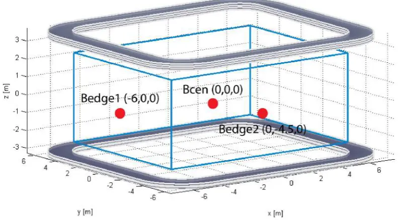
3.1.2 Field Parameters

Figure 3.2 presents the volume of the neutrino detector by the blue box that is located in between the two superconducting magnets, which are depicted in gray. The points that are used to define the size and shape of the magnetic field inside the detector magnet are presented by the red dots. Bcen is located at the center of the detector volume, its position relative to the coordinate system is (0,0,0). Bedge1 and Bedge2 provide the magnetic fields at the center of the short and long edge of the detector volume. Their relative coordinates are (-6,0,0) and (0,-4.5,0).

3.2 Current Density Calculation Method

(19)

[image:19.595.60.545.65.319.2]

(a) Sideview (b) Topview

Figure 3.1: Explanation of the geometry and the parameters used in the optimization study of the detector magnet. Note that the parameter ’hsplit’ is not relevant for the solenoid system (chapter 5) since it exists of only one coil. For the double racetrack system (chapter 4) it is possible to split the coils horizontally and separate them by a vertical distance ’hdeck’.

The operating temperature is mainly determined by the type of cryogent that is used to cool the magnet below the critical temperature. For Niobium Titanium the best way to cool the magnet is to use liquid Helium at its boiling point of 4.2 K. Because the system will be cooled by a pressurized Helium loop, this boiling point is elevated sligthly to 4.5 K, determining the operating temperature of the magnet. The advantage of Magnesium di-boride however is that the cooling costs of the system can be kept low by operating at a higher temperature of approximately 20 K. Such a system would be cooled by Helium gas.

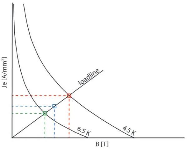
[image:19.595.94.499.532.751.2]

(20)

[image:20.595.146.453.321.564.2]

To calculate the current density at a certain operating temperature a so called loadline fit is performed on the corresponding critical surface slice. First the magnetic peak field is calculated for an arbitrary current density. By making use of the linear relation between the magnetic peak field and the current density, following from Biot-Savart (equation 2.5), a loadline can be drawn by extrapolation of the calculated point through the origin. The intersection of the loadline with the critical surface provides the upper limit for the current density. Superconductivity can only be maintained when the operating current is equal or lower to this upper limit. Beyond this point it is certain the magnet will quench (see section 2.3.3). For safety reasons it is common to include a margin while determining the operating current density. There are two ways to implement a safety margin to the current density calculation (see figure 3.3). The first option is to set a temperature margin. This temperature margin is added to the set operating temperature and therefore changes the critical surface slice that is used for the calculation of the intersection point with the loadline. By adding the temperature margin, the upper limit for the current density is lowered. The second option is to set a loadline margin. This margin is represented by a percentage that is taken on the loadline in order to determine the operating current density. By applying this percentage, the operating point on the loadline will be chosen at a sufficient distance from the critical surface. Commonly only a percentage on the loadline to determine a safe operating current density is applied.

Figure 3.3: Loadline ﬁt performed on a critical surface slice for an operating temperature of 4.5 K. The red square represents the upper limit for the operating point, the blue square represents the operating point after application of a loadline margin and the green square represents the operating point after addition of a 2 K temperature margin to the operating temperature of 4.5 K.

3.3 Optimization Algorithm

As introduced in section 2.4, Field provides the basis for the magnetic ﬁeld calculations. By making use of the text based interface, optimization studies can be performed. This section introduces the numerical method used for the optimization study executed in this report.

3.3.1 Targets and Variables

(21)

The requirements can then be seen as the targets that have to be achieved. The optimization of such a system can be compared to solving a system of non-linear equations. To ensure that there exists only one solution, the number of variables has to be equal to the number of equations. This also applies to the optimization problem. In order to optimize a system with N variables, N so called targets are required. During the optimization, the solver linearises the system of equations at a pre-set start point, after which the solution of the linear system becomes the new start point. After multiple iterations, the system converges to a ﬁnal solution. The optimization study described in this report was implemented in MATLAB and the function fsolve was chosen to perform the optimization. Fsolve solves a system of non-linear equations in the form of f(x) = 0. The Levenberg-Marquadt algorithm[21][22] was selected to perform the calculations. When performing an optimization study, it is important to keep in mind that the optimal set of variables does not always exist within the given bounds. For instance, this could happen when diﬀerent targets are competing. Therefore it is very important to think through the choices of targets and variables before running an optimization.

3.3.2 Parameter Sweep

Next to the parameters that are used as a variable for the achievement of a target, a system usually contains other parameters. These remaining parameters can be included in the optimization study in two ways. The first option is to link them to new targets and to run a second optimization around the first one. During this double optimization, the variables in the inner (first) optimization are used to meet specific magnetic field requirements and the variables in the outer (second) optimization are used to obtain a global objective such as the minimization of the conductor volume. This however, is a time consuming process. The variables that are altered in the outer optimization affect the values of the targets of the inner optimization and the other way around. Therefore a lot of optimization cycles have to be run before both the inner and the outer optimization reach the optimal configuration of variables for the system. The second option is to perform a parametric sweep on the remaining parameters. The value of each parameter is varied over a certain range and for every combination a single optimization is performed. The result is an optimal configuration for each combination of remaining parameters. Based on experience, the second option proves to be much more valuable because it provides insight on the influence of the remaining parameters on the system properties, whereas the first option only gives a single optimal configuration for the system. Therefore the optimization towards the magnetic field requirements accompanied by a parameter sweep is chosen as method for this design study.

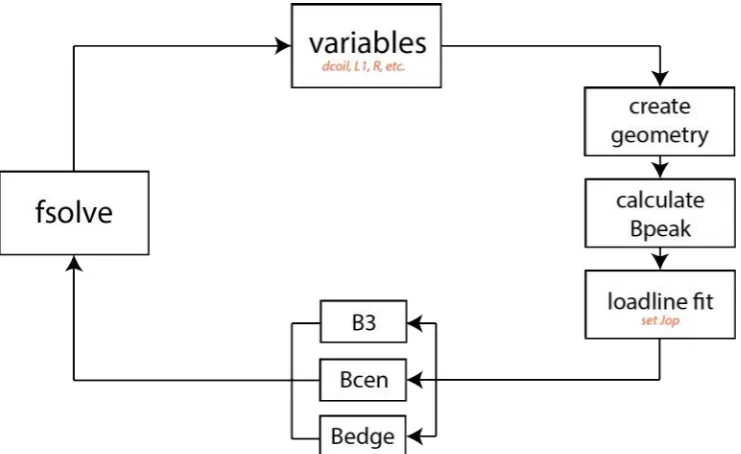
3.3.3 Optimization Cycle

(22)

[image:22.595.114.485.44.271.2]

Figure 3.4: Schematic representation of the optimization process used to meet the ﬁeld requirements.

3.4 Conclusion

(23)

4 Double Racetrack Layout Optimization

This chapter presents the layout optimization performed for the double racetrack configuration. First, the conductor settings are described followed by an overview of the design choices made concerning the geometrical design of the double racetrack system. For the optimization of the double racetrack system two different parametric studies are performed. The aim of both sweeps is to obtain insight in the relation between the geometrical parameters and the properties of the magnetic field. The result of the layout study is a set of optimized models for the double racetrack system. To be able to continue the preliminary design study, a so-called working model is selected. Further analysis is performed with respect to this model.

4.1 Conductor Settings

Since the optimization performed in this report is part of a preliminary design study, the geometrical and electrical properties of the conductor are not well defined. The conductor used for the ATLAS barrel toroid [15] has been successfully implemented and adheres similar requirements for the magnetic field as the neutrino detector. Therefore its properties are used as a first approximation for the optimization study of the racetrack magnet system. The conductor settings used for the layout optimization of the racetrack are listed in table 4.1, 4.2 and 4.3.

Table 4.1: Type and operating parameters of the conductor used for the layout optimization of the double racetrack conﬁguration.

Type Nb-Ti

Operating Temperature 4.5 K

Temperature margin 0 K

I/Ic along the loadline 65 %

Table 4.2: Geometric parameters of the ATLAS barrel toroid conductor which are assumed as a ﬁrst approximation for the superconducting magnet system of the LAr neutrino detector.

Dimensions bare 57.0 * 12.0 mm

insulated 57.8 * 12.8 mm corner radius 57.0 * 12.0 mm

Total cross-section bare 684 mm2

insulated 737 mm2

Aluminium area 632 mm2

(24)

Table 4.3: Cable parameters of the ATLAS barrel toroid conductor which is assumed as a ﬁrst approxi-mation for the superconducting magnet system of the LAr neutrino detector.

Dimensions 22.0 * 2.3 mm

Number of strands 32

Strand diameter 1.30 mm

Filament diameter 0.050 mm

Twist pitch 50 mm

Transposition pitch 140 mm

Cu/Sc ratio 1.30

Section of Nb-Ti 18.5 mm2

Section of Cu 24.0 mm2

4.2 Design Choices

Before performing the optimization a few choices are made concerning the geometrical design of the double racetrack system. These design choices are based on experiences acquired in an earlier stage of the design study and are applied by setting the corresponding parameters to a ﬁxed value. This section explains the reasoning behind these choices. The ﬁxed values for the corresponding parameters are summarized in table 4.4.

Vertical coil height - hcoilPrevious optimization steps revealed that there exists no optimal value for the vertical height of the coils. To reach an optimized system with respect to the ﬁeld requirements, the coil height tends to converge to zero in order to minimize the applied volume of conductor material. Since the size and shape of the conductor put a lower limit on the height of the coils, the value of hcoil is set at the height of a single double pancake coil. This means that the value of hcoil is determined by the combination of the height of two pancakes of the chosen conductor with an insulation layer in between. The short side of the windings is placed along the vertical z-axis.

Two double pancake decks - hdeckPreceding optimization steps showed that to reach the required magnetic field of 1 T in the center of the detector volume, the horizontal coil width (dcoil) had to take up values in the range of 1.00 m to 2.00 m, which is relatively large. Although manufacturing coils of large width is not impossible, it is more favourable to avoid them in order to reduce the total size of the system and to simplify coil production. Additionally the accumulation of forces over the width of the coil reduces, resulting in lower peak pressures. To be able to reduce the horizontal coil width and still meet the magnetic field requirements, the single double pancake coil is replaced by two double pancake coils separated by a fixed distance, hdeck. This ’double double pancake’ coil configuration is similar to the coil construction of the ATLAS barrel toroid system [15]. The vertical distance between the two double pancake decks of the ATLAS barrel toroid is used for the optimization study performed in this section.

Coil corner radius - R The coil corner radius determines the value of the magnetic peak field (at the surface of the racetrack coils) and therefore influences the total required volume of conductor material. Previous optimization steps indicated that to reduce the conductor volume, the coil corner radius had to become very large1_{. Because a large radius increases the size of the total magnet system a suitable value} has to be chosen. For the parametric study of L1 and L2 (section 4.3.1) the radius is set at a fixed value of 1.50 m.

(25)

Coil lengths - L1 and L2 Since placement of the magnet system within the detector volume is not an option, the values for the coil lengths (L1 and L2) can not become smaller than the size of the liquid Argon vessel (see section 1.3).

Table 4.4: Summary of the design choices made for the double racetrack conﬁguration, the corresponding parameters and their values.

Parameter Value Description

hcoil 118.1 mm Vertical coil height

hdeck 50 mm Vertical spacing between two double pancake decks

R∗ _{1.50 m} _{Coil corner radius}

* The value of the coil corner radius is only set to a ﬁxed value for the parametric sweep over L1 and L2 (section 4.3.1).

4.3 Parametric Study

As described in section 3.3.2 the optimization study performed in this report is based on the combination of a single optimization cycle accompanied by a parameter sweep. The parameters are varied over a fixed range of values and for each different combination of parameters the optimizer (section 2.4) attempts to find the optimal design with respect to the set targets. For the double racetrack system two different parametric studies are performed. First, the systems with different values for the inner lengths of the coils (L1 and L2) are optimized. Second, a parametric sweep is performed over the coil radius (R) and the required field at the edge of the detector (Bedgereq). Since both parametric studies have to satisfy the same central field requirement, one could say that the results of both studies are actually the same. This is in fact true, but by looking at the optimization in two ways, different relations between parameters are discovered and different approaches of determining the most suitable model can be applied. If for instance the length of the coils is the limiting factor for the magnet design, the results of the sweep over L1 and L2 should be used to determine an appropriate model. If the field requirement on the edge of the detector is a limiting factor, the results of the sweep over R and Bedgereq should be used to find a suitable model. The results of both parametric studies and an overview of the applied optimization settings are presented in the subsections below.

4.3.1 L1 and L2

For the parametric study of the inner lengths of the coils the values of both L1 and L2 are swept over a speciﬁc range. L1 is varied from 11.00 m to 15.00 m with increments of 1.00 m and L2 is varied from 8.00 m to 13.00 m with increments of 0.50 m. The targets and corresponding variables that are used to perform the optimization for each diﬀerent combination of L1 and L2 are presented in table 4.5.

The aim of this sweep is to obtain knowledge about the relationship between the length of the coil and the magnetic field at the edges of the detector while the value of the magnetic field at the center is kept at a fixed value of 1 T.

(26)

Table 4.5: Explanation of the targets and variables used for the optimization accompanying the parametric study of L1 and L2

Target Variable Description

Bcen = 1 T dcoil By varying the coil width for a fixed coil height the conductor volume will be varied. Since the current density is fixed by the loadline fit, the total current is linearly related to the conductor volume. Therefore variation of the con-ductor volume will influence the magnetic field magnitude at the center of the detector.

B3 = 0 T hsplit Homogeinity of the magnetic field inside the detector can be achieved by forc-ing all the higher harmonics of the magnetic field to be zero (for a detailed explanation of field harmonics see appendix A). The remaining first harmonic, the dipole field, will establish the required uniform field. Since the contribu-tion of higher harmonics reduces exponentially it is sufficient to set the first non-zero harmonic after the dipole to zero. Therefore B3 is set to be zero in order to obtain a homogeneous field. Since the value of B3 is determined by the geometry of the magnet system, the target is coupled to the vertical distance between the two racetrack sets.

detector volume. Therefore, the magnitude of the field at the edge of the detector volume becomes larger. Figure 4.1 shows that the relation between the magnetic field at Bedge1 and L2 changes after L1 becomes larger than 12 m, which is the size of the long side of the detector volume. This change is caused by the fact that for values of L1 smaller than the long side of the detector volume, the magnitude of the magnetic field at Bedge1 is mainly determined by the coil length L2. For values of L1 larger than the long side of the detector volume, the magnitude of the magnetic field at Bedge1 is mainly determined by L1. Large values of L2 lead to an increase of the magnetic peak field and therefore to a decrease of the operating current density (for an explanation see section 4.3.2). Therefore, the magnitude of the magnetic field at Bedge1 is smaller for larger values of L2 (in combination with a value of L1 which is equal or larger than the long side of the detector). This relation can also be recognized in figure 4.2. For small values of L1, an increase in the value of L2 leads to a slightly larger magnetic field at Bedge1. For values of L1 larger than 12 m, an increase in the value of L2 leads to a smaller magnetic field at Bedge1. The figure also illustrates that for very large values of L2, the magnitude of the magnetic field at Bedge1 becomes independent of L2.

(27)

11.0 11.5 12.0 12.5 13.0 13.5 14.0 14.5 15.0 0.3

0.4 0.5 0.6 0.7 0.8 0.9 1.0

L1 [m]

Bedge1

[T]

L2 = 8.0 [m] L2 = 8.5 [m] L2 = 9.0 [m] L2 = 9.5 [m] L2 = 10.0 [m] L2 = 10.5 [m] L2 = 11.0 [m] L2 = 11.5 [m] L2 = 12.0 [m] L2 = 12.5 [m] L2 = 13.0 [m] L2 = 8.0 m

L2 = 13.0 m

Figure 4.1: Magnitude of the magnetic field at Bedge1 as a function of L1 for various values of L2. Note that the way in which L2 influences the magnetic field at Bedge1 changes at the intersection at L1 = 12m.

8.0 8.5 9.0 9.5 10.0 10.5 11.0 11.5 12.0 12.5 13.0 0.3

0.4 0.5 0.6 0.7 0.8 0.9 1.0

L2 [m]

Bedge1

[T]

L1 = 11.0 [m] L1 = 12.0 [m] L1 = 13.0 [m] L1 = 14.0 [m] L1 = 15.0 [m]

L1 = 11.0 m

L1 = 15.0 m

(28)

11.0 11.5 12.0 12.5 13.0 13.5 14.0 14.5 15.0 0.3

0.4 0.5 0.6 0.7 0.8 0.9 1.0

L1 [m]

Bedge2

[T]

L2 = 8.0 [m] L2 = 8.5 [m] L2 = 9.0 [m] L2 = 9.5 [m] L2 = 10.0 [m] L2 = 10.5 [m] L2 = 11.0 [m] L2 = 11.5 [m] L2 = 12.0 [m] L2 = 12.5 [m] L2 = 13.0 [m] L2 = 8.0 m

L2 = 13.0 m

Figure 4.3: Magnitude of the magnetic ﬁeld at Bedge2 as a function of L1 for various values of L2. Note that the magnitude of the magnetic ﬁeld at Bedge2 is independent of the value of L1.

8.0 8.5 9.0 9.5 10.0 10.5 11.0 11.5 12.0 12.5 13.0 0.3

0.4 0.5 0.6 0.7 0.8 0.9 1.0

L2 [m]

Bedge2

[T]

L1 = 11.0 [m] L1 = 12.0 [m] L1 = 13.0 [m] L1 = 14.0 [m] L1 = 15.0 [m]

(29)

4.3.2 R and Bedgereq

For the parametric study of the coil radius and the required value of the magnetic field at the edges of the detector volume the values of both R and Bedgereq are swept over a specific range. R is varied from 1.00 m to 2.00 m with increments of 0.50 m and Bedgereq is varied from 0.500 T to 0.900 T with increments of 0.025 T. The targets and corresponding variables that are used to perform the optimization for each different combination of R and Bedgereq are presented in table 4.6.

Table 4.6: Explanation of the targets and variables used in/for the parametric study of R and Bedgereq

Target Variable Description

Bcen = 1 T dcoil By varying the coil width for a fixed coil height the conductor volume will be varied. Since the current density is fixed by the loadline fit, the total current is linearly related to the conductor volume. Therefore variation of the con-ductor volume will influence the magnetic field magnitude at the center of the detector.

B3 = 0 T hsplit Homogeinity of the magnetic field inside the detector can be achieved by forc-ing all the higher harmonics of the magnetic field to be zero (for a detailed explanation of field harmonics see appendix A). The remaining first harmonic, the dipole field, will establish the required uniform field. Since the contribu-tion of higher harmonics reduces exponentially it is sufficient to set the first non-zero harmonic after the dipole to zero. Therefore B3 is set to be zero in order to obtain a homogeneous field. Since the value of B3 is determined by the geometry of the magnet system, the target is coupled to the vertical distance between the two racetrack sets.

Bedge1 L1 In between the two racetrack coils there exists a zone where the magnetic fields of both coils cancel each other. The distance between this zone and the edge of the detector volume is related to the magnitude of the magnetic field at the edge of the detector volume. By changing the length of the coil in the x-direction (L1), the distance between the short edge of the detector volume and the cancellation zone is varied. Therefore variation of L1 will influence the magnitude of the magnetic field at Bedge1.

Bedge2 L2 In between the two racetrack coils there exists a zone where the magnetic fields of both coils cancel each other. The distance between this zone and the edge of the detector volume is related to the magnitude of the magnetic field at the edge of the detector volume. By changing the length of the coil in the y-direction (L2), the distance between the long edge of the detector volume and the cancellation zone is varied. Therefore variation of L2 will influence the magnitude of the magnetic field at Bedge2.

The result of the combination of the parametric sweep and optimization is a list of 85 optimized models that all satisfy the imposed magnetic field requirements. The geometric design, field specifications and other important system properties are summarized in appendix B.1.

(30)

seen in figure 4.1 and figure 4.4. Since relatively large coils are needed to produce a large magnetic field at the edge of the detector volume, a larger volume of conductor material is necessary to create these fields.

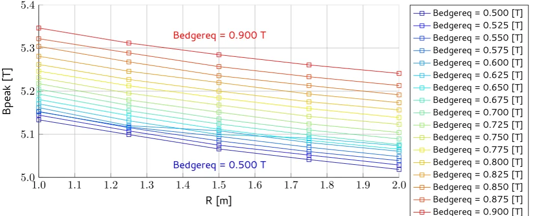
[image:30.595.49.563.537.747.2]

The relation between the magnetic peak field (Bpeak), the coil corner radius (R) and the required magnetic field at the edges of the detector volume (Bedgereq) is illustrated by figure 4.7 and 4.8. Both figures show that for all values of Bedgereq, the magnitude of magnetic peak field becomes smaller for increasing values of the radius. This can be explained by the fact that in the corners where the short and long sides of the racetrack meet, both coils contribute to the overall magnetic field, which therefore becomes higher. By adding a radius between the coils, the distance between the two meeting sides becomes larger, their contributions to the overall magnetic field in the corner drop and therefore the magnetic peak field becomes smaller. Figure 4.7 clearly shows that the effect of the radius increase on the magnitude of the magnetic peak field becomes smaller for larger values of R. Both figures also show that for all values of R, the magnitude of the magnetic peak field becomes larger for increasing values of Bedgereq. In order to produce a larger magnetic field at the edges of the detector, the coils have to be placed at a larger distance from the detector volume (see table 4.6). When L1 and L2 are increased, the operating current density needed to create the required magnetic field of 1 T in the center of the detector goes up. Therefore, the contributions to the magnetic field in the corners of the coils increase and the magnetic peak field becomes larger.

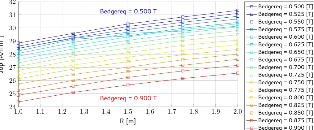
Figure 4.9 and figure 4.10 present the relation between the operating current density (Jop), the coil corner radius (R) and the required magnetic field at the edges of the detector volume (Bedgereq). Both graphs illustrate that the operating current density becomes larger for increasing values of the radius and that it becomes smaller for increasing values of Bedgereq. As explained in section 2.1, the operating current density is fixed by the value of the magnetic peak field. Parameters that influence the magnitude of the magnetic peak field will therefore also affect the value of the operating current density. An increasing corner radius results in a smaller magnetic peak field and therefore a larger operating current density. An increasing required value for the magnetic field at the edge of the detector volume causes the magnetic peak field to become larger and therefore the operating current density decreases.

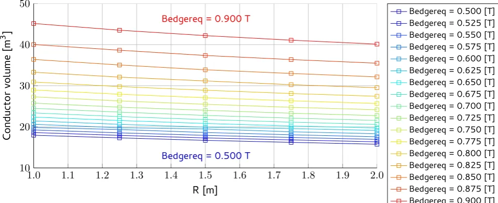
1.0 1.1 1.2 1.3 1.4 1.5 1.6 1.7 1.8 1.9 2.0 10 20 30 40 50 R [m] Conductor volume [m 3 ]

Bedgereq = 0.500 [T] Bedgereq = 0.525 [T] Bedgereq = 0.550 [T] Bedgereq = 0.575 [T] Bedgereq = 0.600 [T] Bedgereq = 0.625 [T] Bedgereq = 0.650 [T] Bedgereq = 0.675 [T] Bedgereq = 0.700 [T] Bedgereq = 0.725 [T] Bedgereq = 0.750 [T] Bedgereq = 0.775 [T] Bedgereq = 0.800 [T] Bedgereq = 0.825 [T] Bedgereq = 0.850 [T] Bedgereq = 0.875 [T] Bedgereq = 0.900 [T]

Bedgereq = 0.500 T

Bedgereq = 0.900 T

(31)

0.50 0.55 0.60 0.65 0.70 0.75 0.80 0.85 0.90 10 20 30 40 50 Bedgereq [T] Conductor volume [m 3 ]

R = 1.00 [m] R = 1.25 [m] R = 1.50 [m] R = 1.75 [m] R = 2.00 [m]

R = 2.00 m

[image:31.595.47.532.47.253.2]

R = 1.00 m

Figure 4.6: Conductor volume (Vc) as a function of the required magnetic ﬁeld at the edges of the detector volume (Bedgereq) for various values of the coil corner radius (R).

1.0 1.1 1.2 1.3 1.4 1.5 1.6 1.7 1.8 1.9 2.0 5.0

5.1 5.2 5.3 5.4

R [m]

Bpeak

[T]

Bedgereq = 0.500 [T] Bedgereq = 0.525 [T] Bedgereq = 0.550 [T] Bedgereq = 0.575 [T] Bedgereq = 0.600 [T] Bedgereq = 0.625 [T] Bedgereq = 0.650 [T] Bedgereq = 0.675 [T] Bedgereq = 0.700 [T] Bedgereq = 0.725 [T] Bedgereq = 0.750 [T] Bedgereq = 0.775 [T] Bedgereq = 0.800 [T] Bedgereq = 0.825 [T] Bedgereq = 0.850 [T] Bedgereq = 0.875 [T] Bedgereq = 0.900 [T]

Bedgereq = 0.500 T

Bedgereq = 0.900 T

Figure 4.7: Magnetic peak ﬁeld (Bpeak) as a function of the coil corner radius (R) for various values of the required magnetic ﬁeld at the edges of the detector volume (Bedgereq).

4.3.3 General results

At the beginning of this section, a remark was made about the fact that the results of both parametric studies are similar. As an addition to the speciﬁc results for each sweep presented in the preceding subsections, this section will give an overview of the general relations observed for the double racetrack system.

[image:31.595.47.573.319.532.2]

(32)

x-0.50 0.55 0.60 0.65 0.70 0.75 0.80 0.85 0.90 5.0

5.1 5.2 5.3 5.4

Bedgereq [T]

Bpeak

[T]

R = 1.00 [m] R = 1.25 [m] R = 1.50 [m] R = 1.75 [m] R = 2.00 [m]

R = 2.00 m

[image:32.595.52.533.103.310.2]

R = 1.00 m

Figure 4.8: Magnetic peak ﬁeld (Bpeak) as a function of the required magnetic ﬁeld at the edges of the detector volume (Bedgereq) for various values of the coil corner radius (R). The curve deviations are artefacts of the MLFMM algorithm used in this optimization study.

1.0 1.1 1.2 1.3 1.4 1.5 1.6 1.7 1.8 1.9 2.0 24 25 26 27 28 29 30 31 32 R [m] Jop [A/mm 2 ]

Bedgereq = 0.500 [T] Bedgereq = 0.525 [T] Bedgereq = 0.550 [T] Bedgereq = 0.575 [T] Bedgereq = 0.600 [T] Bedgereq = 0.625 [T] Bedgereq = 0.650 [T] Bedgereq = 0.675 [T] Bedgereq = 0.700 [T] Bedgereq = 0.725 [T] Bedgereq = 0.750 [T] Bedgereq = 0.775 [T] Bedgereq = 0.800 [T] Bedgereq = 0.825 [T] Bedgereq = 0.850 [T] Bedgereq = 0.875 [T] Bedgereq = 0.900 [T] Bedgereq = 0.900 T

Bedgereq = 0.500 T

[image:32.595.55.562.488.698.2]

(33)

and y-axis. When L1 and L2 become larger, this angle changes and B3 will no longer be zero.2 _{In order} to establish the same optimal angle between the coils and the axes, hsplit should be increased.

Furthermore, the data tables show that the horizontal width of the coils (dcoil) becomes larger for in-creasing coil lengths (L1 and L2). Due to the inin-creasing distance between the coils and the detector a larger current is necessary to meet the magnetic field requirements at the center of the detector vol-ume. Since the current density is limited by the critical surface (section 2.1), the only way to achieve the required magnetic field is to increase the conductor volume. Since the vertical coil height is fixed (section 4.2), the conductor volume can only be increased by increasing the horizontal width of the coils. Therefore, larger coil lengths lead to an increasing coil width and a larger conductor volume.

4.4 Working Model and Analysis

The parametric study presented in section 4.3 resulted in a list of optimized models for the double racetrack system. The choice for an optimal design has to be based on the ﬁnal requirements for the neutrino detector magnet, which are at present not fully deﬁned. Therefore an additional iteration with the people designing the detector itself is necessary. The results presented in this report serve as a basis for such an iteration and form a starting point for future design studies.

To be able to continue the preliminary design study of the double racetrack magnet a so-called working model is selected from the set of optimized systems of the parameter sweep over R and Bedgereq. All further analysis will be performed with respect to this model. The system that is chosen as a working model is the system with id number 43 which is listed in the data tables in appendix B.1. Table 4.7 gives an overview of the properties of the selected working model.

4.4.1 Magnetic Field

Figures 4.11 and 4.12 present a contour plot of the magnetic field magnitude on the cross section of the double racetrack working model for the xz and yz-direction respectively. In both figures, the detector volume is indicated by a black rectangle. It can be seen from both figures that the magnitude of the magnetic field in the detector volume is homogeneous to a large extent, which was one of the field requirements. However it is important to note that the presented cross sectional slices only provide information about the magnetic field magnitude in the center of the detector volume.

4.4.2 Magnetic peak ﬁeld reduction

Since the magnetic peak ﬁeld (Bpeak) determines the operating current density and therefore directly

influences the volume of conductor that is needed to satisfy the magnetic field requirements, it could be beneficial to reduce its magnitude. Next to a cost reduction, a decrease of the volume of conductor also leads to a decrease of the coil widths (dcoil) and therefore reduces the dimensions of the total system. This section presents the influence of three different design adjustments on the magnitude of the magnetic peak field of the double racetrack working model.

Addition of dummyturns

A dummyturn is a spacer that is inserted between the conductor windings at the inner edge of a coil (see ﬁgure 4.14). It is usually designed as a fake coil winding which creates a certain distance between the

(34)

0.50 0.55 0.60 0.65 0.70 0.75 0.80 0.85 0.90 24 25 26 27 28 29 30 31 32 Bedgereq [T] Jop [A/mm 2 ]

R = 1.00 [m] R = 1.25 [m] R = 1.50 [m] R = 1.75 [m] R = 2.00 [m]

R = 1.00 m

[image:34.595.50.533.66.273.2]

R = 2.00 m

Figure 4.10: Operating current (Jop) as a function of the required magnetic ﬁeld at the edges of the detector volume (Bedgereq) for various values of the coil corner radius (R). The curve deviations are artefacts of the MLFMM algorithm used in this optimization study.

Table 4.7: Summary of the properties of the selected working model for the double racetrack system.

Symbol Value Description

L1 12.68 m Coil length in the x-direction

L2 9.84 m Coil length in the y-direction

hsplit 6.01 m Distance between the two racetrack coils in the z-direction

R 1.50 m Coil corner radius

dcoil 1.05 m Horizontal coil width

hcoil 0.1181 m Vertical coil height

hdeck 0.05 m Vertical spacing between two double pancake

decks

Bcen 1.0 T Magnitude of the magnetic ﬁeld at the center of the detector volume

Bedge1 0.7 T Magnitude of the magnetic ﬁeld at the center of the short edge of the detector volume

Bedge2 0.7 T Magnitude of the magnetic ﬁeld at the center of the long edge of the detector volume

B3 -4.18e-06 T Magnitude of the third harmonic ﬁeld inside the detector volume

Vc 22.78 m3 _{Total conductor volume}

Bpeak 5.14 T Magnitude of the magnetic peak ﬁeld at the sur-face of the racetrack coils

Jop 28.81 A/mm2 _{Operating current}

I/Ic 65 % Percentage along the loadline

Estored 1647.78 MJ Stored Energy

L 6.907 H Total Inductance

R

Bz dV 548.32 Tm3 Volume integral over the detector volume for the

[image:34.595.89.507.393.777.2]

(35)

[image:35.595.101.492.72.331.2]

Figure 4.11: Contour plot of the magnetic ﬁeld magnitude [T] in the xz-plane of the racetrack working model evaluated at y = 0. The detector volume is indicated by the black rectangle.

[image:35.595.100.492.433.728.2]

(36)

individual conductor windings of a superconducting coil. The concept of dummyturns has been success-fully implemented in the ATLAS End Cap Toroids [23]. To obtain insight in the influence of dummyturns on the magnitude of the magnetic peak field of the double racetrack working model, a parametric sweep is performed. The amount of dummyturns is varied from 0 to 10 and similar to section 4.3.2 the de-sign is optimized with respect to the set targets, which are (for comparison) equal to the magnetic field properties of the working model (see table 4.7). During the optimization, all other parameters are kept constant.

The relation between the number of dummyturns and the magnitude of Bpeakis presented by ﬁgure 4.13.

It can be seen that the addition of dummyturns decreases the magnitude of the peak field, which is also illustrated by figure 4.14. This decrease is caused by a decrease of the local effective current density, which is the result of the addition of dummyturns to the coil. Although the decrease of Bpeak

is only significant for a large number of dummyturns, figure 4.15 illustrates that the gain in operating current density and the accompanying decrease of the conductor volume are appreciable, even for a small number of dummyturns. Unfortunately, the addition of dummyturns makes coil production more difficult. However, the addition of dummyturns also has a lot of benefits and it could therefore be worthwhile to incorporate them into the double racetrack system.

0 1 2 3 4 5 6 7 8 9 10

4.80 4.85 4.90 4.95 5.00 5.05 5.10 5.15

Number of dummyturns

Bpeak

[image:36.595.76.518.331.532.2]

[T]

Figure 4.13: Magnitude of the magnetic peak ﬁeld of the double racetrack working model as a function of the number of dummyturns.

Variation of hdeck and dshift

For the parametric study performed in section 4.3 the vertical distance between two double pancake decks (hdeck) was fixed at 50 mm, which is similar to the ATLAS Barrel Toroid [15]. The horizontal shift/displacement between two double pancake decks (dshift) was set at 0. To obtain insight in the relation between both distances and the magnitude of the magnetic peak field, two parametric sweeps are performed. Hdeck is varied from 0 mm to 2000 mm with increments of 50 mm and dshift is varied from 0 mm to 1500 mm with increments of 50 mm. Similar to section 4.3.2 the design is optimized with respect to the set targets, which are (for comparison) equal to the magnetic field properties of the working model (see table 4.7). During the optimization, all other parameters are kept constant.

Figure 4.16 illustrates the relation between the magnitude of Bpeak and the vertical and horizontal

(37)

Figure 4.14: Effect of the addition of dummyturns on the magnitude of the magnetic peak field of the double racetrack working model. For each combination of two decks, the values on the left deck (indi-cated in red) refer to the peak field at the inner deck (which is closest to the origin) of a double racetrack configuration.

0 1 2 3 4 5 6 7 8 9 10

18 19 20 21 22 23

Conductor

volume

[m

3 ]

0 1 2 3 4 5 6 7 8 9 10

28 29 30 31 32 33 34 35 36

Jop

[A/mm

[image:37.595.75.528.120.335.2]

2 ]

(38)

decreases when the decks are separated by a larger distance, Bpeakreduces for increasing values of both

hdeck and dshift. However, reduction due to increase of hdeck saturates around a distance of 2000 m since from this distance on, the outer decks of both racetracks are sufficiently near by to influence each other. Since variation of both distances leads to a significant reduction of Bpeak it could be useful to

perform a more detailed study concerning their behaviour.

0 500 1,000 1,500 2,000 4.4

4.6 4.8 5.0 5.2 5.4

hdeck [mm]

Bpeak

[T]

0 250 500 750 1,000 1,250 1,500 4.6

4.7 4.8 4.9 5.0 5.1 5.2

dshift [mm]

Bpeak

[T]

Figure 4.16: Magnitude of the magnetic peak ﬁeld as a function of hdeck and dshift for the double racetrack working model

4.5 Conclusion

(39)

5 Solenoid Layout Optimization

This chapter presents the layout optimization performed for the solenoid conﬁguration. First, the conduc-tor settings are described followed by an overview of the design choices made concerning the geometrical design of the solenoid system. The optimization study of the solenoid system is a combination of a single optimization cycle accompanied by a parameter sweep. The aim of this sweep is to obtain insight in the relation between the geometrical parameters of the system and the properties of the magnetic ﬁeld. The result of the layout study is a set of optimized models for the solenoid system. To be able to continue the preliminary design study, a so-called working model is selected. Further analysis is performed with respect to this model.

5.1 Conductor Settings

Similar to the double racetrack configuration, part of the properties of the conductor of the ATLAS barrel toroid are used as a basis for the optimization study of the solenoid magnet system. The only difference with respect to the ATLAS barrel toroid is that Magnesium di-Boride will be used as a conductor instead of Niobium Titanium. Since Magnesium di-Boride can be operated at a larger temperature range than Niobium Titanium, the operating temperature for the solenoid system will be set at 20 K instead of 4.5 K. This higher operating temperature lowers the cooling costs significantly as explained in section 3.2. The conductor settings used for the layout optimization of the solenoid are listed in table 5.1. All other parameters are equal to the racetrack system (see table 4.2 and table 4.3).

Table 5.1: Type and operating parameters of the conductor used for the layout optimization of the solenoid conﬁguration.

Type MgB2

Temperature of bath 20 K

Temperature margin 0 K

I/Ic along the loadline 65 %

5.2 Design Choices

Before performing the optimization study a few choices are made concerning the geometrical design of the solenoid system. These choices are based on experiences acquired in an earlier stage of the design study and are applied by setting the corresponding parameters to a ﬁxed value. This section explains the reasoning behind all design choices. The ﬁxed values for the corresponding parameters are summarized in table 5.2.