Shadow Detection and Removal based on Automatic Threshold and Boundary Analysis

Shadow Detection and Removal based on Automatic

Threshold and Boundary Analysis

Rakesh Kumar Das

Department of ECE, MANIT Bhopal, M.P, India

Madhu Shandilya

Department of ECE, MANIT Bhopal, M.P, India

ABSTRACT

The objects extraction from their background could be a difficult assignment. Since one threshold or structure threshold certainly fails to resolve doubt , in this paper, we have proposed a brand new technique that automatically observe the edge to exactly discriminate pixels as foreground or background using automatic threshold mechanism. By first distinguishing boundary, its associated curvatures, and edge response, used as benchmark to gauge the possible location of the boundary.Results show that the projected technique systematically performs well in various illumination conditions, as well as indoor, outdoor, moderate, sunny, and rainy cases. By an examination with an empirical evidence in every case, the error rate and the shadow detector index indicate a correct detection, that shows substantial improvement as compared with alternative existing ways.

Keywords

Boundary evaluation, curvature, edge, error rate, foreground extraction, gradient map, shadow detector index, threshold.

1.

INTRODUCTION

Shadow removal is fascinating in several things. Shadows square measure common in natural scenes, and that they square measure renowned to complicate several PC vision tasks like image segmentation and object detection. Thus the flexibility to get shadow-free pictures would benefit several PC vision algorithms. Moreover, for aesthetic reasons, shadow removal can benefit image editing and computational photography algorithms. Automatic shadow detection and removal from single pictures, however, very difficult. A shadow is cast whenever an object occludes an illuminant of the scene; it is the outcome of involute interactions between the geometry, illumination, and reflectance present in the scene. Identifying shadows are consequently arduous because of the constrained information about the scene’s properties.

The foreground extraction quandary can be pixel predicated or region predicated. Simple differencing is the most intuitive by arguing that a transmutation at a pixel location occurs when the intensity difference of the corresponding pixels in two images exceeds a certain threshold. However, it is sensitive to pixel variation resulting from noise and illumination changes, which frequently occur in intricate natural environments. A lot of strong strategies [1] –[3] handle noise associate degrees lighting amendment problems with maintaining an accommodative applied mathematics background model.Recently, Tsai and Lai [4] have projected mistreatment freelance part analysis to wear down illumination changes while not background model change.

On the opposite hand, region-based modification detection strategies benefit of interpixel relations, measurement the region characteristics of a picture try at an equivalent element location. For instance, the likelihood ratio test [5] uses a

hypothesis test to decide whether statistics of two corresponding regions come from the same intensity distribution. Although this technique is a lot of proof against noise, it's still fairly sensitive to illumination changes. The shading model (SM) [6] exploits the quantitative relation of intensities within the corresponding regions of two pictures to deal with illumination changes. Liu et al. [7] instructed a change-detection theme that compares circular shift moments (CSMs), that represent the reflectance element of the image intensity, regardless of illumination. However, each the SM and CSM strategies poorly perform over dark regions

Whether the strategy is pixel based or region based, thresholding of the image is more difficult. In several cases, the threshold is chosen by trial and error or empirically. Obviously, a threshold chosen during this method is ineffective for pictures with significantly completely different distributions. As a result, many adaptive threshold choice strategies are projected. a number of these strategies area unit supported histograms. as an example, Otsu’s technique [8] calculates the simplest threshold by minimizing the quantitative relation of intraclass and interclass variations, the isodata formula [9] searches for the simplest threshold by an reiterative estimation of the mean values of the foreground and background pixels, the triangle algorithm [10] notably deals with unimodal histograms, Kita [11] analyzes the characteristics of the ridges of clusters on the joint bar chart, and Sen and Pal [12] select the threshold by using the fuzzy and rough set theories. Another set of approaches is to assume that the distributions of the changes and also the noise of the distinction image area gaussian or Laplacian. as an example, Bruzzone and Prieto [13] shapely the distinction image as a mixture of two gaussian distributions, representing modified and unmodified pixels. The means and variances of the class-conditional distributions are then calculated using expectation–maximization formula. Rosin and Ellis [14] exploited the easy statistics of the median and also the median absolute deviation by presumptuous that less than half the image is in motion. Kapur et al. [15] elite thresholds by virtue of the entropy of the image. grey [16] thought-about the mathematician range, and O’Gorman [17] used image property.

18

2.

PROPOSED METHOD

2.1.Outline

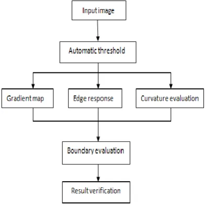
The proposed method consists of three steps as shown in figure 1.1) thresholds selection; 2) boundary evaluation 3) result verification .All these steps are specify in the following sections.

Figure 1.Overview of proposed method

2.2.Thresholds Selection

The neighbourhood valley-emphasis methodology is employed that is planed by Fan and Lei [18]. They were found through experiment that choosing the digital number (T) with the bottom frequency within the valley between the last two peaks gave systematically correct threshold levels for separating the shadow from non shadow region that is shown in Figure.2. a lot of accuracy was obtained from the method by choosing the threshold value that has tiny chance in its neighbourhood space. The method additionally maximizes the

Figure2.(a)Input image.(b) Associated histogram.

between-classes variance in the histogram between the last two peaks (Pe and Pe−1).the following formula is used to find out the threshold:

(1)

Where the probability of the occurrence (i) in an image with (n) as the total number of pixels is defined as

(2)

The entire image represented by a number of distinct levels (L) which is computed as

(3)

The threshold value (T) divides the image pixels into two classes. The probabilities of the two classes are

, (4)

The mean values of the two classes can be computed as

(5)

pt which is the sum of the neighbourhood probability in

interval n =2m+1 for image ( i) is computed as

pt=[p(t−m)+····+p(t−1)+p(t)+p(t+1)+··.+p(t+m)] (6)

Where n is the neighbourhood length, normally is an odd number. The shadow region is accordingly determined from the point (T) to the right end of the histogram. The shadow image is then constructed by giving the value (0) to all shadow pixels and the value (1) to all non-shadow pixels.

2.3.Boundary Evaluation

With refrence to the edge response and curvature to identify

which one is a lot of seemingly to represent true boundary.This is based on three assumptions: 1) The true boundary phase is related to an oversized edge response; 2) the objects’ shapes are usually smooth; and 3) long and convoluted segments are unlikely to be a true boundary. The subsequent sections describe how boundary is evaluated per these assumptions.

a) Finding edge: To evaluate the edge , the method for extracting the edge map EM of the input image I is obtained by the Canny edge detector, and the gradient maps ∇I =(∇xI,∇yI) of I is calculated. Then, the normalized gradient map GM of I is computed as

GM(x,y)

∇

(7)

Where

(8)

The Edge map of the input images is shown in Fig. 3

b) Curvature evaluation: The curvature of point C(n)=(x(n),y(n)) is calculated by

K(n)= (9)

Where C denotes the edge response of a boundary segment C, C(n) denotes the nth point of C, and each dot denotes a differentiation with respect to n. The total curvature of C is calculated as the sum of curvature at each point

(10)

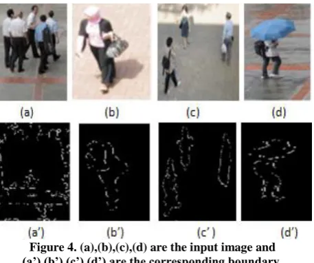
Where Nc is the number of points on C,We consider the total curvature instead of the mean curvature as it is more representative in that a small Kc indicates a concise length and

a smooth C, which are the characteristics of a true boundary which is shown in Fig.4.

Figure 4. (a),(b),(c),(d) are the input image and (a’),(b’),(c’),(d’) are the corresponding boundary.

2.4.Result verification

The resulting boundary is usually a reasonable estimation of the ground truth. However, false-positive regions may still be present in the result. We use edge map as a measure to remove these regions and a median filter of size 3×3 is applied to remove the noise. The result of median filter of the example image is shown in Fig. 5.

Figure 5. (a),(b),(c),(d) are the input image and (a’),(b’),(c’),(d’) are the results of median filter.

3.

RESULTS AND ANALYSIS

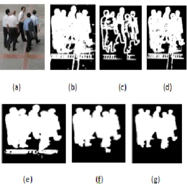
The projected technique has been evaluated on images of various illumination conditions, as well as indoor, outdoor, moderate and rainy cases. Some other change detection methods, including the minimum description length(MDL),the SM [6], the derivative model (DM) [6], Li’s texture-based approach [19], and Lu’s[20 ]are chosen for comparison. We tend to selected the one that made all-time low error rate when compared with the ground truth. The segmentation results are displayed in Figure s. 6–9 with the subserquent layout: (a) input image I (b) the result of MDL, (c) the result of SM, (d) the result of DM, (e) the result of Li’s method, (f) the result of Lu’s method, (g) the result of the proposed method.

The results are also quantitatively computed in terms of the error rate and shadow detector index,the error rate is is defined by the following formula:

Error Rate =(FP+ FN)/(TP +FP+ FN)×100% (11)

where FP stands for the number of no-change pixels incorrectly detected as change, FN stands for the number of change pixels incorrectly detected as no-change,and TP represents the number of change pixels correctly detected. .The error rates for the proposed method and other existing methods are summarized in Table I.

The shadow detector index(SDI) is calculated as[21]:

(12)

Where R, G, and B are normalized components of red, green, and blue bands, respectively. PC1 is a normalized component of the first principal component. The SDI index for the proposed method and other existing methods are shown in Table II. The overall accuracy is calculated by the following formula

20 Figure 6.case-1 group of people with moderate

illumination

In case 2 (see Figure . 7), the shadow is strong. The MDL result is noisy and heavily full of the shadow. The results of all the strategies, except those of the planned methodology, are affected by shadow boundaries, and only Li’s method can potentially delete the shadow edges by acting a morphological opening operation, where as SM and DM cannot because the other foreground pixels will be removed at the equivalent time. The prevalance of the planned methodology over alternative strategies is that it removes additional shadow pixels.

Figure 7.case-2 single person with strong illumination

n Case 3 (see Figure. 8) contains a scene whereever the higher half below the sun and also the lower half is within the shadow of a flyover, forming a high-contrast scenario. Li’s method performs quite well, The proposed method successfully extracts the contour, removes the shadow.

Figure 8.case-3 strong illumination with more contrast

In Case 4 (see Figure. 9) is taken in the rain.Due to the use of a automatic- threshold, that is insensitive to the raindrop reflections. All the other methods are severely affected by the raindrops. MDL, SM, DM and Lu,s are also affected by the shadow.

Figure 9.case-4 reflection in rain

Table 1Error rate of the proposed method compared with existing methods

Error

Rate(%) MDL SM DM LI

LU Proposed

Case 1 36.8 47.0 31.0 22.0 5.0 4.2

Case 2 44.4 32.9 32.0 22.0 7.3 6.5

Case 3 28.8 27.2 24.1 14.7 5.2 4.7

Case 4 63.9 49.3 40.9 30.0 6.8 5.9

Table 2sdi Of The Proposed Method Copmpared With Existing Methods

Input Image of Fig.5.

Overall Accuracy[21]

Overall Accuracy proposed

(a) 97.96 98.01

(b) 96.73 97.21

(c) 96.76 97.09

4.

CONCLUSION

A novel extraction technique supported automatic thresholding and boundary evaluation has been proposed . By using automatic threshold, the problem is reduced,although thresholding is globally performed, the utilization of edge response and curvature helps to boost boundary accuracy throughout the analysis stage. By applying automatic threshold strategy which automatic detect the edge, the regions along the boundary are effectively removed. The classification error rate and shadow detector index compares well with other existing methods.

5.

Acknowledgments

The authors would like to acknowledge Manjula Devi for their exemplary guidance, monitoring and constant encouragement throughout the making of this paper. The authors would also like to acknowledge Santosh Mishra for his help and advice on paper writing.

6.

REFERENCES

[1] C. R. Wren, A. Azarbayejani, T. Darrell, and A Pentland, “Pfinder: Realtime tracking of the human body,” EE Trans. Pattern Anal. Mach. Intell., vol. 19, no. 7, pp. 780–785, Jul. 1997.

[2] C.Stauffer and W. E. L. Grimson, “Learning patterns of activity using real- timetracking, ”IEEETrans. Pattern Anal. Mach.Intell.,vol.22,no.8, pp. 246–252, Aug. 2000.

[3] A.Elgammal,R.Duraiswami,D.Harwood,andL.S.Davis, “Background and foreground modeling using non parametric kernel density estimation for visual surveillance,” Proc. IEEE, vol. 90, no. 7, pp. 1151– 1163, Jul. 2002.

[4] D. M. Tsai and S. C. Lai, “Independent component analysis-based background subtraction for indoor surveillance,” IEEE Trans. Image Process., vol. 18, no. 1, pp. 158–167, Jan. 2009.

[5] Y. Z. Hsu, H. Nagel, and G. Reckers, “New likelihood methods for change detection in image sequences,” Comput. Vis. Graph. Image Process., vol. 26, no. 1, pp. 73–106, Apr. 1984.

[6] K. Skifstad and R. Jain, “Illumination independent change detection for real world image sequences,”. Vis., Graph. Image Process., vol. 46, no. 3, pp. 387–399, Jun. 1989.

[7] S. Liu, C. Fu, and S. Chang, “Statistical change detection with moments under time-varying illumination,”IEEE Trans. Image Process., vol. 7, no. 9, pp. 1258–1268, Sep. 1998.

[8] Otsu,“A threshold selection method from gray-level histograms,” IEEETrans.Syst.,Man,Cybern.,vol.SMC-,no.1,pp.62–66,Jan.1979.

[9] T. W. Ridler and S. Calvard, “Picture thresholding using an iterative selection method,” IEEE Trans. Syst.,Man, Cybern., vol. SMC-8, no. 8, pp. 630–632, Aug. 1978.

[10]G. W. Zack, “Automatic measurement of sister chromatid exchange frequency,” J. Histochem. Cytochem. vol. 25, no. 7, pp. 741–753, 1977.

[11]Y. Kita, “Change detection using joint intensity histogram,” in Proc. Int. Conf. Pattern Recog., Hong Kong, 2006, pp. 351–356.

[12]D. Sen and S. K. Pal, “Histogram thresholding using fuzzing and rough measures of associated error,” IEEE Trans. Image Process., vol. 18, no. 4, pp. 879–888, Apr. 2009.

[13]L. Bruzzone and D. F. Prieto, “Automatic analysis of the difference image for unsupervised change detection,” IEEE Trans. Geosci. Remote Sens., vol. 38, no. 3, pp. 1171–1182, May 2000.

[14]P.L.RosinandT.Ellis,“Imagedifferencethresholdstrategies andshadow detection,” in Proc. Brit. Mach. Vis. Conf., Birmingham, U.K., 1995, pp. 347–356.

[15]J. N. Kapur, P. K. Sahoo, and A. K. C. Wong, “A new method for graylevel picture thresholding using the entropy of the histogram,” Comput. Vis. Graph. Image Process., vol. 29, no. 3, pp. 273–285, 1985.

[16]S. B. Gray, “Local properties of binary images in two dimensions,” IEEE Trans. Comput., vol. C-20, no. 5, pp. 551–561, May 1971.

[17]L. O’Gorman, “Binarization and multi-thresholding of document images using connectivity,” in Proc. Symp. Document Anal. Inf. Retrieval, Las Vegas, NV, 1994, pp. 237–252.

[18]J.-L. Fan and B. Lei, “A modified valley-emphasis method for automatic thresholding,” Pattern Recognit. Lett., vol. 33, no. 6, pp. 703–708, 2012.

[19]L. Li and M. K. H. Leung, “Integrating intensity and texture differences for robust change detection,” IEEE Trans. Image Process., vol. 11, no. 2, pp. 105–112, Feb. 2002.

[20]Lu Wang and Nelson H. C. Yung,’’Extraction of moving objects from their background based on multiple adaptive thresholds and boundary evaluation,’’ IEEE Trans. Intelligent transportation systems., vol. 11, no. 1,pp.40-51, march 2010.