Efficiency of Multilayer Perceptron Neural Networks Powered by Multi Verse Optimizer

(1)

Efficiency of Multilayer Perceptron Neural Networks

Powered by Multi-Verse Optimizer

Abdullah M. Shoeb

Computer Science Department Faculty of Computers and Information

Fayoum University, Egypt

Mohammad F. Hassanin

Computer Science Department Faculty of Computers and Information

Fayoum University, Egypt

ABSTRACT

The models of artificial neural networks are applied to find solutions to many problems because of their computational power. The paradigm of multi-layer perceptron (MLP) is widely used. MLP must be trained before using. The training phase represents an obstacle in the formation of the solution model. Back-propagation algorithm, among of other approaches, has been used for training. The disadvantage of Back-propagation is the possibility of falling in local minimum of the training error instead of reaching the global minimum. Recently, many metaheuristic methods were developed to overcome this problem. In this work, an approach to train MLP by Multi-Verse Optimizer (MVO) was proposed. Implementing this approach on seven datasets and comparing the obtained results with six other metaheuristic techniques shows that MVO exceeds the other competitors to train MLP.

General Terms

Metaheuristic techniques to train multi-layer perceptron.

Keywords

Training neural network, back propagation, multi-verse optimizer, classification.

1. INTRODUCTION

The models of artificial neural networks (ANNs) have considerable power to solve problems in wide range of domains. ANN is composed of interconnected simple processing elements (perceptrons) that forming a parallel processing model. From the perceptron, as a building block, sophisticated structures of ANNs can be developed. The technique of connection and arrangement of perceptrons affects the final structure of the ANN. In most cases, many perceptrons are arranged into layers. If there is a feedback connection, a recurrent ANN is obtained. In most cases, the category of underlying problem determines the type of ANN that to be used to solve it.

To take advantage of an ANN, it must perform two phases. The first phase is dedicated to establishing the ANN. In the establishing process, setting the parameters that define the kind and shape of the ANN is a major step. These parameters include for example how many layers are used and the size of each layer. During the first phase, interconnections' weights must be assigned. Training process is carried out by modifying weights iteratively. The desired goal of ANN learning is computing the best matrix of weights to minimize the performance error. After that phase, the ANN can be operated on the problem to get the results.

The training can be carried in either supervised, unsupervised, or reinforcement manner. In supervised training, ANN is supplied by input and the desired output. The difference

between the obtained and required outputs guides the process of weights' adjustment. A restricted feedback, evaluation of ANN performance, is allowed in reinforcement training. Unsupervised training deprives the ANN from the feedback completely.

The multilayer feed-forward ANNs accompanied by two more layers can work out with issues of classification and recognition regardless of the intrinsic difficulty [1]. Classically, MLP is trained by back-propagation algorithm (BPA). BPA uses the errors coming from supervised training to iteratively improve weights matrix to decrease the NN gross error continuously.

BPA shows good performance when handling wide range of questions, but it suffers an important weakness. The algorithm is based on gradient descent concept. So, if the initial weights, or even any coming weights, lead to the error valley that differs from the global one, the training process will be prematurely stop at this local minimum. To avoid that, usually initial solution was randomized and also different groups of initial weights were used. This work is devoted to use multi-verse optimizer to keep away from BPA local minimum. Many nature-inspired heuristics algorithms have been discovered recently to train ANN. Among of others metaheuristic methods are Grey Wolf Optimization (GWO) [2, 3], Particle Swarm Optimization (PSO) [4, 5], Genetic Algorithm (GA) [6], Ant Lion Optimizer (ALO) [7], Cuckoo Search (CS) [8, 9], Evolutionary Strategy (ES) [10], and Social Spider Optimization (SSO) [11].

The next sections of the paper are organized as follows. Section 2 is dedicated to cover multi-verse optimizer. The study framework is introduced in section 3. Section 4 discusses the performed simulation and experimental work. Section 5 concludes the study.

2. MLP POWERED BY BPA

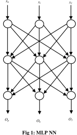
Backpropagation net has the same structure as MLP, see Figure 1, but it is implementing BP learning algorithm. Inputs are provided to the network through, the top, input layer (x1,

xn). Input layer distribute these values to the first hidden layer.

Hidden layer neurons compute weighted sum from the received values. Each neuron passes its own weighted sum to the sigmoid function to calculate its output. These outputs are passes to, the lower, output layer. Output layer uses the same behavior as the hidden layer to compute the outputs, O1, …,

Op.

(2)

[image:2.595.98.233.116.351.2]

from output layer connected neurons. Same argument is applied to the input layer. After ’s calculation, the weights matrix is modified according to some rule.

Fig 1: MLP NN

3. MULTI-VERSE OPTIMIZER

Many theories discuss cosmogony; multi-verse optimizer (MVO) algorithm [12] is inspired from the line of these theories. This algorithm depends on three ideas in that theory. These ideas are white and black holes and wormhole and they are used to continuously enhance a random solution. The first two holes are utilized to inspect the search space. The solution is considered as a universe. As the objects constitute the universe, the variables constitute the solution, so the terms universe and solution will be used interchangeably in this section. MVO founders simulate universe-inflation rate by solution fitness. The algorithm exchanges variables through solutions simply. The variable is switched to a lower fitness solution. To simulate randomness, the algorithm allows variables to be changed between solutions arbitrarily all the time.

successively, MVO improves the achieved solution as follows [12]:

Let n be the number of alternative solutions. Let d be the number of variables in each solution.

Arrange the solutions according to their fitness. Pick one solution randomly to be the one with a white hole.

where is the variable number n of the solution number m, Ui is solution number i, r1  [0,1], and is the variable number j of kth solution selected randomly.

Randomly exchange objects:

WEP can be computed according to the formula:

where min and max are constants, l and L are the current iteration and number of iterations threshold iteratively. TDR is computed according to the equation:

where p is a constant.

MVO algorithm is ending by attaining a prespecified upper iterations’ threshold.

4. MLP POWERED BY MVO

Training of MLP is an essential part of preparing the network for prediction and classification. The target of this process is to set connections weights that able to answer the problem question. The proposed approach exploits MVO algorithm as a trainer to multilayer feedforward neural network. MLP must be trained over a given sample, so MVO function is supplying better weights successively.

The problem must be represented in a format that accepted by the used meta-heuristic technique. MLP usual training procedure and MVO use the same representation. The connections’ weights are initially assigned uniformly. Training sample is preprocessed prior to entering it to the input layer. After that the weights are improved by MVO. Sigmoid was chosen to be the activation function. The mean squared error (MSE) (E) has been chosen as indicator to stability and convergence. Training was stopped after a specified rounds threshold.

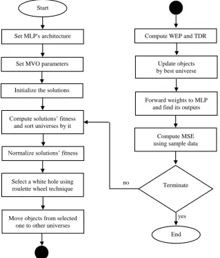
Firstly, the MLP's architecture was specified to solve the study case. Then MVO arguments are adjusted and also initial values of the variables are assigned. Consecutively, solutions are enriched through rounds as follows. Universes inflation rates are computed, arranged, and normalized. A random variable generator selects a supplier universe to move objects out to picker universes utilizing a particular formula. Then, the finest solution updates the other universes. MLP output, of the sample, is found using the evaluated weights. The stability and weights improvements are examined by the mean squared error equation. Figure 2 summarizes the overall steps of the proposed approach.

x1 xi

xn

O1 Ok

(3)

[image:3.595.139.459.73.449.2]

Fig 2: General framework

5. SIMULATION AND EXPERIMENTAL

RESULTS

To explore the strength of the proposed approach, MVO Feedforward Neural Network (MVO-FNN), a set of experiments were performed. The approach was examined for a variety types of problems that require precise classification. The datasets of breast cancer, iris, heart, balloon, and 3-bit XOR was acquired from UCI Machine Learning Repository [13]. Also, two trigonometric function datasets acquired from [14].

MVO was examined against other metaheuristic techniques such as GWO, PSO, SSO, and ACO as swarm techniques, and against ES and GA as evolutionary techniques. The initial parameter values of the studied techniques were assigned according to each algorithm's nature. In all techniques, top number of generations is assigned to be 200. The default initial parameters of MVO and compared algorithms are summarized in Table 1 Finally, the architecture of the MLP is adjusted to obtain the best architecture.

Regarding the classification datasets, the number of attributes is ranged from 3, in the case of 3-bit XOR, up to 22, in the case of heart dataset. The training sample size is ranged from 8 entries, in the case of 3-bit XOR, up to 599 entries, in the case of breast cancer. The number of classes is ranged from 2 – in four datasets – up to 3, in the case of iris.

The architecture of the MLP corresponds to the dataset. The size of input and output layers and the number of dataset attributes are static according to the dataset. While the size of hidden layer is dynamic. The way of determining hidden layer size is unified to be as twice as the number of attributes. Four evaluation metrics have been used to examine the efficiency of the proposed framework. The average (AVE) after 200 iterations was used to measure the capability of local solutions avoidance. Standard deviation was used after the same threshold as indicator for stability. Classification rate was used in the first five datasets to assess the power of the proposed approach relative to other competitors. Finally, test error was used in the function approximation datasets.

5.1 3-Bit XOR Dataset

In this dataset, there are three attributes, the training and testing samples are equally set to 8, and the classes of the problem are two classes. The NN architecture is organized as follows: 3 neurons in the input layer, 6 neurons in the hidden layer, and finally a single neuron in the output layer.

The results of comparison of the proposed approach and the other six techniques for 3-bit XOR dataset are introduced in Table 2 and Figure 3. MVO attains the best average of MSE and SSO comes in the second stage. These results Start

Terminate Set MLP's architecture

yes Set MVO parameters

Initialize the solutions

Compute solutions’ fitness and sort universes by it

Normalize solutions’ fitness

Select a white hole using roulette wheel technique

Move objects from selected one to other universes

Compute WEP and TDR

Update objects by best universe

Forward weights to MLP and find its outputs

Compute MSE using sample data

(4)

Table 1. Parameters’ values of algorithm

Algorithm Parameter Value

MVO

Max. generations 200

Pop. Size XOR and Balloon: 50 and others:150 GWO

Linearly decreased from 2 to 0

Pop. Size XOR and Balloon: 50 and others:150 SSO

PF 0.7

Pop. Size XOR and Balloon: 50 and others:150 PSO

Topology Fully connected

1

w 0.3

Max. rounds 200

Pop. Space XOR and Balloon: 50 and others:150 ACO

τ 1e-06

Q 20

q 1

0.9 0.5

α 1

β 5

Max. iterations 200

Pop. Size XOR and Balloon: 50 and others:150 ES

Λ 10

Σ 1

Pop. Size XOR and Balloon: 50 and others:150 GA

Type Real coded

Selection Roulette wheel

Crossover Single point (probability=1) Mutation Uniform (probability=0.01)

(5)

[image:5.595.316.541.79.393.2]

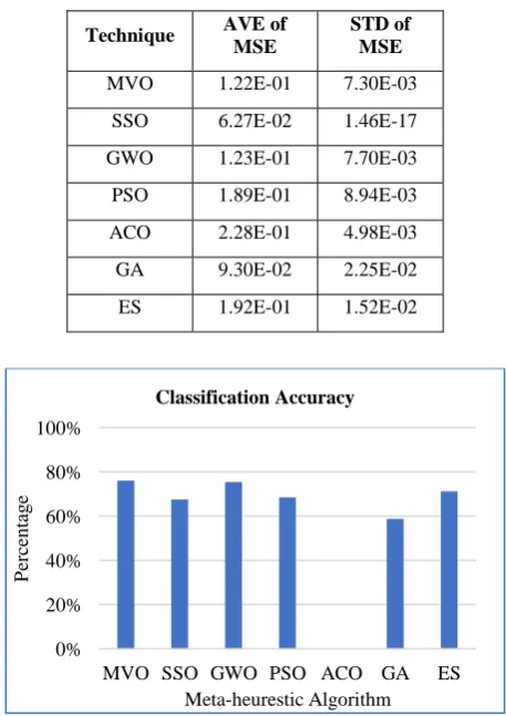
reflect strength of MVO and SSO to keep away from regional valley. Results of GA and GWO are showing them as competitors, with less performance, for MVO and SSO. Regarding stability, SSO and MVO are coming firstly followed by GA. For classification accuracy, MVO, SSO, GWO, and GA are reached 100%, however, ES, ACO, and PSO were unable of do so.

Table 2. 3-Bit XOR outcomes

Technique AVE of

MSE

STD of MSE

MVO 4.50E-10 6.17E-10 SSO 2.81E-05 0.00E+00 GWO 9.41E-03 2.95E-02 PSO 8.41E-02 3.59E-02 ACO 1.80E-01 2.53E-02 GA 1.81E-04 4.13E-04 ES 1.19E-01 1.16E-02

Fig 3: Accuracy of algorithms handling 3-Bit XOR

5.2 Balloon Dataset

In this dataset, there are four attributes, the training and testing samples are equally set to 16, and the classes of the problem are two classes. The NN architecture is organized as follows: 4 neurons in the input layer, 8 neurons in the hidden layer, and finally a single neuron in the output layer.

Figure 4 briefs the outcomes of the various techniques. The classification accuracy reaches its great value at 100% for all techniques which reflects the simplicity of the problem. However, Table 3 shows considerable variation of AVG and STD the error function. As in the previous dataset, GA and MVO attained strong capacity to avoid local optima then SSO and GWO followed them.

Table 3. Balloon outcomes

MSE

STD of MSE

MVO 8.88E-19 1.38E-18 SSO 1.74E-15 0.00E+00 GWO 9.38E-15 2.81E-14 PSO 5.85E-04 7.49E-04 ACO 4.85E-03 7.76E-03 GA 5.08E-24 1.06E-23 ES 1.91E-02 1.70E-01

Fig 4: Accuracy of algorithms handling balloon

5.3 Iris Dataset

In this dataset, there are four attributes, the training and testing samples are equally set to 150, and the classes of the problem are three classes. The NN architecture is organized as follows: 4 neurons in the input layer, 8 neurons in the hidden layer, and finally 3 neurons in the output layer.

[image:5.595.53.279.160.478.2]

This dataset is not simple as the two preceding datasets; hence it can distinguish clearly between the considered techniques. Again, MVO demonstrates its capability to keep away from the regional valley superior to the other techniques with GA as a successor. MVO exceeds the other techniques in the classification rate, as presented in Figure 5. The juxtaposition of error function’s AVGs is carried out in Table 4.

Table 4. Iris outcomes

MSE

STD of MSE

MVO 1.82E-02 4.30E-03 SSO 2.10E-02 3.66E-18 GWO 2.29E-02 3.20E-03 PSO 2.29E-01 5.72E-02 ACO 4.06E-01 5.38E-02 GA 8.99E-02 1.24E-01 ES 3.14E-01 5.21E-02 0%

20% 40% 60% 80% 100%

MVO SSO GWO PSO ACO GA ES

P

erc

en

tag

e

Meta-heurestic Algorithm Classification Rate

0% 20% 40% 60% 80% 100%

P

erc

en

tag

e

[image:5.595.343.515.567.728.2] [image:5.595.344.514.572.727.2]

(6)

[image:6.595.54.282.70.229.2]

Fig 5: Accuracy of algorithms handling iris

5.4 Breast Cancer Dataset

In this dataset, there are nine attributes, the training sample is set to 599, testing sample is set to 100, and the classes of the problem are two classes. The NN architecture is organized as follows: 9 neurons in the input layer, 18 neurons in the hidden layer, and finally a single neuron in the output layer.

[image:6.595.313.542.244.568.2]

The current dataset is fairly difficult; so a lot of techniques failed to categorize the test sample with acceptable rate. Figure 6 shows that MVO, GWO, GA, and SSO techniques attains high classification rate, in the same presented order. GA and SSO obtained the same rate by 98%. MVO was achieved the highest rate by 99.7% superior to GWO. Table 5 introduces the error function AVG, MVO was achieved an advanced position. As a final notice, the results of some techniques declined down, and this is due to the fixed number of iterations.

Table 5. Breast cancer outcomes

MSE

STD of MSE

MVO 1.30E-03 5.55E-05 SSO 1.60E-03 2.28E-19 GWO 1.20E-03 7.45E-05 PSO 3.49E-02 2.47E-03 ACO 1.35E-02 2.14E-03 GA 3.03E-03 1.50E-03 ES 3.20E-02 3.07E-03

Fig 6: Accuracy of algorithms handling breast cancer

5.5 Heart Dataset

In this dataset, there are 22 attributes, so it is the most complicated dataset. The training sample is set to 80, testing sample is set to 187, and the classes of the problem are two classes. The NN architecture is organized as follows: 22 neurons in the input layer, 44 neurons in the hidden layer, and finally 1 neuron in the output layer.

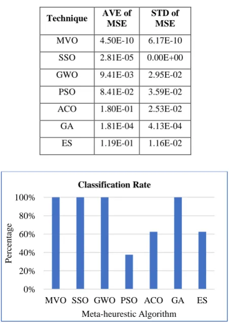
It has more than double the number of attributes in the previous dataset. MVO still has the top classification rate compared to all other techniques as shown in Figure 7. GWO technique comes in the next stage after MVO. The classification accuracy for ACO is equals to zero. Table 6 shows that SSO attain the least value of MSE average then GA and MVO respectively.

Table 6. Heart outcomes

MSE

STD of MSE

Fig 7: Classification accuracy for heart dataset

5.6 Cosine Function Dataset

In this dataset, the training and testing samples are equally set to 30. The NN architecture is organized as follows: 1 neuron in the input layer, 10 neurons in the hidden layer, and finally 1 neuron in the output layer.

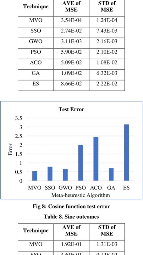
Figure 8 presents the test error of cosine approximation function. In this case, and the following one, the previous categorization accuracy metric will not use as a measure of the power of the technique; a test error evaluation measure is utilized. MVO is very robust as it was achieved least value of both MSE AVG and test error. GWO was coming after MVO in both metrics. Moreover, MVO was attained the highest stability rate, see Table 7.

0% 20% 40% 60% 80% 100%

P

erc

en

ta

g

e

0% 20% 40% 60% 80% 100%

P

erc

en

ta

g

e

0% 20% 40% 60% 80% 100%

P

erc

en

tag

e

[image:6.595.55.282.442.748.2]

(7)

5.7 Sine Function Dataset

In this dataset, the training sample is set to 120, and testing sample is set to 240. The NN architecture is organized as follows: 1 neuron in the input layer, 10 neurons in the hidden layer, and finally 1 neuron in the output layer.

[image:7.595.315.543.72.229.2]

Table 8 shows the obtained results of sine function. MVO was attained least MSE AVG which reflects the capability of MVO to keep away of regional optimum. In the same time MVO was achieved the better STD which proves stability. Also, the proposed approach success to get the minimum test error, see Figure 9. Hence it outperforms the other competitor approaches in this dataset.

Table 7. Cosine outcomes

MSE

STD of MSE

[image:7.595.53.281.229.635.2]

Fig 8: Cosine function test error

Table 8. Sine outcomes

MSE

STD of MSE

Fig 9: Sine function test error

From the obtained experiments outcomes, some observations about improving training of FFN by optimization techniques were obtained. MVO achieves higher performance in the studied cases compared to considered swarm and evolutionary techniques. SSO is a good competitor to MVO in classic datasets, however its results fall in function approximation datasets. GWO results come at the second stage after MVO in many cases. A factor that affects ACO performance is the fixed stopping condition; it requires more than 200 iterations to improve its performance. GA, as a representor to evolutionary algorithms, achieved good performance.

6. CONCLUSION

In this work, multi-layer feedforward perceptron network was trained by a promising metaheuristic approach, MVO. The framework is examined by five datasets and two trigonometric functions. The framework is tested against Grey Wolf Optimizer (GWO), Particle Swarm Optimizer (PSO), Genetic Algorithm (GA), Evolutionary Strategy (ES), and Social Spider Optimization (SSO). The outcomes demonstrate that the suggested framework performs better than the competitor approaches. consequently, MVO is an effective alternative trainer for ANNs.

7. REFERENCES

[1] Kůrková, V. 1992. Kolmogorovs theorem and multilayer neural networks. Neural Networks, 5(3), 501–506. [2] Mirjalili, S. 2015. How effective is the Grey Wolf

optimizer in training multi-layer perceptrons. Applied Intelligence, 43(1), 150–161.

[3] Hassanin, M. F., Shoeb, A. M. and Hassanien, A.E., 2016. Grey wolf optimizer-based back-propagation neural network algorithm. In 2016 12th International Computer Engineering Conference (ICENCO) (pp. 213-218). IEEE.

[4] Prasad, C., Mohanty, S., Naik, B., Nayak, J., and Behera, H. S. 2015. An efficient PSO-GA based back propagation learning-MLP (PSO-GA-BP-MLP) for classification. In Computational Intelligence in Data Mining (vol. 1, pp. 517-527). Springer India.

[5] Das, G., Pattnaik, P. K., and Padhy, S. K. 2014. Artificial Neural Network trained by Particle Swarm Optimization for non-linear channel equalization. Expert Systems with Applications, 41(7), 3491–3496.

[6] Leung, F. H. F., Lam, H. K., Ling, S. H., and Tam, P. K. S. 2003. Tuning of the structure and parameters of a neural network using an improved genetic algorithm. 0

0.5 1 1.5 2 2.5 3 3.5

Err

o

r

Meta-heurestic Algorithm Test Error

0 20 40 60 80 100 120 140 160

Err

o

r

(8)

IEEE Transactions on Neural Networks, 14(1), 79–88. [7] Mirjalili, S. 2015. The ant lion optimizer. Advances in

Engineering Software, 83, 80–98.

[8] Nawi, N. M., Khan, A., and Rehman, M. Z. 2013. A new back-propagation neural network optimized with cuckoo search algorithm. In International Conference on Computational Science and Its Applications (pp. 413-426). Springer Berlin Heidelberg.

[9] Nawi, N. M., Khan, A., Rehman, M. Z., Herawan, T., and Deris, M. M. 2014. Comparing performances of Cuckoo Search based Neural Networks. In Recent Advances on Soft Computing and Data Mining (pp. 163– 172). Springer International Publishing.

[10]Beyer, H. G., and Schwefel, H. P. 2002. Evolution strategies – A comprehensive introduction. Natural Computing, 1(1), 3–52.

[11] Pereira, L. A., Rodrigues, D., Ribeiro, P. B., Papa, J. P., and Weber, S. A. 2014. Social-Spider Optimization-Based Artificial Neural Networks Training and Its Applications for Parkinson’s Disease Identification. In 2014 IEEE 27th International Symposium on Computer-Based Medical Systems (pp. 14-17). IEEE.

[12] Mirjalili, S., Mirjalili, S. M., and Hatamlou, A. 2016. Multi-verse optimizer: A nature-inspired algorithm for global optimization. Neural Computing & Applications, 27(2), 495–513.

[13] Blake, C., and Merz, C. J. 1998. {UCI} Repository of machine learning databases. Academic Press.