An Efficient LS-SVM-Based Method for Fuzzy
System Construction
Wanqing Zhao, Member, IEEE, Jingjing Zhang, and Kang Li, Senior Member, IEEE
Abstract—This paper proposes an efficient learning mechanism to build fuzzy rule-based systems through the construction of sparse least-squares support vector machines (LS-SVMs). In addi-tion to the significantly reduced computaaddi-tional complexity in model training, the resultant LS-SVM-based fuzzy system is sparser while offers satisfactory generalization capability over unseen data. It is well known that the LS-SVMs have their computational advantage over conventional SVMs in the model training process; however, the model sparseness is lost, which is the main drawback of LS-SVMs. This is an open problem for the LS-SVMs. To tackle the nonsparse-ness issue, a new regression alternative to the Lagrangian solution for the LS-SVM is first presented. A novel efficient learning mecha-nism is then proposed in this paper to extract a sparse set of support vectors for generating fuzzyIF–THENrules. This novel mechanism works in a stepwise subset selection manner, including a forward expansion phase and a backward exclusion phase in each selec-tion step. The implementaselec-tion of the algorithm is computaselec-tionally very efficient due to the introduction of a few key techniques to avoid the matrix inverse operations to accelerate the training pro-cess. The computational efficiency is also confirmed by detailed computational complexity analysis. As a result, the proposed ap-proach is not only able to achieve the sparseness of the resultant LS-SVM-based fuzzy systems but significantly reduces the amount of computational effort in model training as well. Three experi-mental examples are presented to demonstrate the effectiveness and efficiency of the proposed learning mechanism and the sparse-ness of the obtained LS-SVM-based fuzzy systems, in comparison with other SVM-based learning techniques.
Index Terms—Efficient learning, fuzzy rules, fuzzy systems, least-squares support vector machines (LS-SVMs), sparseness.
I. INTRODUCTION
F
UZZY rule-based systems, with their origins from ancient Greek philosophy and at the leading edge of computational intelligence, have been successfully applied to many areas, such as regression estimation, decision making, and pattern recogni-tion [1]–[4]. The main thrust lies on their excellent learning ca-pability and that the resultant fuzzyIF–THENrules can provide aManuscript received October 2, 2013; revised January 26, 2014; accepted March 19, 2014. Date of publication May 2, 2014; date of current version May 29, 2015. This work was supported in part by the Engineering and Physical Sciences Research Council (U.K.) under Grant EP/L001063/1 and the National Natural Science Foundation of China under Grant 61271347, Grant 61273040, and Grant 51077022, the Shanghai Rising Star programme 12QA1401100, the Shanghai Science and Technology Committee under Grant 11ZR1413100, and the China Scholarship Council.
W. Zhao is with the School of Engineering, Cardiff University, Cardiff, CF24 3AA, U.K. (e-mail: [email protected]).
J. Zhang is with the School of Engineering, Cardiff University, Cardiff, CF24 3AA, U.K. (e-mail: [email protected]).
K. Li (Corresponding author) is with the School of Electronics, Electrical Engineering and Computer Science, The Queen’s University of Belfast, Belfast, BT9 5AH, U.K. (e-mail: [email protected]).
Digital Object Identifier 10.1109/TFUZZ.2014.2321594
linguistic model interpretable to the users. The key stage in con-structing fuzzy systems usually involves the rule extraction and the associated parameter learning. It is desirable to find a sparse set of fuzzy rules, which provides a concise interpretable expla-nation of the behavior of the system under investigation. As a result, a variety of rule extraction methods have been proposed in the literature, including heuristic, adaptive, evolutionary, and statistical learning methods.
Among various rule extraction methods, the grid partition method was proposed to divide the input space into rectangular subspaces based on a uniform partitioning of each input variable into fuzzy sets [5]. To cope with the curse-of-dimensionality is-sue caused by grid partitioning, various clustering methods were devised for fuzzy rule generation [6]–[8], where the number of fuzzy sets employed for each input variable is equal to the num-ber of fuzzy rules used for the whole fuzzy system. Moreover, rank-revealing methods like SVD-QR and Pivoted QR decom-position [9]–[11] are used to determine the effective rank of the matrix constructed from all the rule premises (i.e., the nor-malized rule firing strength matrix) according to its singular values. However, these methods only work in the input space; thus, the selected rules may not necessarily be related to the output; therefore, the final model performance may not be as good as expected. Orthogonal least-squares (OLS) is another well-researched method [12], [13], which is also used to per-form rule base reduction on both the input and output spaces. It is worth mentioning that the fast recursive algorithm (FRA) developed recently by Li et al. [14] is a useful alternative to OLS, which avoids any matrix decomposition during the subset selection process. The gradient descent and evolutionary opti-mization are also used in fuzzy rule extraction and parameter learning to find better global solutions [15]–[18], but they are still very time-consuming. Recently, the approach to use the support vector machine (SVM) methodologies to extract sup-port vectors (SVs) for generating IF–THEN rules and thus to describe the fuzzy system in terms of kernel functions has at-tracted a lot of research interest in the rule extraction and hereby constitutes the main topic of this paper.
SVMs [19] are new techniques that aim to solve pattern clas-sification problems, based on the principle of structural risk minimization instead of mean squared-error minimization, thus minimizing the upper bound on the model’s generalization er-ror. Based on this, fuzzy rule extraction incorporating SVM or support vector regression (SVR) has attracted a lot of interest [20]–[23]. Chiang and Hao [20] first introduced fuzzy model construction using SVM techniques, where the kernel function in an SVM is related to the fuzzy basis function (FBF) to fuse the two mechanisms into a fuzzy rule-based modeling method.
The fuzzy rules are generated using the learning mechanism for extracting SVs, where the number of fuzzy rules is then equal to the number of SVs. To further decrease the number of fuzzy rules, a Takagi–Sugeno (T–S) fuzzy system based on support vector regression (SVR) was proposed [23]. In the TSFS-SVR, the number of fuzzy rules was determined by a one-pass clustering algorithm, and a new T–S kernel corresponding to a T–S-type fuzzy rule was constructed from the product of a cluster output and a linear combination of input variables.
However, apart from the fact that a large number of SVs may be generated by the SVM learning mechanism, another issue is the high computational complexity involved in solv-ing a dual quadratic programmsolv-ing (QP) problem, which leads to the development of least-squares SVMs (LS-SVMs). The LS-SVMs were thus proposed by modifying the inequality con-straints in the two-norm SVMs, resulting in solving a linear Karush–Kuhn–Tucker (KKT) system rather than solving the QP problem in the traditional SVM. Unfortunately, a major draw-back of an LS-SVM model is its nonsparseness [24], where all the training patterns are used as SVs in the final classi-fier. The complexity of the final classifier after learning from data thus is extremely high. Therefore, despite the computa-tional advantage of LS-SVMs, their nonsparseness issue still restricts the development of LS-SVM-based fuzzy systems as the final rule base can be extremely large where the number of fuzzy rules is equal to the number of training patterns. It is worth noting that a conventional strategy to overcome this draw-back is to impose sparseness by pruning [25], where a series of LS-SVMs are continuously trained, and each time, a small fraction (for example, 5%) of the instances in the training dataset with smallest support values are discarded. However, this procedure inevitably increases the computational burden, and the resultant model performance cannot be guaranteed. Two fast sparse approximation schemes (i.e., FSALS-SVM and PFSALS-SVM) were also proposed for training LS-SVMs [26]. They are based on the greedy algorithm with the aid of view-ing the Wolfe dual problem of LS-SVMs as a regularized loss function induced by reproducing Kernel–Hilbert space (RKHS). Based on these observations, this paper mainly concerns the sparseness issue as well as the computational demand associ-ated with the development of LS-SVM-based fuzzy systems.
The main contribution of this paper is the proposal of an efficient learning mechanism for the construction of sparse LS-SVM-based fuzzy systems with significantly reduced com-putational demand. The novel techniques employed are sum-marized as follows. First, the LS-SVM learning mechanism is employed to provide a framework to extract SVs for generating fuzzyIF–THENrules and to formulate the fuzzy rule-based sys-tem in the form of a series expansion of FBFs. To deal with the nonsparseness issue for a conventional LS-SVM, a new regres-sion solution to the Lagrangian one for solving the LS-SVM is presented. This regression solution is obtained by optimizing the same objective function defined in the LS-SVM and has a better objective value compared with the conventional one. Second, a novel learning mechanism is then proposed to extract a sparse set of SVs for generating fuzzy IF–THEN rules from the training instances. The novel mechanism works in stepwise
subset selection manner, where in each step, it includes a for-ward expansion phase to select the most significant SVs and a backward exclusion phase to reevaluate the least insignificant SVs that are selected previously, and both phases work in a reg-ularized least-squares sense. Finally, a few key techniques are proposed to completely avoid the matrix inverse operations and to accelerate the training process, leading to the proposal of the efficient learning algorithm with low computational complex-ity. It is also worth mentioning that the second-stage technique [27] used to refine a subset of fixed size has shown to be ex-tremely effective when applied to improve the results produced by stepwise forward subset selection approaches. However, its computational demand is still high, and furthermore, the origi-nal second-stage algorithm was used to select a subset of terms of a fixed size. In this paper, the second-stage idea is also imple-mented in the proposed algorithm to demonstrate that the out-standing performance can be achieved by our method. With all these key technologies, the proposed approach can thus achieve both computation reduction and model sparseness in developing the LS-SVM-based fuzzy systems, and either of the two advan-tages surpasses the respective strength inherent from the con-ventional SVMs or LS-SVMs. Three simulation and real-world examples on modeling, prediction, and classification problems are presented, respectively, to demonstrate the efficiency of the novel learning mechanism and the sparseness of the constructed LS-SVM-based fuzzy systems.
This paper is organized as follows. Section II gives a brief description of the fuzzy rule-based systems. The mathemati-cal formulation of the LS-SVMs and the new regression so-lution are then presented in Section III. Section IV proposes the efficient learning mechanism for the construction of sparse LS-SVM-based fuzzy systems. Results from three applications on nonlinear system modeling, melt pressure prediction in poly-mer extrusion, and mammographic masses diagnosis are pre-sented in Section V. Finally, Section VI concludes this paper.
II. FUZZYRULE-BASEDSYSTEMS
This section describes the mathematical formulation of the fuzzy rule-based systems. As indicated in [10] and [20], the spirit of fuzzy rule-based systems applies the strategy of “divide and conquer,” in which by using a number of interpretable fuzzy rules, their premise part is first used to partition the original input space into a set of small fuzzy input regions, and the consequent part is then employed to describe the system behavior within that small fuzzy region via various constituents. Therefore, the most common fuzzy rule-based system consists of a set of linguistic fuzzy rules, theith rule being represented by
Ri: IFx1(t) =Ai,1ANDx2(t) =Ai,2AND . . . AND
xn(t) =Ai,n, THENyˆi(t) =θi, i= 1, . . . , m (1)
wheret denotes the sampling instant,iis the rule index with a total ofmfuzzy rules,x(t) = [x1(t), . . . , xn(t)]∈ n is an
n-dimensional input vector for the system of interest, Ai,j is
the fuzzy set associated with theith rule corresponding to the input variablexj(t),θiis the constant constituent for theith rule
the fuzzy system. The Gaussian membership function defined as
μi,j(xj(t);ci,j;σi,j) = exp −1 2 xj(t)−ci,j σi,j 2 (2) is commonly employed for the fuzzy setAi,jin the input space,
whereci,j andσi,j denote, respectively, the center and standard
deviation of the ith membership function with regard to the jth input (j= 1, . . . , n). To infer the fuzzy system output, the T-norm operators are applied to compute the ith rule firing strength μi(x(t);ci;σi) = n j= 1 exp −1 2 xj(t)−ci,j σi,j 2 (3)
where ci= [ci,1, . . . , ci,n]T∈ n and σi= [σi,1, . . . , σi,n]T ∈ n. Then, the degree of fulfillment (normalized firing
strength) of theith rule is given by Ni(x(t);W) = μi(x(t);ci;σi) m i= 1μi(x(t);ci;σi) (4) where W= [cT
1,σT1, . . . ,cTm,σTm]T denotes the premise
pa-rameter vector. The weighted-average-defuzzification method can then be employed to calculate the overall output of the fuzzy rule-based system, such that
f(X(t);W;Θ) =
m i= 1
Ni(x(t);W)θi (5)
where Θ= [θ1, . . . , θm]T denotes the consequent parameters
vector. Note thatNi(x(t);W)is also called as the FBF. In this
circumstance, the fuzzy rule-based system can be viewed as a series of FBF expansions. This linear combination of FBFs is capable of approximating any continuous nonlinear function on a compact set to arbitrary accuracy, provided that sufficient fuzzy rules are made available.
III. LEAST-SQUARESSUPPORTVECTORMACHINE ANDITSNEWREGRESSIONSOLUTION
SVM [19], [28] is a recently proposed technique that aims to solve pattern classification problems, where it is used to find a hyperplaneh·x(his a vector consisting of the associ-ated unknown parameters) that can separate two-class patterns with the maximum margin. This is because maximizing the two-class margin is equivalent to minimizing the upper bound on the model’s generalization error (i.e., structural risk min-imization). Due to the high computational complexity gener-ally involved in solving the QP problems in the dual space in SVM, LS-SVM was proposed by modifying the inequality con-straints in a conventional two-norm SVM. The LS-SVM takes the form ofh·φ(x(t)), in which the nonlinear functionφ(x(t)) maps the original input data into some high-dimensional feature space, i.e.,x(t)∈ n →φ(x(t))∈ H, aiming to cope with
the linear unseparated problem. Given a set of training patterns
{x(t), y(t)}N
t= 1 ∈ n× {±1}, the classification problem in an
LS-SVM is now defined as min h,ε(t) 1 2h 2+ 1 2μ N t= 1 ε(t)2 subject to ε(t) =y(t)−h·φ(x(t)) (6) whereμis a regularization parameter that determines the bias-variance tradeoff. Its solution can be obtained by introducing the Lagrangian L(h,ε,α) = 1 2h 2+ 1 2μ N t= 1 ε(t)2 − N t= 1 αt{h·φ(x(t)) +ε(t)−y(t)} (7) where α= (α1, α2, . . . , αN)∈ N is the vector of Lagrange
multipliers. The minimum value with respect toh,ε(t), andαt
is obtained by solving the following well-known KKT system: ∂L ∂h = 0⇒h= N t= 1 αtφ(x(t)) ∂L ∂ε(t) = 0⇒αt= ε(t) μ ∀t∈ {1,2, . . . , N} ∂L ∂αt = 0⇒h·φ(x(t)) +ε(t)−y(t) = 0 ∀t∈ {1,2, . . . , N}. (8) These equations can be rewritten concisely in a matrix form as
Mα=y (9)
where M=K+μI is a definite symmetric matrix, and Ki,j(x(i),x(j)) =φ(x(i))·φ(x(j)) is known as the kernel
function. By using (8), the LS-SVM classifier can now be rewrit-ten as f(x) = N i= 1 αiK(x(i),x). (10)
It is observed from (9) and (10) that the mapping func-tion φ(·) involved in solving the KKT system and in pro-ducing the final model output does not have to be known exactly. Instead, the value of interest is the kernel function Ki,j =φ(x(i))·φ(x(j)) , which is vividly referred to as the
well-known kernel trick. The linear KKT system in (9) can now be efficiently solved by using direct methods, such as Cholesky decomposition asMis positive definite. However, a major draw-back of an LS-SVM model lies in its nonsparseness [24]. It can be shown in the second equation of (8) that the values of αt
(t= 1, . . . , N) shall never be zero becauseε(t)(t= 1, . . . , N) are nonzero. All training patterns are supposed to contribute to the final model, the importance of each being indicated by its support value. As a result, the LS-SVM obtained will lose sparseness, and the size of the resultant model can be extremely large. This is perhaps the main reason that limits the develop-ment of LS-SVM-based fuzzy systems. In this paper, a sparse
LS-SVM learning mechanism will be proposed and integrated into the compact fuzzy rule extraction.
To deal with the nonsparseness issue in the LS-SVM, a new regression solution to the Lagrangian one to solve the LS-SVM is first given. In the aforementioned conventional solution of the LS-SVM presented in (9) and (10), the kernel trick is adopted to deal with the linear inseparable cases in classification. As a result, the necessity of knowing the exact mapping function used to map the input data into some high-dimensional feature space is no longer required. The authors have recently proposed a method [29] by first assuming that the mapping functionφ(x(t)) is already known and given by
φ(x(t)) = [ϕ1(x(t)), ϕ2(x(t)), . . . , ϕm(x(t))]T with ϕi(x(t)) = exp − 1 2(x(t)−si) TΓ−1 i (x(t)−si) i= 1, . . . , m (11) where si∈ n(i= 1,2, . . . , m) are some data vectors from
input space, which can be chosen from the training patterns or otherwise. This way, the original input space Fn is thus
transformed into another high-dimensional feature spaceFm.
Accordingly, the primal optimization problem of the LS-SVM defined in (6) can thus be reformulated as
min h J(h) = 1 2h 2+ 1 2μ N t= 1 (y(t)−h·φ(x(t)))2. (12) This constitutes a regularized least-squares problem, which is also called ridge regression in statistics. The primal optimization problem in the LS-SVM has thus been successfully transformed into a regularized least-squares one, avoiding the KKT problem described in (8). Considering that the gradient of the cost func-tion (12) with respect to the parameter vectorhhas to be zero, the estimated optimal parameter vector is then given by
ˆ
h= (ΦTΦ+μI)−1ΦTy (13) where Φ= [ϕ1,ϕ2, . . . ,ϕm]∈ N×m is the regression
ma-trix, with ϕi= [ϕi(x(1)), ϕi(x(2)), . . . , ϕi(x(N))]T ∈ N,
i= 1, . . . , m. Each row in the whole mapping matrixΦ de-notes a high-dimensional mapping space for an input vector, while each column denotes one dimension for a subspace of all the input data. The LS-SVM classifier can thus be written as follows for a new test vectorxfrom the input space:
f(x) =h·φ(x) =
m
i= 1
hiϕi(x). (14)
Similar to the definition of SVs in an SVM and in the conven-tional solution of a LS-SVM, thesesi that here correspond to
hi (having nonzero values) that contribute to the final model
output are the SVs. As in the conventional solution to an LS-SVM where all the training patterns themselves act as SVs, the regression matrixΦ∈ N×m (m=N) produced from
us-ing all the trainus-ing patterns as SVs in our proposed solution
turns out to be Φ∈ N×N = ⎡ ⎢ ⎢ ⎣ ϕ1(x(1)) ϕ2(x(1)) · · · ϕN(x(1)) ϕ1(x(2)) ϕ2(x(2)) · · · ϕN(x(2)) · · · · · · · · · · · · ϕ1(x(N)) ϕ2(x(N)) · · · ϕN(x(N)) ⎤ ⎥ ⎥ ⎦. (15) This is identical to the kernel matrixK(x(i),x(j))presented previously for the conventional solution to LS-SVM. By us-ing the conventional solution and our new solution to the primal objective problem (6), both objective values can be obtained, as-suming that all the training patterns are viewed as SVs. The supe-riority of the new regression solution to the LS-SVM was com-pared with the conventional one in [29]. It can be observed that the kernel matrixK(x(i),x(j))∈ N×N in the conventional
solution is a special case of the regression matrixΦ∈ N×m in
our solution. However, both ours and the conventional solutions do not possess the sparseness property at this stage, which in fact represents the main drawback of the LS-SVM models. It is interesting to observe that the compulsory square property of the matrixK(x(i),x(j))in the KKT system (8) is no longer required in our regression matrix. Changes in the value ofm indicate how many SVs will be included in the final LS-SVM classifier and, in turn, determine the sparseness and the scale of the classifier. This is a very important characteristic for the novel learning mechanism to be presented in the next section. In the proposed algorithm, since every column in the matrixΦ corresponds to one dimension of the mapped high-dimensional space, a subset of the training patterns can thus be chosen as the SVs in the LS-SVMs.
IV. NOVELEFFICIENTLEARNINGMECHANISM
The aim of this paper is to develop a new fuzzy rule-based system based on a sparse LS-SVM learning mechanism with the model structure shown in Fig. 1. Similar as in SVM-based fuzzy systems [20] (where the kernel function in SVMs is related to the FBF), the FBF (4) is chosen as the mapping function (11) in our proposed solution of LS-SVM, i.e.,ϕi(x(t)) =Ni(x(t);W),
to fuse the two systems into a new LS-SVM-based fuzzy rule-based system. Note that as usual, the denominator of the FBF is removed since the number of fuzzy rules is unknown in advance. There is no violation of the spirit of a fuzzy inference system as described in [20], where the rule premises determine the confi-dence values for all rules, while the rule consequents assign the consequence of the inference system with the confidence val-ues for the corresponding rules. As a result, the SVs extracted from the LS-SVM learning mechanism can be applied in gen-erating the fuzzyIF–THENrules that correspond to the FBFs. In this manner, the fuzzy systems produced can provide satisfac-tory generalization capability over unseen data as in the case of LS-SVM. Different from the conventional LS-SVM where all training patterns serve as the SVs (thus causing nonsparseness), a novel sparse LS-SVM learning mechanism is proposed in this paper to produce rule selection in a fuzzy rule-based system.
The global optimization based on the new regression solu-tion (13) of LS-SVMs still leads to the nonsparseness results, as in the conventional solution (9). To tackle this problem, an
Fig. 1. LS-SVM-based fuzzy system.
efficient learning mechanism based on the subset selection ap-proach is proposed here to find a small subset of SVs. This is, however, an NP-hard problem, which is widely acknowledged as being extremely difficult to solve in terms of algorithm per-formance and running time. It is generally impractical to find the global optimal subset by performing exhaustive search due to the huge computational burden (where the evaluation of all the possible combinations of subsets from a total number ofN candidate SVs is needed). This is also reflected in the experi-ment section. The novel learning mechanism proposed in this paper works in a stepwise subset selection manner, including a forward expansion phase and a backward exclusion phase on each selection step. The fast recursive algorithm presented in [14] is basically a fast and stable version of forward stepwise subset selection method working in the least-squares sense. It performs conditional optimization at each step under a given number of regressors that have been included in the subset, and the corresponding models are, therefore, usually suboptimal. Unlike the fast recursive algorithm, the novel learning mech-anism consists of not only a forward expansion phase but a backward exclusion phase at each subset selection step as well, both also working in a new regularized least-squares sense. It is also different from the previously proposed second-stage al-gorithm [27], [30], which initially targets a subset of fixed size. The forward expansion phase at each step performs in the same way as in the fast recursive algorithm but within a regularized least-squares framework, instead of the least-squares approach. Here, each time, the most significant item from the candidate pool is added to the selected pool based in an efficient manner. The backward exclusion phase is devised to assess the least in-significant item that has been selected previously and, then, to determine whether or not to remove it from the current selected subset and return it to the candidate pool in order to determine a subset containing the most significant items.
For notation convenience, a similar residue matrix as in [14] is first defined as
Rk I−Φk(ΦTkΦk +μI)−1ΦTk, k= 1, . . . , m (16)
where Φk = [p1, . . . ,pk] represents the selected pool, which
is a subset of the regression matrix Φ andR0 =I∈ N×N.
If there is no prior knowledge about the system of interest, the number of initial regressors (equivalently SVs or fuzzy rules) can be set asm=N. It is not difficult to find thatRk =RTk, and
any changes in the order of the selected regressorsp1, . . . ,pk
(i.e., column vectors in the regression matrixΦk) do not affect
the value ofRk. Based on the way in which the forward
expan-sion and backward excluexpan-sion phases are performed, two basic theorems related to the residue matrixRk are given below to
facilitate the required sparseness learning for LS-SVM-based fuzzy systems.
Theorem 1: Assume Φk = [p1, . . . ,pk] is of full-column
rank andRk is known a priori; then, the value ofRk+ 1
com-puted fromRk by addingϕiintoΦk is given as
Rk+ 1([Φk; +ϕi]) =Rk−
RkϕiϕTiRTk
ϕT
i Rkϕi+μ
k= 0,1, . . . , m−1, i=k+ 1, . . . , m. (17)
Theorem 2: Assume thatΦk+ 1 = [p1, . . . ,pk+ 1]is of
full-column rank and thatRk+ 1is known a priori; then, the value of
Rk computed fromRk+ 1 by removingpifromΦk+ 1is given
as Rk([Φk+ 1;−pi]) =Rk+ 1+ Rk+ 1pipTiRTk+ 1 μ−pT i Rk+ 1pi k= 0,1, . . . , m−1, i= 1, . . . , k+ 1. (18) In the above two theorems,[Φk; +ϕi]denotes adding a new
regressorϕifrom the candidate poolΨk into the selected pool
Φk, and[Φk+ 1;−pi]denotes removing a selected regressorpi
from the selected pool Φk+ 1. The proofs of these two
theo-rems are given in Appendix A. In addition, note that the initial candidate pool is set asΨ0 = [ϕ1, . . . ,ϕm].
According to the solution given in (13), the optimal objective function (12) to the LS-SVM is computed as
J(ˆh) = 1 2μ{μhˆ Thˆ+ (y−Φhˆ)T(y−Φhˆ)} = 1 2μ{μy TΦ(ΦTΦ+μI)−2ΦTy +yT[I−Φ(ΦTΦ+μI)−1ΦT]2y} = 1 2μy T{μΦ(ΦTΦ+μI)−2ΦT+Φ(ΦTΦ+μI)−1ΦTΦ ×(ΦTΦ+μI)−1ΦT+I−2Φ(ΦTΦ+μI)−1ΦT}y = 1 2μy T{Φ[μ(ΦTΦ+μI)−1+ (ΦTΦ+μI)−1ΦTΦ] ×(ΦTΦ+μI)−1ΦT+I−2Φ(ΦTΦ+μI)−1ΦT}y = 1 2μy T{I−Φ(ΦTΦ+μI)−1ΦT}y. (19)
Considering the residue matrix defined in (16), the optimal value of the objective function (12) by usingΦk becomes
Jk =
yTRky
2μ . (20)
Thus, on adding one new regressor, sayϕi(i=k+ 1, . . . , m), into the selected pool in the forward expansion phase at the (k+ 1)th subset selection step, the objective value is correspondingly decreased by Δ−→Jk+ 1(ϕi) = yT(Rk−Rk+ 1([Φk; +ϕi]))y 2μ = 1 2μ yTR kϕiϕTiRTky ϕT iRkϕi+μ . (21)
On the contrary, deleting one such regressor, say pi (i=
1, . . . , k+ 1), from the selected pool in the backward exclu-sion phase at the (k+ 1)th subset selection step, the objective value is correspondingly increased by
Δ←J−k+ 1(pi) = yT(R k([Φk+ 1;−pi])−Rk+ 1)y 2μ = 1 2μ yTRk+ 1pipTiRTk+ 1y μ−pT iRk+ 1pi . (22)
In summary, at the (k+ 1)th subset selection step, the for-ward expansion phase is first executed, where the regressor producing the largest objective reduction is chosen as the (k+ 1)th regressor and is involved in the selected pool, i.e., pk+ 1 = arg maxmi=k+ 1Δ−→Jk+ 1(ϕi). When the forward
expan-sion phase is completed, the backward excluexpan-sion phase is exe-cuted to review the contribution of all previously selected regres-sors. This is done by excluding the regressor with the smallest contribution from the selected pool and, meanwhile, returning it to the candidate pool, i.e.,pr = arg minki= 1+ 1Δ
←−
Jk+ 1(pi). Note
that if pr is exactly the regressor pk+ 1 just selected at the
forward expansion phase, then the backward exclusion phase is neglected. In this circumstance, it means that all the re-gressors in the current selected pool are significant and, thus, that no backward exclusion is needed. SinceΔ←−Jk+ 1(pk+ 1) = maxmi=k+ 1Δ−→Jk+ 1(ϕi), one can use minki= 1Δ
←− Jk+ 1(pi)< maxm i=k+ 1Δ − →
Jk+ 1(ϕi)as the criterion to determine whether to
remove a regressor from the selected pool or not. To efficiently compute the regressor contributions based on (21) and (22), the following two sections give the efficient learning mechanism for producing sparse LS-SVM-based fuzzy systems.
A. Forward Expansion Phase
In each forward expansion phase, the net contribution of a regressor from the candidate pool to the objective function is expressed in (21). Suppose that thekth regressor has just been added into the selected pool; an intermediate matrixA∈ k×m
is thus generated with thekth row calculated as ak ,i = pT kRk−1pi, i= 1, . . . , k pT kRk−1ϕi, i=k+ 1, . . . , m. (23)
Note that the firstk−1rows are, therefore, generated in the same way each time a new regressor is included into the model. Thus, the number of rows in matrixAincreases by one as the selection procedure proceeds. By successively using (17), the following can be inferred for efficient computation:
ak ,i= ⎧ ⎪ ⎪ ⎪ ⎪ ⎪ ⎨ ⎪ ⎪ ⎪ ⎪ ⎪ ⎩ pTkpi− k−1 j= 1 aj,kaj,i/(aj,j+μ), i= 1, . . . , k pTkϕi− k−1 j= 1 aj,kaj,i/(aj,j+μ), i=k+ 1, . . . , m. (24) To continue decreasing the computational complexity of the left-hand side entries in thekth row, it follows that
ak ,i= ⎧ ⎪ ⎪ ⎪ ⎪ ⎪ ⎪ ⎪ ⎪ ⎪ ⎪ ⎪ ⎪ ⎪ ⎪ ⎪ ⎨ ⎪ ⎪ ⎪ ⎪ ⎪ ⎪ ⎪ ⎪ ⎪ ⎪ ⎪ ⎪ ⎪ ⎪ ⎪ ⎩
μai,k/(ai,i+μ)− k−1 j=i+ 1 aj,kaj,i/(aj,j+μ) i= 1, . . . , k−1 pTkpk − k−1 j= 1 a2j,k/(aj,j +μ), i=k pTkϕi− k−1 j= 1 aj,kaj,i/(aj,j+μ), i=k+ 1, . . . , m. (25) Further define a vectorbk+ 1) ∈ m, where its entries at the
(k+ 1)th step are calculated as bki+ 1)= p
T
iRi−1y, i= 1, . . . , k
ϕTiRky, i=k+ 1, . . . , m
(26) and another vectordk+ 1)∈ m, where
dki+ 1) = p T iRi−1pi, i= 1, . . . , k ϕT i Rkϕi, i=k+ 1, . . . , m. (27) The values fori= 1, . . . , kare kept unchanged from previous selection steps, and then, using (17) fori=k+ 1, . . . , myields bki+ 1) = bki), i= 1, . . . , k bki)−bkk)ak ,i/(ak ,k+μ), i=k+ 1, . . . , m (28) dki+ 1) = dki), i= 1, . . . , k aki)−a2 k ,i/(ak ,k+μ), i=k+ 1, . . . , m. (29) With the aid of the matrixAand the vectorsbandd, the con-tribution of regressorϕi(i=k+ 1, . . . , m) from the candidate pool at the (k+ 1)th step can be reexpressed as
Δ−→Jk+ 1(ϕi) =
1 2μ
(bki+ 1))2
dki+ 1)+μ, i=k+ 1, . . . , m. (30) As a result, the one with the largest objective reduction is se-lected as the (k+ 1)th regressor to be included into the system, i.e.,pk+ 1 = arg maxmi=k+ 1Δ
− →J
k+ 1(ϕi). As long as this new
regressor is included in the selected pool, the next phase is to review the significance of all the previously selected regressors.
B. Backward Exclusion Phase
1) Model Review: Continuing from the forward expansion
phase, a total of k+ 1 regressors have now been included in the selected pool. Thus, the intermediate matrix/vectors A∈ (k+ 1)×m,bk+ 2)∈ m, anddk+ 2) ∈ m have been
up-dated correspondingly. A backward exclusion phase is then to be performed, in which the significance of each selected regres-sor in terms of the objective function is reevaluated as in (22). Two vectorsck+ 1)∈ mandhk+ 1)∈ mare first defined with their entries at the (k+ 1)th step given by
cki+ 1) = p T iRk+ 1y, i= 1, . . . , k+ 1 ϕT iRk+ 1y, i=k+ 2, . . . , m (31) hki+ 1) = p T iRk+ 1pi, i= 1, . . . , k+ 1 ϕT i Rk+ 1ϕi, i=k+ 2, . . . , m. (32) Using (17) and comparing with the entries inbk+ 2)anddk+ 2),
the following results can be obtained:
cki+ 1) = ⎧ ⎪ ⎨ ⎪ ⎩ cki)−ak+ 1,ibk+ 1/(ak+ 1,k+ 1+μ) i= 1, . . . , k+ 1 bki+ 2), i=k+ 2, . . . , m (33) hki+ 1) = ⎧ ⎪ ⎨ ⎪ ⎩ hki)−a2 k+ 1,i/(ak+ 1,k+ 1 +μ) i= 1, . . . , k+ 1 dki+ 2), i=k+ 2, . . . , m. (34)
This way, the significance of a selected regressorpi given in
(22) can be computed as Δ←−Jk+ 1(pi) = 1 2μ (cki+ 1))2 μ−hki+ 1), i= 1, . . . , k+ 1. (35) As discussed before, if the criterion minki= 1Δ←−Jk+ 1(pi)<
maxmi=k+ 1Δ→−Jk+ 1(ϕi)is satisfied, then the previously selected
regressor with the least significance to the objective function, saypr, will be excluded from the selected pool and returned
into the candidate pool. An efficient process for removing this regressor from the selected pool is now detailed as follows.
2) Regression Context Reconstruction: All the intermediate
matrix and vectors used in the aforementioned forward expan-sion and backward excluexpan-sion phases, such asA∈ (k+ 1)×m,
bk+ 2) ∈ m,ck+ 1) ∈ m,dk+ 2) ∈ m, andhk+ 1) ∈ m, are
the key ideas behind the proposed algorithm and are referred to as the regression context as in [27]. However, if one selected re-gressor needs to be removed from the selected pool, as described in Section IV-B.1, the regression context has to be updated. The new regression context can be obtained by only again perform-ing the forward expansion procedure usperform-ing the current selected order of regressors. Unfortunately, this is computationally inef-ficient. Based on the techniques introduced in [27], a compu-tationally more efficient algorithm is presented for reordering the selected regressors. In more detail, suppose a previously selected regressorpr is going to be removed from the current
selected pool; then, we first have to shiftpr to the (k+ 1)th
position (the last position) in the regression matrixΦk+ 1as if it
was the last selected regressor. This shifted regressorpris then
deleted from the last position inΦk+ 1.
To shift pr to the last position in regression matrixΦk+ 1,
a series of basic interchanges between two adjacent regressors have to be performed such that
¯
pq =pq+ 1,¯pq+ 1 =pq, q=r, . . . , k. (36)
Noting that any changes in the selected order of the regressor terms do not affect the value of Rk+ 1, it is obvious that R¯i
(i= 1, . . . , k+ 1) only changes wheni=q ¯ Rq =R([p1, . . . ,pq−1,pq+ 1]) =Rq−1− Rq−1pq+ 1pTq+ 1RTq−1 pT q+ 1Rq−1pq+ 1+μ . (37)
With respect to matrix A, only the qth and the (q+ 1)th columns, as well as the qth and (q+ 1)th rows, are changed. For both theqth and(q+ 1)th columns, the following holds for i= 1, . . . , q−1, q+ 2, . . . , k+ 1: ¯ ai,q =¯pTi R¯i−1¯pq =pTi Ri−1pq+ 1 =ai,q+ 1 ¯ ai,q+ 1 =¯pTiR¯i−1¯pq+ 1 =pTi Ri−1pq =ai,q. (38) In theqth row, entries from columns 1 tomare changed accord-ing to ¯ aq ,i=p¯TqR¯q−1¯pi=pTq+ 1 Rq+ Rq−1pqpTqRq−1 pT qRq−1pq+μ ¯ pi = ⎧ ⎪ ⎪ ⎪ ⎨ ⎪ ⎪ ⎪ ⎩ aq ,q+ 1, i=q+ 1 aq+ 1,q+ 1+a2q ,q+ 1/(aq ,q+μ), i=q aq+ 1,i+aq ,q+ 1aq ,i/(aq ,q+μ), i= 1, . . . , q−1 q+ 2, . . . , m. (39) Similarly, in the (q+ 1)th row, entries from columns 1 tomare changed as ¯ aq+ 1,i =¯pTq+ 1R¯qp¯i=pTq(Rq−1− Rq−1pq+ 1pTq+ 1Rq−1 pT q+ 1Rq−1pq+ 1+μ )p¯i = ⎧ ⎪ ⎪ ⎪ ⎨ ⎪ ⎪ ⎪ ⎩ aq ,q−aq ,q+ 1¯aq ,q+ 1/(¯aq ,q+μ), i=q+ 1 μaq ,q+ 1/(¯aq ,q +μ), i=q aq ,i−aq ,q+ 1¯aq ,i/(¯aq ,q+μ), i= 1, . . . , q−1 q+ 2, . . . , m. (40) With respect to the vectorbk+ 2), only theqth and the(q+ 1)th entries are changed using (17) and (37) as before:
¯ bkq+ 2) =¯pTqR¯q−1y=bkq+ 1+ 2)+aq ,q+ 1bkq+ 2)/(aq ,q +μ) ¯ bkq+ 2)+ 1 =¯pT q+ 1R¯qy=bkq+ 2)−aq ,q+ 1¯bkq+ 2)/(¯aq ,q+μ). (41) For the vectordk+ 2), only theqth and(q+ 1)th entries are
changed using the corresponding diagonal entries of matrixA: ¯
Finally, for the two vectorsck+ 1)andhk+ 1), only theqth and
the(q+ 1)th entries are interchanged:
¯ ckq+ 1) =p¯TqR¯k+ 1y=pTq+ 1Rk+ 1y=ckq+ 1+ 1) ¯ ckq+ 1+ 1) =p¯Tq+ 1R¯k+ 1y=pTqRk+ 1y=ckq+ 1) (43) ¯ hkq+ 1) =p¯TqR¯k+ 1¯pq =pTq+ 1Rk+ 1pq+ 1 =hkq+ 1+ 1) ¯ hkq+ 1+ 1) =p¯T q+ 1R¯k+ 1p¯q+ 1 =pTqRk+ 1pq =hkq+ 1). (44) After performing k−r+ 1 interchanges between two adja-cent selected regressors as described above, the rth regres-sor pr can be finally moved to the (k+ 1)th position of
Φk+ 1 = [p¯1, . . . ,¯pk+ 1], i.e,pr =¯pk+ 1, to produce a new re-gression context.
3) Regressor Exclusion: Once the regressorpr in the last
position of the regression matrix has been determined for re-moval, the new regression context then just requires some small changes. First, the selected pool is temporarily updated byΦk =
[p¯1, . . . ,¯pk]and the candidate pool byΨk = [ϕk+ 1, . . . ,ϕm],
whereϕk+ 1 (or equivalently¯pk+ 1 orpr) is the regressor that
was removed from Φk+ 1. Thus, the residue matrix R¯k after
removing¯pk+ 1 is given by ¯ Rk =R([¯p1, . . . ,p¯k]) =R¯k+ 1+ ¯ Rkp¯k+ 1p¯Tk+ 1R¯Tk ¯ pT k+ 1R¯k¯pk+ 1+μ . (45) Using this formula, the vectorbk+ 1)is updated by
¯bk+ 1) i = ¯bk+ 2) i , i= 1, . . . , k+ 1 ¯bk+ 2) i + ¯b k+ 2) k+ 1 ¯ak+ 1,i/(¯ak+ 1,k+ 1 +μ), i=k+ 2, . . . , m (46) and the vectordk+ 1)is updated by
¯ dki+ 1) = ¯ dki+ 2), i= 1, . . . , k+ 1 ¯ dki+ 2)+ ¯a2k+ 1,i/(¯ak+ 1,k+ 1+μ), i=k+ 2, . . . , m. (47) Since the removed regressorp¯k+ 1 may be again selected in a
subsequent forward expansion phase at the next selection step, then this regressor should not be excluded from the selected pool. In this case, there is no need to perform any changes on the regression context obtained in Section IV-B2. To further reduce the computation time, by just employing the values of ¯
bki+ 1)andd¯ki+ 1)obtained and using (30), it is now ready to deter-mine which one is the new (k+ 1)th regressor to be selected at the next forward expansion phase. This way, Δ←J−k+ 1(pr) =
minki= 1Δ←J−k+ 1(pi)>maxmi=k+ 2Δ − →
Jk+ 1(ϕi) is applied to
avoid removing the right regressor that has been selected pre-viously, whereΔ−→Jk+ 1(ϕi) = (¯b
k+ 1)
i )2/(2μ( ¯d k+ 1)
i +μ)), i=
k+ 2, . . . , m. If the regressor ¯pk+ 1 has been marked for
re-moval from the selected pool, then the vectorbk+ 1)is assigned with entries˜bki+ 1) = ¯bki+ 1) and the vectordk+ 1) with entries
˜
dki+ 1) = ¯dki+ 1) (i= 1, . . . , m), and the following two vectors ck)andhk)are updated:
˜ cki) = ¯ cki+ 1)+ ¯bkk+ 2)+ 1 ¯ak+ 1,i/(¯ak+ 1,k+ 1+μ), i= 1, . . . , k ˜ bki+ 1), i=k+ 1, . . . , m (48) ˜ hki) = ¯ hki+ 1)+ ¯a2 k+ 1,i/(¯ak+ 1,k+ 1 +μ), i= 1, . . . , k ¯ dki+ 1), i=k+ 1, . . . , m. (49) In the case of the matrixA, only the (k+ 1)th row is removed with the others remain unchanged. Obviously, the selected pool Φk and the candidate pool Ψk are updated using p˜i=¯pi
for (i= 1, . . . , k) and ϕ˜i=ϕi for (i=k+ 1, . . . , m). Thus
far, the regression contextA∈ k×m,bk+ 1)∈ m,ck)∈ m,
dk+ 1) ∈ m, andhk) ∈ m is ready for use in the following
forward expansion phase at the next selection step.
C. Computation of Model Parameters
Assuming that a total ofM rules have finally been selected by the proposed method, and using the definition ofRkdefined
in (16), the model parameters are computed from (13) ˆ hM = (ΦTMΦM +μI)−1ΦTMy= 1 μΦ T MRMy = 1 μ ⎛ ⎝p T 1RMy · · · pT MRMy ⎞ ⎠= 1 μ ⎛ ⎝c M) 1 · · · cMM) ⎞ ⎠ (50)
wherecMi ),i= 1, . . . , M, are the firstMentries obtained from the final value of the vectorcM) ∈ M. Note that if only the
forward expansion phase is considered in the selection pro-cedure, then the related model parameters are computed as ˆ
hM = [ˆhM ,1, . . . ,hˆM ,M]T, in whichˆhM ,i is given as follows
from (17) and (50): ˆ hM ,i = bMi ) ai,i+μ − 1 μ M j=i+ 1 aj,ibMj ) aj,j+μ , i= 1, . . . , M. (51)
D. Algorithm: Construction of Sparse least-Squares Support-Vector-Machine-Based Fuzzy Systems
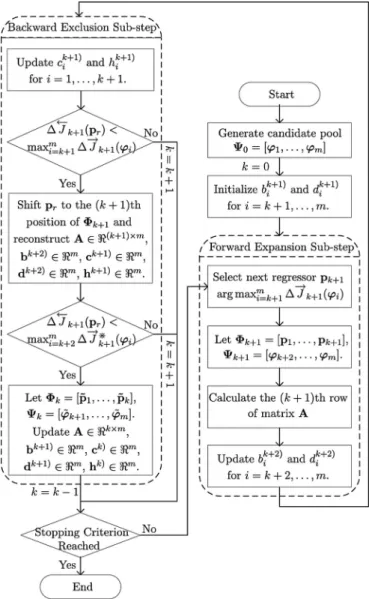
The efficient learning mechanism of the sparse LS-SVM-based fuzzy systems is shown in the flowchart in Fig. 2 and is detailed as follows.
Step 1) Initialization: To start the learning process, the
can-didate pool Ψ0 = [ϕ1, . . . ,ϕm] is first generated by using
all the training patterns as the potential rules/SVs. Note that the initially selected pool Φ0 is an empty matrix. The
num-ber of selected regressors is set to k= 0, and the two vec-tors b1) = [ϕT
1y, . . . ,ϕTmy] and d1) = [ϕT1ϕ1, . . . ,ϕTmϕm]
Fig. 2. Flowchart of the proposed efficient learning mechanism for construct-ing sparse LS-SVM-based fuzzy systems.
Step 2) Forward expansion phase: The main task here is to
select the most significant regressor from the candidate pool and to update the corresponding variables for the operations ahead. 1) According to the contribution of each candidate regressor computed from (30), the one with the largest objective reduction is selected as the next regressor to be added into the regression matrix Φk+ 1 = [p1, . . . ,pk+ 1], i.e.,
pk+ 1 = arg maxmi=k+ 1Δ − →
Jk+ 1(ϕi). The corresponding
regressorpk+ 1 is then removed from the candidate pool
andΨk+ 1 = [ϕk+ 2, . . . ,ϕm]set.
2) The (k+ 1)th row of matrix Ais calculated using (25), while all the previouskrows remain unchanged. 3) The two vectorsbk+ 2)anddk+ 2)are updated with entries
fromk+ 2tomby using (28) and (29) and are employed for selecting the (k+ 2)th regressor from the candidate pool.
Step 3) Backward exclusion phase: The main purpose of this
phase is to reevaluate the contribution of each of the previously selected regressors.
1) The entries from 1 tok+ 1 for the two vectors ck+ 1)
and hk+ 1) are updated using (33) and (34), while the
correspondingly remaining values in the two vectors are inherited frombk+ 2)anddk+ 2).
2) The criterion Δ←−Jk+ 1(pr) = minik= 1Δ←J−k+ 1(pi)<
maxm i=k+ 1Δ
− →J
k+ 1(ϕi)is used to decide whether to
re-move a regressor from the selected pool or not, and to determine which one is to be removed. If the criterion is not met, then setk=k+ 1and go to Step 4. Otherwise, move to the next step.
3) The regressorpris shifted to the last column ofΦk+ 1
us-ing a total ofk−r+ 1interchanges between two adjacent previously selected regressors. Thus, a new regression
context of A∈ (k+ 1)×m, bk+ 2) ∈ m, ck+ 1) ∈ m,
dk+ 2) ∈ m, andhk+ 1) ∈ m is produced as ifp r was
the last selected regressor in the regression matrixΦk+ 1.
4) The criterion Δ←J−k+ 1(pr)<maxmi=k+ 2Δ − →J
k+ 1(ϕi) is
used to decide whether to remove a regressor from the selected pool or not. If none has to be removed, then set k=k+ 1and the algorithm moves to Step 4. Otherwise, go to the next step.
5) The regressorpr is removed from the selected pool and
returned to the candidate pool, i.e., Φk = [p˜1, . . . ,˜pk]
andΨk = [ ˜ϕk+ 1, . . . ,ϕ˜m]. The regression contextA∈ k×m,bk+ 1) ∈ m,ck)∈ m,dk+ 1) ∈ m, andhk) ∈ m are then updated and the indexk is set tok−1 as
described in Section IV-B3.
Step 4) The learning process will terminate if some stopping
criterion is met, such as a certain number of regressors have been selected or some tolerance value has been met. Similar to the stopping criterion commonly used in training neural net-works and SVMs [13], [26], the tolerance for the maximum ratio of objective value reduction is used here. In detail, if the ratio (Jk −minmi=k+ 1Jk+ 1(ϕi))/Jkis less than a very small positive
tolerance value (ρ), the generalization performance of the fuzzy systems will not be greatly improved by adding a new regressor. It should be noted that the stopping criterion used here is an important measure for the tradeoff between the training accu-racy (performance) and the model complexity (sparseness and interpretability) of the obtained fuzzy systems. If the stopping criterion is not met, the algorithm returns to Step 2.
E. Convergence and Computational Complexity
For the convergence, it is obvious that the objective value continuously decreases each time a new regressor is included into the selected pool (i.e., where only the forward expansion phase is applied), with a decrement amount ofΔ−→Jk+ 1(ϕi)at
the(k+ 1)th subset selection step ifϕi(i=k+ 1, . . . , m) is
added as defined in (21) and (30). To reassess the contribution of all the previously selected regressors, the backward exclusion phase is performed to exclude the most insignificant regressor with the smallest contribution to the objective function from the selected pool. Thus, the introduction of this backward exclu-sion phase can cause a small amount of increaseΔ←J−k+ 1(pi)
to the objective value, which is defined in (22) and (35) if a se-lected regressor, saypi(i= 1, . . . , k+ 1), is removed from the
TABLE I
OPERATIONSINVOLVED IN THEPROPOSEDMETHOD
Algorithms/Operations Additions/Subtractions Multiplications/Divisions Total Operations Forward M(N2+N+ 3) + 2N(N−1) M(N2+ 4N+ 2)−M(M+ 1) + 2N2 M(2N 2+ 5N+ 5)−M(M+ 1) + 2N(2N−1) Backward Constant M(N2+N+ 2) +M(M+ 1)/2 + 2N(N−1) M(N2+ 4N+ 1) +M(M+ 1)/2 + 2N2 M(2N2+ 5N+ 3) +M(M+ 1) + 2N(2N−1) Shifting (k−nk+ 1)(2N+ 7) (k−nk+ 1)(2N+ 8) (k−nk+ 1)(4N+ 15) Removing 2N+ 2 3N−1 5N+ 1
selected pool at the (k+ 1)th subset selection step. However, as the criterionmink
i= 1Δ←−Jk+ 1(pi)<maxmi=k+ 1Δ − →J
k+ 1(ϕi)
is used to determine whether or not a regressor is removed and assuming that the objective value on thekth subset selec-tion step at some point isJk, the new objective valueJk
ob-tained after a forward expansion being followed by a backward exclusion is given by Jk=Jk −maxmi=k+ 1Δ
− →J
k+ 1(ϕi) +
mink
i= 1Δ←J−k+ 1(pi)< Jk. Thus, the objective value is reduced
each time a new subset ofkregressors is selected. Obviously, the extreme case is that a nonsparse fuzzy system correspond-ing to the solution of (13) can be obtained if all the regressors are selected as the SVs with a tolerance valueρ= 0. In sum-mary, the convergence of the proposed method composed of iterative forward expansion and backward exclusion phases is guaranteed.
With respect to the computational complexity, the basic arith-metic operations involved in the construction of sparse LS-SVM-based fuzzy systems are additions/subtractions and mul-tiplications/divisions. Assuming that a total ofN data samples are used for training and that a total of M rules have been extracted by the proposed learning mechanism, the number of additions/subtractions and multiplications/divisions and over-all total of operations from only using the forward expansion phase are listed in the first row of Table I. By introducing the backward exclusion phase, the overall computational complex-ity then varies with the different numbers of regressors removed at each selection step and the different position of the removed regressor in the selected pool.
The details of the computational complexity, including both the constant part and the variable part (shifting operations and removing operations), are listed in the last three rows of Table I. The first part constant operations involving (33)–(35) and the forward expansion phase are listed in the second row of Table I. Suppose the forward expansion at the (k+ 1)th step is just com-pleted and a previously selected regressor at thenkth position
inΦk+ 1 is to be removed from current selected pool; then, the
operations involved in shifting this regressor to the last position inΦk+ 1and removing it are given in the third and fourth rows of
Table I. Due to the fact thatN >> M, the computation mainly comes from the term2M N2. In practice, the proposed method
is usually dominated by the forward expansion phase, while the backward exclusion phase works on revising the selected regression pool. Thus, consideringM > k≥nk, the
computa-tional demand of the proposed algorithm does not increase too much, compared with the forward expansion phase. In addition, as described in Section III, it generally needs a computational
complexity ofN3/3 +O(N2)by using the efficient Cholesky
decomposition to solve the KKT system (9) only for nonsparse LS-SVMs. Therefore, the computational advantage of our learn-ing mechanism is significant especially when the trainlearn-ing dataset consists of a larger number of patterns. If the pruning method [25] discussed in Section I is used for imposing the sparseness for the conventional LS-SVM, its computational complexity can also be extremely large. Thus, the computational demand of the proposed learning mechanism in this paper can be dramatically decreased, meanwhile achieving the model sparseness. These will further be demonstrated in the following experimental examples.
V. NUMERICALEXAMPLES
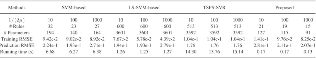
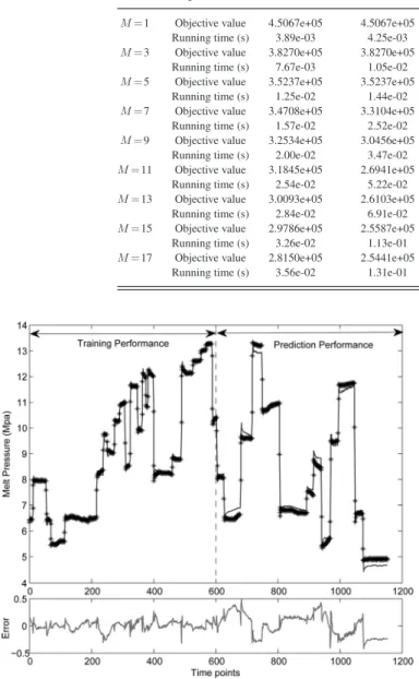
Three simulation and real-world problems are investigated to validate the efficiency and effectiveness of the proposed learning mechanism and the sparseness of LS-SVM-based fuzzy systems constructed. The resulting performances are also compared with other SVM-based fuzzy learning approaches in terms of model sparseness, running time, and model accuracy. The first example is a nonlinear dynamic identification problem [31], the second involves melt pressure prediction in polymer extrusion process [32], and the third is to diagnose the severity of mammographic masses [33]. All the experiments were conducted on an Intel CoreT M2 Duo Processor E8135 2.40 GHz, running the Windows 7 operating system, with programs compiled by MATLAB.
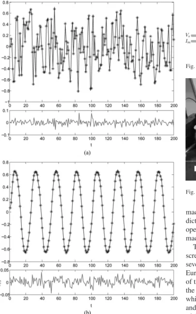
A. Identification of the Nonlinear Dynamic System
The first example [31] involves identifying the following non-linear dynamic system:
y(t) = y(t−1)
1.5 +y2(t−1)−0.3y(t−2) + 0.5u(t−1) +ε(t)
(52) whereε(t)represents a noise sequence [ε(t)∼N(0,0.012)]. A total of 400 simulated data points were then generated. The first 200 samples of training data were obtained by stimulating the system with a random input signalu(t)uniformly distributed in [−1,1], while the remaining 200 samples of test data were pro-duced under using a sinusoidal input signalu(t) = sin(2πt/25). Thus,[u(t−1), y(t−1), y(t−2)]andy(t)constituted the in-put and outin-put variables for the LS-SVM-based fuzzy models to be developed.
The Gaussian widthσwas set to 3, and the regularization pa-rameterμwas set to 1/(2×1000), as is common. To assess the effectiveness of the proposed algorithm in finding better values