A Forecasting Model Based On Combining
Automatic Clustering Technique And Fuzzy
Time Series
Nghiem Van Tinh
Thai Nguyen University of Technology, Thai Nguyen University Thai Nguyen, Vietnam
Abstract—Most fuzzy forecasting methods are
based on modelling fuzzy logical relationships according to the past data. In this paper, a hybrid forecasting model based on two computational approaches, fuzzy logical relationship groups and clustering technique, is presented for forecasting enrolments. Firstly, we use the automatic clustering algorithm to divide the historical data into clusters and adjust them into intervals with different lengths. Then, based on the new obtained intervals, we fuzzify all the historical data into fuzzy sets, define fuzzy logical relationships and calculate the forecasted output value for fuzzy logical relationship groups. To show the effectiveness of the proposed model. We applied the proposed model to forecast the historical enrollments of the University of Alabama. The experimental results show that the proposed method gets a higher average forecasting accuracy rate than the existing methods based on both first – order and high – order fuzzy time series.
Keywords—Fuzzy time series, forecasting, fuzzy logical relationship groups, automatic clustering, enrolments.
I. INTRODUCTION
In our daily life, forecasting activities play an important role. Therefore, many more forecasting models have been developed to deal with various problems in order to help people to make decisions, such as crop forecast [7], [8], academic enrolments [2], [11], the temperature prediction [14], stock markets[15], etc. There is the matter of fact that the traditional forecasting methods cannot deal with the forecasting problems in which the historical data are represented by linguistic values. Ref. [2,3] proposed the time-invariant fuzzy time and the time-variant time series model which use the max–min operations to forecast the enrolments of the University of Alabama. However, the main drawback of these methods is huge computation burden. Then, Ref. [4] proposed the first-order fuzzy time series model by introducing a more efficient arithmetic method. After that, fuzzy time series has been widely studied to improve the accuracy of forecasting in many applications. Ref. [5] considered the trend of the enrolment in the past
years and presented another forecasting model based on the first-order fuzzy time series. Ref. [13] pointed out that the effective length of the intervals in the universe of discourse can affect the forecasting accuracy rate. In other words, the choice of the length of intervals can improve the forecasting results. Ref.[6] presented a
heuristic model for fuzzy forecasting by integrating Chen’s fuzzy forecasting method [4]. At the same time, Ref. [9], [12] proposed several forecast models based on the high-order fuzzy time series to deal with the enrolments forecasting problem. In [9], the length of intervals for the fuzzy time series model was adjusted to get a better forecasted accuracy. Recently, Ref.[17] presented a new hybrid forecasting model which combined particle swarm optimization with fuzzy time series to find proper length of each interval. Ref. [19] presented a method to forecast the Taiwan Stock Exchange Capitalization Weighted Stock Index (TAIEX) based on fuzzy time series and clustering techniques. Additionally, Ref.[18] proposed a new method to forecast enrolments based on automatic clustering techniques and fuzzy logical relationships.
II. FUZZY TIME SERIES AND CLUSTERING ALGORITHM
In this section, we briefly review the basic concepts of fuzzy time series(FTS) and the automatic clustering algorithm.
A. Fuzzy Time Series Definitions
In [2] , Song and Chissom proposed the definition of fuzzy time series based on fuzzy sets ,Let U={u1,u2,…,un } be an universal set; a fuzzy set A of U is defined as A={ fA(u1)/u1+…+fA(un)/un }, where fA is a membership function of a given set A, fA :U [0,1], fA(ui) indicates the grade of membership of ui in the fuzzy set A, fA(ui) ϵ [0, 1], and 1≤ i ≤ n . General definitions of fuzzy time series are given as follows:
Definition 1: Fuzzy time series
Let Y(t) (t = ..., 0, 1, 2 …), a subset of R, be the universe of discourse on which fuzzy sets fi(t) (i =
1,2…) are defined and if F(t) be a collection of fi(t)) (i =
1, 2…). Then, F(t) is called a fuzzy time series on Y(t) (t . . ., 0, 1,2, . . .).
Definition 3: Fuzzy logic relationship
If there exists a fuzzy relationship R(t-1,t), such that F(t) = F(t-1)R(t-1,t), where " " is an arithmetic operator, then F(t) is said to be caused by F(t-1). The relationship between F(t) and F(t-1) can be denoted by F(t-1)→ F(t). Let Ai = F(t) and Aj = F(t-1), the
relationship between F(t) and F(t -1) is denoted by fuzzy logical relationship Ai→ Aj where Ai and Aj refer
to the current state or the left hand side and the next state or the right-hand side of fuzzy time series.
Definition 4: 𝜆- order fuzzy time series
Let F(t) be a fuzzy time series. If F(t) is caused by F(t-1), F(t-2),…, F(t-𝜆+1) F(t-𝜆) then this fuzzy relationship is represented by by F(t-𝜆), …, F(t-2), F(t-1)→ F(t) and is called an 𝝀- order fuzzy time series.
Definition 5: Fuzzy Relationship Groups (FLRGs)
Fuzzy logical relationships in the training datasets with the same fuzzy set on the left-hand-side can be further grouped into a fuzzy logical relationship groups. Suppose there are relationships such that
𝐴𝑖 → 𝐴𝑗 𝐴𝑖 → 𝐴𝑘
…….
So, these fuzzy logical relationships can be grouped into the same FRG as : 𝐴𝑖 → 𝐴𝑗 , 𝐴𝑘…
B. Forecasting Model Based on FTS
The main steps for the FTS forecasting algorithm based on TV-FRGs is shown in the following algorithm
Step 1: Partition the universe of discourse into equally lengthy intervals.
Step 2: Define fuzzy sets on the universe of discourse.
Step 3: Fuzzify all historical data
Step 4: Identify the fuzzy logical relationships
Step 5: Establish the fuzzy logical relationship groups according to Definition 5.
Step 6: Defuzzify and calculate the forecasted output value.
C. An Automatic Clustering Algorithm
In this section, we briefly summarize an automatic clustering algorithm to cluster numerical data into intervals. The algorithm is introduced in [ 20]. The algorithm is composed of the main following steps.
Step 1: Sort the numerical data in an ascending sequence having n different numerical data.
d1, d2, d3, . . . , di, . . . , dn.
where 𝑑1 is the smallest datum among the n numerical data, 𝑑𝑛 is the largest datum among the n numerical data, and 1 ≤ 𝑖 ≤ 𝑛.
Step 2: Put each numerical datum into a cluster, show as follows: {d1}, {d2}, {d3}, . . . , {di}, . . . , {dn}.
Where the symbol ‘‘{ }’’ denotes a cluster, d1 is the smallest datum among the n numerical data, dn is the largest datum among the n numerical data and 1 ≤ i ≤ n.
Step 3: Based on the clustering results obtained in Step 2, adjust these clusters into contiguous intervals
III. FORECASTING MODEL BASED ON AUTOMATIC CLUSTERING ALGORITHM AND FUZZY TIME SERIES
In this section, we present a hybrid method for forecasting enrolments based on the automatic clustering algorithm and fuzzy time series. The historical data of enrolments of the University of Alabama are introduced in article[ ]. The proposed model is now presented as follows:
Step 1: Partition the universe of discourse into n intervals.
In this step, we apply the automatic clustering algorithm [20] to cluster the historical enrolments into clusters and adjust the clusters into 21 intervals with different lengths. Then, calculate the midpoint of each interval as shown in Table 2.
Table 2. The midpoint of each intervals ui (1 ≤ 𝑖 ≤ 21)
No Intervals Midpoint
1 [13055, 13354] 13204.5
2 [13354, 13862] 13608
3 [13862, 14166] 14014
4 [14166, 14397] 14281.5
5 [14397, 14995] 14696
--- --- ----
19 [18876, 18970] 18923
20 [18970, 19328] 19149
21 [19328, 19337] 19332.5
Step 2: Define fuzzy sets Ai, where (1 ≤ 𝑖 ≤ 𝑛)
a fuzzy set Ai (1 ≤ 𝑖 ≤ 21) and its definition is
described in Eq.(1).
Ai = ∑ aij
uj
21 j=1 =
1 if j == i
0.5 if j == i − 1 or j == i + 1
0 otherwise
(1)
where aij∈[0,1], 1 ≤ i ≤ 21, and 1 ≤ j ≤ 21. The
value of aijindicates the grade of membership of uj in
the fuzzy set Ai.
Step 3: Fuzzify variations of the historical enrolment data.
In order to fuzzify all historical data, it’s necessary to assign a corresponding linguistic value to each interval first. The simplest way is to assign the linguistic value with respect to the corresponding fuzzy set that each interval belongs to with the highest membership degree. For example, the historical enrolment of year 1975 is 15460 which falls within u9 =
(15331, 15603], so it belongs to interval u9 Based on
Eq. (1), Since the highest membership degree of u9
occurs at A9, the historical time variable F(1975) is
fuzzified as A9. A complete overview of fuzzified
enrolments is shown Table 3.
Table 3. Fuzzified enrolments of the University of Alabama
Year Actual Fuzzy
set Year Actual
Fuzzy set
1971 13055 A1 1982 15433 A9
1972 13563 A2 1983 15497 A9
1973 13867 A3 1984 15145 A7
1974 14696 A5 1985 15163 A8
1975 15460 A9 1986 15984 A12
1976 15311 A8 1987 16859 A15
1977 15603 A10 1988 18150 A17
1978 15861 A11 1989 18970 A20
1979 16807 A15 1990 19328 A21
1980 16919 A16 1991 19337 A21
1981 16388 A13 1992 18876 A19
Step 4: Identify the fuzzy logical relationships
Relationships are identified from the fuzzified historical data. So, based on Table 3 and according to Definition 2, we get first – order fuzzy logical relationships are shown in Table 4; where the fuzzy logical relationship 𝐴𝑖 → 𝐴𝑘 means "If the enrolment of year i is 𝐴𝑖, then that of year i + 1 is 𝐴𝑘", where 𝐴𝑖 is called the current state of the enrolment, and 𝐴𝑘 is called the next state of the enrolments.
Table 4: The first-order fuzzy logical relationships
𝐴1 −> 𝐴2 ; 𝐴2 −> 𝐴3 ; 𝐴3 −> 𝐴5 ; 𝐴5 −> 𝐴9 ; 𝐴9 −> 𝐴8; 𝐴8 −> 𝐴10; A10 -> A11; A11 -> A15; A15 -> A16; A16 -> A13; A13-> 𝐴9 ; 𝐴9 −> 𝐴9; 𝐴9 −> 𝐴7; 𝐴7 −> 𝐴8 𝐴8 −> 𝐴12 ; 𝐴12 −> A15; A15 -> A17; A17 -> A20; A20 -> A21; A21 -> 𝐴21; 𝐴21 −> 𝐴19
Step 5: Create all FRGs
In [4], all the fuzzy relationship having the same fuzzy set on the left-hand side or the same current state can be put together into one fuzzy relationship group. But, according to the Definition 5, we need to
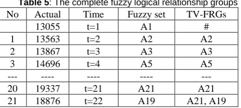
consider the appearance history of the fuzzy sets on the right-hand side too. Therefore, only the fuzz sets on the right hand side appearing before the left-hand side of the relationship group is taken into the same fuzzy logic relationship group. Thus, from Table 4 and based on Definition 5, we can obtain 21 fuzzy logical relationship groups shown in Table 5.
Table 5: The complete fuzzy logical relationship groups
No Actual Time Fuzzy set TV-FRGs
13055 t=1 A1 #
1 13563 t=2 A2 A2
2 13867 t=3 A3 A3
3 14696 t=4 A5 A5
--- ---- ---- ---- ---
20 19337 t=21 A21 A21
21 18876 t=22 A19 A21, A19
Step 6: Defuzzify and calculate the forecasting output value.
Calculate the forecasted output at time t by using the following rules:
Rule 1: If the fuzzified enrolment of year t-1 is Aj
and there is only one fuzzy logical relationship in the fuzzy logical relationship group whose current state is Aj, shown as follows: Aj(t − 1) → Ak(t) , then the
forecasted enrolment of year t is mk, where mk is the
midpoint of the interval uk and the maximum
membership value of the fuzzy set Ak occurs at the
interval uk.
Rule 2: If the fuzzified enrolment of year t -1 is Aj
and there are the following fuzzy logical relationship group whose current state is Aj, shown as follows:
Aj(t − 1) → Ai1(t1), Ai2(t2), Aip(tk)
then the forecasted enrolment of year t is calculated as follows:
forecasted = 1∗ mi1+2∗mi2+3∗mi3+⋯+p∗ mip
1+2+⋯+p
where 𝑚𝑖1, 𝑚𝑖2 , 𝑚𝑖𝑘 are the middle values of the intervals ui1 , ui2 and uip respectively, and the
maximum membership values of Ai1, Ai2 , . . . , Aip occur
at intervals ui1, ui2 , . . . , uip , respectively. From Tables
3 and 5 and based on the Principles in Step 5, we can forecast the enrolments of the University of Alabama from 1971s to 1992s by the proposed method. For example, assume that we want to forecast the enrolment of years 1975 and 1983 are calculated as follows:
[F(t)=F(1975)]. From Table 3, we can see that the fuzzified enrolments of years F(t-1)= F(1974) is A5 .
From Table 5, we can see that there is a fuzzy logical relationship A5(t − 1) → A9(t), in Group 4 and the
maximum membership value of the fuzzy set A9
occurs at the interval u9. Based on rule 1, the
forecasted enrolment of year 1975 can be calculated as follows:
𝐹𝑜𝑟𝑒𝑐𝑎𝑠𝑡𝑒𝑑 = 𝑚9 = 15331+15603
[F(t)=F(1983)]. From Table 3, we can see that the fuzzified enrolments of years F(t-1)= F(1982) is A9 .
From Table 5, we can see that there is a fuzzy logical relationship A9(t − 1) → A8(t1), A9(t); (t1 < t) in
Group 13 and the maximum membership value of the fuzzy set A8 and A9 occurs at the intervals u8 and u9,
respectively. Based on rule 2, the forecasted enrolment of year 1983 can be calculated as follows:
𝐹𝑜𝑟𝑒𝑐𝑎𝑠𝑡𝑒𝑑 =1∗𝑚8+2∗𝑚9
1+2 =
15247+2∗15467
3 =1539.6
Where, 𝑚8=15163+15331
2 = 15247 and 𝑚9 = 15331+15603
2 =15467.
In the same way, we can get the forecasted enrolments of the other years of the University of Alabama from 1971s to 1992s based on the first-order fuzzy time series, as listed in Table 6.
Table 6: Forecasted enrolments of the proposed method
using the first-order FTS.
Year Actual Fuzzified Results 1971 13055 A1 Not forecasted
1972 13563 A2 13608
1973 13867 A3 14014
1974 14696 A5 14696
---- --- ---- ----
1990 19328 A21 19333
1991 19337 A21 19333
1992 18876 A19 19060
To measure the forecasted performance of proposed forecasting method, the mean square error (MSE) is employed as an evaluation criterion to represent the forecasted accuracy. The MSE value is computed as follows:
MSE = 1
n∑ (Fi− Ri) 2 n
i=1 (2)
Where, Ri notes actual data on date i, Fi forecasted value on date i, n is number of the forecasted data
IV. EXPERIMENTAL RESULTS
The performance of the proposed method will be compared with the existing methods, such as the SCI
model [2], the C96 model [4], the H01 model [5],
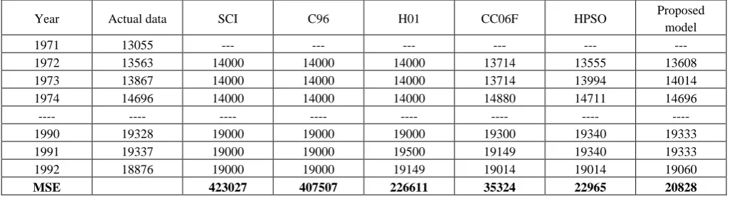
CC06F model [11] and HPSO model [17] based on the enrolment of Alabama University data from 1971 to 1992. The compared results are shown in Table 7.
Table 7: A comparison of the forecasted results of our proposed modelwith the existing models with first-order of the FTS series under different number of intervals
Year Actual data SCI C96 H01 CC06F HPSO Proposed
model
1971 13055 --- --- --- --- --- ---
1972 13563 14000 14000 14000 13714 13555 13608
1973 13867 14000 14000 14000 13714 13994 14014
1974 14696 14000 14000 14000 14880 14711 14696
---- ---- ---- ---- ---- ---- ---- ----
1990 19328 19000 19000 19000 19300 19340 19333
1991 19337 19000 19000 19500 19149 19340 19333
1992 18876 19000 19000 19149 19014 19014 19060
MSE 423027 407507 226611 35324 22965 20828
Table 7 shows a comparison of MSE value according to Eq.(2) of the proposed model based on the first-order fuzzy time series with different number of intervals. The the forecasting accuracy is computed by (3) as follows.
𝑀𝑆𝐸 = ∑𝑛𝑖=1(𝐹𝑖−𝑅𝑖)2
𝑁 =
(13608−13563)2+(14014−13867)2…+(19060−18876)2
21 = 20828
From Table 7, we can see that the proposed method has a smaller MSE value than SCI model [2] the C96
Table 8: A comparison of the MSE of the proposed model with it’s counterparts based on high FTS
Models 3rd- order 4th- order 5th- order 6th- order 7th- order 8th- order
Model [ 21] 208.79 142.26 143.31 147.14 105.02 124.48
Model [17] 152.47 148.14 112.24 122.68 103.61 108.37
Model [22] 70 59.4 57.4 52.2 50.2 57.6
Proposed model 62.6 43.2 41.6 39.5 38.3 40.5
The trend of the curves in Fig.1 indicates the our model is still stable and is close to the actual enrolment of students each year, from 1972s to 1992s for the first-order FTS model.
Furthermore, to demonstrate the effectiveness of the proposed model based on high- order FTS, three forecasting models are presented in articles [17, 21, 22] which are selected to be compared with proposed model. The forecasted errors by MSE value of all models are listed in Table 8.
From Table 8, it is obvious that proposed model significantly outperforms the models [17, 21, 22] based on all orders of fuzzy logical relationships and obtains the smallest MSE value of 38.3 for the 7th-order fuzzy time series.
V. CONCLUSIONS
The fuzzy logical relationships and the lengths of intervals are two critical factors that affect forecasting accuracy of model. In this paper, we have proposed a new forecasting method in the fuzzy time series model based on the fuzzy logical relationship groups and the automatic clustering techniques. In this forecasting model, we tried to classify the historical data of Alabama University into clusters by the automatic clustering techniques and then, adjust the clusters into intervals with different lengths. We apply the proposed method to forecast the enrollments of the University of Alabama using the one-factor first-order fuzzy time series and the one-factor high-order fuzzy time series, respectively. From the experimental results shown in Tables 7-8 and Fig.1, we can see that the proposed method gets higher average forecasting accuracy rates than the existing methods due to the fact that the proposed method gets smaller mean square errors than the existing methods for forecasting the enrollments.
Although this paper shows the superior forecasting capability compared with existing forecasting models; but the proposed model is only tested by the enrolment data. we can apply proposed model to deal with more complicated real-world problems for decision-making such as weather forecast, crop production, stock markets, and etc. That will be the future work of this research.
REFERENCES
[1] J.B. MacQueen, “Some methods for classication and analysis of multivariate observations,” in: Proceedings of the Fifth Symposium on Mathematical Statistics and Probability, vol. 1, University of California Press, Berkeley, CA, pp. 281-297, 1967.
[2] Q. Song, B.S. Chissom, “Forecasting Enrollments with Fuzzy Time Series – Part I,” Fuzzy set and system, vol. 54, pp. 1-9, 1993b.
[3] Q. Song, B.S. Chissom, “Forecasting Enrollments with Fuzzy Time Series – Part II,” Fuzzy set and system, vol. 62, pp. 1-8, 1994.
[4] S.M. Chen, “Forecasting Enrollments based on Fuzzy Time Series,” Fuzzy set and system, vol. 81, pp. 311-319. 1996.
[5] Hwang, J. R., Chen, S. M., & Lee, C. H. Handling forecasting problems using fuzzy time series. Fuzzy Sets and Systems, 100(1–3), 217–228, 1998.
[6] Huarng, K. Heuristic models of fuzzy time series for forecasting. Fuzzy Sets and Systems, 123, 369–386, 2001b .
[7] Singh, S. R. A simple method of forecasting based on fuzzytime series. Applied Mathematics and Computation, 186, 330–339, 2007a.
[8] Singh, S. R. A robust method of forecasting based on fuzzy time series. Applied Mathematics and Computation, 188, 472–484, 2007b.
1972 1974 1976 1978 1980 1982 1984 1986 1988 1990 1992 13,000
14,000 15,000 16,000 17,000 18,000 19,000 20,000
Year
N
um
be
r o
f st
ud
en
ts
[9] S. M. Chen, “Forecasting enrollments based on high-order fuzzy time series”, Cybernetics and Systems: An International Journal, vol. 33, pp. 1-16, 2002.
[10] H.K.. Yu “Weighted fuzzy time series models for TAIEX forecasting ”, Physica A, 349 , pp. 609–624, 2005.
[11] Chen, S.-M., Chung, N.-Y. Forecasting enrollments of students by using fuzzy time series and genetic algorithms. International Journal of Information and Management Sciences 17, 1–17, 2006a.
[12] Chen, S.M., Chung, N.Y. Forecasting enrollments using high-order fuzzy time series and genetic algorithms. International of Intelligent Systems 21, 485–501, 2006b.
[13] Huarng, K. H. Effective lengths of intervals to improve forecasting fuzzy time series. Fuzzy Sets and Systems, 123(3), 387–394, 2001a.
[14] Lee, L.-W., Wang, L.-H., & Chen, S.-M. Temperature prediction and TAIFEX forecasting based on fuzzy logical relationships and genetic algorithms. Expert Systems with Applications, 33, 539–550, 2007.
[15] Jilani, T.A., Burney, S.M.A. A refined fuzzy time series model for stock market forecasting. Physica A 387, 2857– 2862. 2008.
[16] Wang, N.-Y, & Chen, S.-M. Temperature prediction and TAIFEX forecasting based on automatic clustering techniques and two-factors high-order fuzzy time series. Expert Systems with Applications, 36, 2143–2154, 2009.
[17] Kuo, I. H., Horng, S.-J., Kao, T.-W., Lin, T.-L., Lee, C.-L., & Pan. An improved method for forecasting enrollments based on fuzzy time series and particle swarm optimization. Expert Systems with applications, 36, 6108–6117, 2009a.
[18] S.-M. Chen, K. Tanuwijaya, “ Fuzzy forecasting based on high-order fuzzy logical relationships and automatic clustering techniques”, Expert Systems with Applications 38 ,15425–15437, 2011.
[19] Tanuwijaya, K., & Chen, S. M. (2009b). TAIEX forecasting based on fuzzy time series and clustering techniques. In Proceedings of the 2009 international conference on machine learning and cybernetics, Baoding, Hebei, China , pp. 2982–2986, 2009b.
[20] Shyi-Ming Chen, Nai-Yi Wang Jeng-Shyang Pan.
Forecasting enrollments using automatic clustering
techniques and fuzzy logical relationships, Expert Systems with Applications 36 , 11070–11076, 2009.
[21] Lee, L.-W. Wang, L.-H., & Chen, S.-M, “Temperature prediction and TAIFEX forecasting based on hight order fuzzy logical ralationship and genetic simulated annealing techniques,” Expert Systems with Applications, 34, 328– 336, 2008.