Time Series Forecasting Using Hybrid ARIMA and ANN Models Based on DWT Decomposition

(1)

Procedia Computer Science 48 ( 2015 ) 173 – 179

Peer-review under responsibility of scientific committee of International Conference on Computer, Communication and Convergence (ICCC 2015) doi: 10.1016/j.procs.2015.04.167

ScienceDirect

International Conference on Intelligent Computing, Communication & Convergence

(ICCC-2014)

Conference Organized by Interscience Institute of Management and Technology,

Bhubaneswar, Odisha, India

Time Series Forecasting using Hybrid ARIMA and

ANN Models based on DWT Decomposition

Ina Khandelwal*, Ratnadip Adhikari, Ghanshyam Verma

Department of Computer Science and Engineering, The LNM Institute of Information Technology, Jaipur-302031, India

Abstract

Recently Discrete Wavelet Transform (DWT) has led to a tremendous surge in many domains of science and engineering. In this study, we present the advantage of DWT to improve time series forecasting precision. This article suggests a novel technique of forecasting by segregating a time series dataset into linear and nonlinear components through DWT. At first, DWT is used to decompose the in-sample training dataset of the time series into linear (detailed) and non-linear (approximate) parts. Then, the Autoregressive Integrated Moving Average (ARIMA) and Artificial Neural Network (ANN) models are used to separately recognize and predict the reconstructed detailed and approximate components, respectively. In this manner, the proposed approach tactically utilizes the unique strengths of DWT, ARIMA, and ANN to improve the forecasting accuracy. Our hybrid method is tested on four real-world time series and its forecasting results are compared with those of ARIMA, ANN, and Zhang’s

hybrid models. Results clearly show that the proposed method achieves best forecasting accuracies for each series.

Keywords:Time serie forecasting; Discrete wavelet transform; ARIMA model; Artificial neural network; Zhang’s hybrid model

* Corresponding author. Tel.:+91- 9414930740 E-mail address: ina@lnmiit.ac.in

Peer-review under responsibility of scientific committee of International Conference on Computer, Communication and Convergence (ICCC 2015)

(2)

1.Introduction

Time series forecasting is a very active research topic in the domain of science and engineering. The primary objective of time series analysis is to develop a mathematical model that can forecast future observations on the basis of available data. Due to the difficulty in assessing the exact nature of a time series, it is often considerably challenging to generate appropriate forecasts. Over the years, various forecasting models have been developed in literature, of which the Autoregressive Integrated Moving Average (ARIMA) [1] and Artificial Neural Network (ANN) [1, 2] are widely popular. ARIMA models are well-known for their notable forecasting accuracy and flexibility in representing several different types of time series. But, a major limitation is their presumed linear form of the associated data that makes them inappropriate for complex nonlinear time series modeling [1]. ANNs successfully overcome this drawback of ARIMA models, but they have produced mixed results for purely linear time series. This means that neither ARIMA nor ANN is solely sufficient in modeling a real-world time series that almost always contains both linear as well as nonlinear correlation structures [1].

Wavelet transform has been applied in many engineering, signal processing, and statistical problems [3]. It is evident from the previous works that wavelet transform can considerably improve forecasting accuracies [4, 5]. Struzik [4] used wavelet decomposition in forecasting S&P index time series. Hsieh et al. [6] used haar wavelet decomposition for removal of noise from the stock price time series data with the aim to achieve more precise forecasts. Milidiu et al. [7] used haar wavelet together with a clustering algorithm to partition input data into different regions. Choi et al. [8] used a hybrid SARIMA and wavelet transform to forecast the sales time series. Conejo et al. [9] used wavelet transform to decompose electricity price time series and then applied ARIMA to forecast future prices. Wavelet transform has also been used to improve ANN forecasting accuracy [10, 11].

In this study, we propose a hybrid approach that adopts both ARIMA and ANN to adequately model the linear and nonlinear correlation structures of a time series, after a prior decomposition of the series through Discrete Wavelet Transform (DWT). The proposed hybrid method is inspired from a similar concept, pioneered by Zhang [1] who pointed out that a real-world time series generally contains both linear and nonlinear patterns. Our approach accumulates the unique modeling strengths of ARIMA and ANN as well as the decomposition ability of DWT. The proposed method is implemented on four real-world time series and its forecasting accuracy is compared with that of ARIMA, ANN, and Zhang’s hybrid approach in terms of two popular error measures.

The rest of the paper is outlined as follows. The next section describes the ARIMA, ANN, and Zhang’s models. Section 3 presents our proposed hybrid approach. Section 4 reports the empirical results with conclusions in Sec. 5.

2.Time series forecasting models

Over the years, various time series forecasting models have been developed in literature. The random walk, autoregressive (AR), moving average (MA), and ARIMA are some widely recognized statistical forecasting models which predict future observations of a time series on the basis of some linear function of past values and white noise

terms [1, 12]. As such, these models impose the inherent constraint of linearity on the data generating function. To overcome this, various nonlinear models have also been developed in literature. One widely popular among them is ANN that has many salient features [1, 13, 14]. Zhang [1] has rationally combined both ARIMA and ANN models in order to considerably increase the forecasting accuracy.

2.1.ARIMA model

The ARIMA models, pioneered by Box and Jenkins [12] are the most popular and effective statistical models for time series forecasting. These are based on the fundamental principle that the future values of a time series are generated from a linear function of the past observations and white noise terms. An ARIMA(p, d, q) model is mathematically expressed as follows:

1 d

t t

B B y B (1)

(3)

2

1 2

1 q

q

B B B B are the lag polynomials, and B is the lag operator so that Byt yt₁. The constants p, q are the model orders, whereas i

,

j

i

1,2, , ;

p j

1,2, ,

q

are the model parameters. The term

d represents the degree of ordinary differencing, applied to make the series stationary. The appropriate orders of the ARIMA(p, d, q) model are usually determined through the Box-Jenkins model building methodology [1]. Due to the linearity restriction, an ARIMA may not be that effective for modeling a general real-world time series.

2.2.ANN model

ANNs constitute a very successful alternative to the ARIMA models for time series forecasting and have many distinguishing characteristics. One of them is the universal approximation, i.e. an ANN can estimate any nonlinear continuous function up to any desired degree of accuracy [13, 14]. A single hidden layer feedforward ANN with one output node is most commonly used in forecasting applications [1, 2]. A p×q×1ANN has the following output:

0 0 1 1 q p t j j ij t i t j i y g y (2)

Here, _j(j 0,1,2,..., )q , _ij(i 0,1,2,..., ;p j 1,2,..., )q are the weights, ₀, ₀_jare the bias terms, and εt is the white noise. We take the logistic function [1, 13] as the hidden layer activation function g. So far ANNs have been very effective for modeling nonlinearly generated time series, but provided mixed results for linear problems [1].

2.3.Zhang’s hybrid model

Evidently, neither ARIMA nor ANN is universally suitable for all types of time series. This is because almost all real-world time series contains both linear and nonlinear correlation structures among the observations. Zhang [1] has pointed out this important fact and has developed a hybrid approach that applies ARIMA and ANN separately for modeling linear and nonlinear components of a time series. According to Zhang, we have:

t t t

y L N (3)

Where, yt is the observation at time t and Lt, Nt denote linear and nonlinear components, respectively. At first, ARIMA is fitted to the linear component and the corresponding forecast

L

ˆ

_tat time t is obtained. So, the residual at time t is given by

e

t

y L

t

ˆ

t

.

According to Zhang, the residuals dataset after fitting ARIMA contains only

nonlinear component and so can be properly modeled through an ANN. Using p input nodes, the ANN for residuals has the following form: e_t f e_t ₁,e_t ₂, ,e_{t p} _t, where f is a nonlinear function, estimated by the ANN and εt is the white noise. If

N

ˆ

_t is the forecast of this ANN, then the ultimate hybrid forecast at time t is obtained as:

ˆ

_t _t _t

y

L N

(4)

Through empirical analysis with three real-world time series, Zhang has found that his hybrid ARIMA-ANN method has achieved considerably better forecasting accuracies than both ARIMA and ANN models.

3.The proposed DWT based ARIMA-ANN hybrid method

Wavelet transform represents any function as a superimposition of a set of wavelets. As these functions are small waves, located in different times, the wavelet transform can provide crucial information about both time and frequency domains. Mathematically, a DWT can be represented as follows [5, 9, 11]:

2

, ( ) 2 l (2l )

l mt t m (5)

(4)

In this study, we use DWT for obtaining a prior decomposition of a time series into high and low frequency components. The proposed approach consists of two phases, viz. decomposition and reconstruction [8, 15]. In the first phase, the series is decomposed into high (detailed) and low (approximate) pass filters, which respectively pick up the higher and lower frequency components of the series. In the next phase, the high and low frequency components are reconstructed through inverse DWT (IDWT) [5, 8]. After these two phases, an ARIMA is fitted to the reconstructed detailed part and forecasts are generated. Then, an ANN is fitted to the corresponding residuals together with the approximate part. Finally, the combined forecasts are obtained through adding these two component-wise forecasts. Our approach is elaborately presented in Alg. 1.

Algorithm 1. The proposed DWT based hybrid ARIMA-ANN forecasting algorithm

Assumption: Y (original series) = Y(LIN) _{(linear part) +}_Y(NLIN)_{(nonlinear part)}

Inputs: The training dataset _tr _[ ₁_{, , ,}₂ _tr_]T

N

y y y

Y and size Nts of the testing dataset

Outputs: The combined forecast vector Yˆ yˆ_N_tr ₁,yˆ_N_tr ₂, ,yˆ_N_tr _N_ts T Steps:

1. Apply DWT on Ytr to decompose it as follows: [A, D]= DWT(Ytr, ‘filter’)

//AandDare the approximation and details parts, respectively

2. Obtain the reconstructions ap

tr IDWT , ‘filter’

Y A and ds

tr IDWT , ‘filter’

Y D

//It obtains the reconstructed approximation and details parts ofYtr 3. Find the appropriate ARIMA(p, d, q) model for Ytr(ds)

4. Define α=(p+d+q), Neff = Ntr – α, and Yeff = Ytr(ds)( α+1:Ntr) // Yeffis the effective training dataset with sizeNeff 5. Initialize the residual vector R=0(1:Neff) // 0 is the zero vector

6. Initialize YL= 0(1:Ntr+Nts), L= 0(1: (Neff + Nts)), and ts(LIN) = 0(1:Nts) 7. Set YL(1:Ntr)= Ytr(ds)

8. fork=1 to (Neff+Nts) do

9. L(k) = ARIMA ((p, d, q); YL(k:α+k-1)) //Obtain thekth ARIMA forecast through usingYL(k:α+k-1) 10. ifk ≤Neff then 11. R(k) = Yeff(k)– L(k) 12. end if 13. ifk > Ntr then 14. YL(k) = L(k) 15. end if 16. end for

17. ts(LIN) = L(Neff+1:end)

{Estimation of the nonlinear part}

18. Initialize YN= 0(1:Neff+Nts) and ts(NLIN) = 0(1:Nts) 19. Set YN(1:Neff) = R + (Ytr(ap)( α+1:end))

20. Find the appropriate i×h×1 ANN model for YN 21. fork=1 to Ntsdo 22. NLIN ts N eff eff ˆ _k _{ANN , , ;}_{i h}₁ _N _{k i N}_: _k ₁ Y Y //Obtain thek

th_{forecast through}_ANN 23. NLIN N Neff k ˆts k Y Y 24. end for

(5)

0 20 40 60 80 100 0 2000 4000 6000 8000 N um be r of l ynx t ra ppe d 0 200 400 600 1 1.5 2 2.5 E xch an ge r at e (a) (b) 0 50 100 150 200 100 200 300 400 M ont hl y m ini ng da ta 0 50 100 150 200 250 300 0 10 20 30 40 M ont hl y t em pe ra tur e (d) (c) 4.Results

We have conducted experiments with four real-world time series on MATLAB. The ARIMA and ANN models are implemented through the Econometric and Neural Network toolboxes [16], respectively. The model orders are estimated through several in-sample forecasting trials. The series are described in Table 1 and depicted in Fig. 1.

Table 1. Details of the time series datasets

Time series Description Size (total, testing) ARIMA ANN

Lynx Annual number of lynx trapped in Mackenzie river district (1821–1934) [17] (114, 14) (12, 0, 0) 7×5×1 Exchange rate Weekly exchange rates from British pound to US dollar (1980–1993) [18] (731, 52) (0, 1, 0) 7×6×1 Indian mining Monthly mining data of India (April, 1981–March, 1998) [19] (204, 30) (13, 0, 0) 12×9×1 US temperature Average monthly temperature of Las Vegas, US (June, 1986–May, 2011) [17] (300, 60) (12, 0, 0) 12×6×1

Fig. 1. The time plots of the series: (a) Lynx, (b) Exchange rate, (c) Indian mining, (d) US temperature From the earlier works, it is evident that the haar and daubechies wavelets are most commonly used for forecasting applications [5, 6, 7]. To mitigate the problem of selecting the appropriate wavelet, in this study, we take the average of the forecasts through three wavelet transforms, viz. harr, db2, and db4. Table 2 presents the obtained forecasting

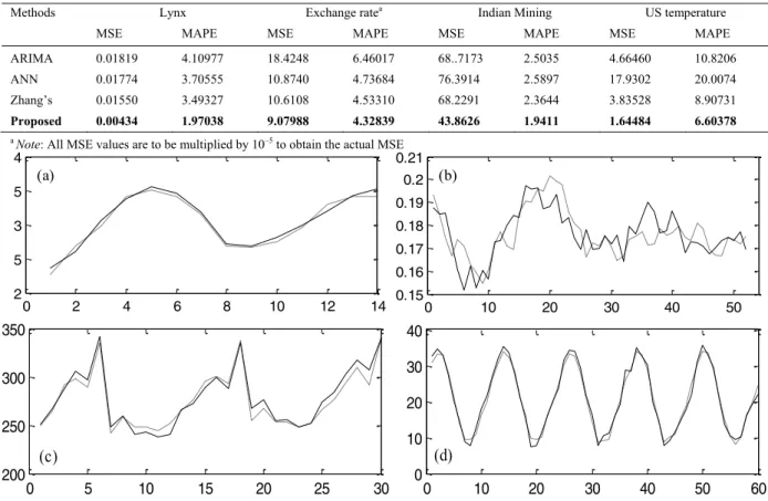
results through ARIMA, ANN, Zhang’s model, and the proposed hybrid method in terms of Mean Squared Error (MSE) and Mean Absolute Percentage Error (MAPE) [1, 14, 20]. From Table 2, it can be clearly seen that Zhang’s

model has achieved lower errors than both ARIMA and ANN and that our DWT based hybrid approach has outperformed all the three models through producing least errors. Figure 2 depicts the actual testing dataset (solid line) and its forecast (dotted line) through the proposed hybrid method for all four time series.

5.Conclusions

Achieving reasonably accurate forecasts of a time series is a very important yet challenging task. ARIMA and ANN are two widely popular and effective forecasting models. ARIMA assumes linear data generations function, whereas ANN is most suitable for nonlinearly generated time series. But, it is almost impossible to establish the exact nature of a series and a real-world time series most often contains both linear as well as nonlinear correlation structures. As such, in this paper, we have proposed a hybrid forecasting method that applies ARIMA and ANN separately to model linear and nonlinear components, respectively after a prior decomposition of the series into low

(6)

0 5 10 15 20 25 30 200 250 300 350 0 10 20 30 40 50 60 0 10 20 30 40 (d) (c)

and high frequency signals through DWT. The final combined forecasts are obtained as the averages of the forecasts through harr, db2, and db4 wavelets. The empirical results with four real-world time series clearly demonstrate that

the proposed method has yielded notably better forecasts than ARIMA, ANN, and Zhang’s hybrid model.

Table 2. The obtained forecasting results

Methods Lynx Exchange ratea _{Indian Mining} _{US temperature}

MSE MAPE MSE MAPE MSE MAPE MSE MAPE

ARIMA 0.01819 4.10977 18.4248 6.46017 68..7173 2.5035 4.66460 10.8206

ANN 0.01774 3.70555 10.8740 4.73684 76.3914 2.5897 17.9302 20.0074 Zhang’s 0.01550 3.49327 10.6108 4.53310 68.2291 2.3644 3.83528 8.90731

Proposed 0.00434 1.97038 9.07988 4.32839 43.8626 1.9411 1.64484 6.60378

a _Note_{: All MSE values are to be multiplied by 10}–5_{to obtain the actual MSE}

Fig. 2. Testing set and its forecast through the proposed method for: (a) Lynx, (b) Exchange rate, (c) Indian mining, (d) US temperature References

1. Zhang, G.,P. (2003). Time series forecasting using a hybrid ARIMA and neural network model. Neurocomputing 50, 159-175.

2. Zhang, G. P., Qi, M. (2005). Neural network forecasting for seasonal and trend time series. European Journal of Operational Research 160 (2), 501-514.

3. Chaovalit, P., Gangopadhyay, A., Karabatis, G., Chen, Z. (2011). Discrete wavelet transform based time series analysis and mining. ACM Computing surveys. http://doi.acm.org/10.1145/1883612.1883613. 43 (2), 0360-0300.

4. Struzik, Z. R. (2001): Wavelet methods in (financial) time-series processing. Physica A: Statistical Mechanics and its Applications 296 (1), 307-319. 5. Al Wadia, M. T. I. S., Tahir Ismail, M. (2011). Selecting wavelet transforms model in forecasting financial time series data based on ARIMA

model. Applied Mathematical Sciences 5 (7), 315-326.

6. Hsieh, T. J., Hsiao, H. F., Yeh, W. C. (2011). Forecasting stock markets using wavelet transforms and recurrent neural networks: An integrated system based on artificial bee colony algorithm. Applied soft computing 11 (2), 2510-2525.

7. Milidiu, R. L., Machado, R. J., , R. P. (1999). Time-series forecasting through wavelets transformation and a mixture of expert models. Neurocomputing 28 (1), 145-156.

8. Choi, T. M., Yu, Y., Au, K. F. (2011). A hybrid SARIMA wavelet transform method for sales forecasting. Decision Support Systems 51 (1), 130-140. 9. Conejo, A. J., Plazas, M. A., Espinola, R., & Molina, A. B. (2005). Day-ahead electricity price forecasting using the wavelet transform and ARIMA

models. IEEE Transactions on Power Systems 20 (2), 1035-1042.

10. Deka, P. C., Haque, L., Banhatti, A. G. (2012). Discrete wavelet-Ann approach in time series flow forecasting-a case study of Brahmaputra river. International Journal of Earth Sciences and Engineering 5 (4), 673-685.

11. Aussem, A., Murtagh, F. (1997). Combining neural network forecasts on wavelet-transformed time series. Connection Science 9 (1), 113-122.

0 2 4 6 8 10 12 14 2 5 3 5 4 0 10 20 30 40 50 0.15 0.16 0.17 0.18 0.19 0.2 0.21 (a) (b)

(7)

12. Box, G. E. P, Jenkins, G. M. (1970). Time series analysis, forecasting and control. 3rd_{ed. Holden-Day, California.}

13. Zhang, G., Patuwo, B. E., Michael, Y.Hu (1998). Forecasting with artificial neural networks: The state of art. International Journal of Forecasting 14 (1), 35-62.

14. Hamzaçebi, C. (2008). Improving artificial neural networks’ performance in seasonal time series forecasting. Information Sciences 178 (23), 4550-4559.

15. Niu, C., Ji, L. (2012). A hybrid method based on wavelet analysis for short term load forecasting. Journal of Convergence Information Technology 7 (17).

16. Demuth, H., Beale, M., Hagan, M. (2010). Neural network toolbox user's guide. The MathWorks, Natic, MA, USA. 17. Data Market (2014). http://datamarket.com

18. Federal Reserve Bank of St. Louis (2014). http://wikiposit.org/uid?FRED.DEXUSUK 19. Open Government Data Platform, India (2014). http://data.gov.in

20. Adhikari, R., Agrawal, R. K. (2014). A combination of artificial neural network and random walk models for financial time series forecasting. Neural Computing and Applications 24 (6), 1441-1449.