Model Selection Criteria in Multivariate Models with Multiple Structural Changes

H

i-S

ta

t

D

is

cu

ss

io

n

P

a

p

er

Research Unit for Statistical

and Empirical Analysis in Social Sciences (Hi-Stat)

Hi-Stat

Global COE Hi-Stat Discussion Paper Series

June 2010

Model Selection Criteria in Multivariate Models with

Multiple Structural Changes

Eiji Kurozumi

Purevdorj Tuvaandorj

Model Selection Criteria in Multivariate Models with

Multiple Structural Changes

Eiji Kurozumi2 _{Purevdorj Tuvaandorj}

Department of Economics Department of Economics Hitotsubashi University McGill University

May, 2010

Abstract

This paper considers the issue of selecting the number of regressors and the number of structural breaks in multivariate regression models in the possible presence of mul-tiple structural changes. We develop a modified Akaike’s information criterion (AIC), a modified Mallows’ Cp criterion and a modified Bayesian information criterion (BIC). The penalty terms in these criteria are shown to be different from the usual terms. We prove that the modified BIC consistently selects the regressors and the number of breaks whereas the modified AIC and the modified Cp criterion tend to overly choose them with positive probability. The finite sample performance of these criteria is investigated through Monte Carlo simulations and it turns out that our modification is successful in comparison to the classical model selection criteria and the sequential testing procedure with the robust method.

JEL classification: C13; C32

Keywords: structural breaks, AIC; Mallows’ Cp; BIC; information criteria

1_{Correspondence: Eiji Kurozumi, Department of Economics, Hitotsubashi University, 2-1 Naka, Kunitachi,}

Tokyo 186-8601, Japan. E-mail: [email protected]

2

Kurozumi’s research was partially supported by the Ministry of Education, Culture, Sports, Science and Technology under Grants-in-Aid No. 18730142, by the 21st Century Center of Excellence Project and by the Global COE program, the Research Unit for Statistical and Empirical Analysis in Social Sciences at Hitotsubashi University.

1. Introduction

This paper considers the selection of regressors and estimation of the number of structural changes in multivariate regression models in the possible presence of multiple structural changes. Many methods for the selection of regressors have been proposed in the econometric and statistical literature, and it is often the case in practical analyses that the regressors are selected using either testing procedures or model selection criteria. The former methods select the regressors by testing the significance of the coefficients of the regressors and deleting the insignificant coefficients from the models, while the model selection criteria choose the regressors that minimize the given risk functions. The representative model selection criteria in econometric analysis are the Akaike information criterion (AIC) by Akaike (1973), theCp

criterion by Mallows (1973) and the Bayesian information criterion (BIC) by Schwarz (1978) among others. See Burnham and Anderson (2002) and Konishi and Kitagawa (2008) for a general treatment of the model selection criteria.

In addition to the selection of the regressors, we need to consider the possibility of struc-tural changes when we investigate data covering a relatively long sample period. In such a case we usually test for structural changes. Various tests for structural changes have been proposed in the literature, and the most commonly used tests in recent practical analyses are the sup-type test of Andrews (1993) and the exponential and average-type tests of Andrews, Lee and Ploberger (1996) among others. These tests assume the null hypothesis of no changes against the alternative of (multiple) change(s), whereas Bai and Perron (1998) and Bai (1999) proposed tests for the null of` breaks against the alternative of `+ 1 breaks for univariate models. These tests are extended to multivariate models by Qu and Perron (2007), who give a comprehensive treatment on the issue of the estimation, inference, and computation in a system of equations with multiple structural changes. Their treatment is general enough in that less restrictive assumptions are placed on the error term and that models such as vector autoregressions (VAR), seemingly unrelated regressions and panel data models are included in their setup as special cases. See Perron (2006) for a review of the testing and estimation of structural changes.

of breaks. Bai (1997b, 1999), Bai and Perron (1998) and Qu and Perron (2007) proposed to implement tests for structural changes sequentially and proved that the estimated number of structural changes is consistent by letting the significance level go to zero. Alternatively, in the statistical literature, the model selection criteria have been proposed to select the number of breaks. For independent normal random variables with mean shifts, Yao (1988) and Zhang and Siegmund (2007) derived the modified BIC and Ninomiya (2005) proposed to modify the AIC, while Liu, Wu and Zidek (1997) considered the modified BIC in regression models with i.i.d. regressors. According to these works, the penalty terms of these new criteria are different from those of the corresponding classical criteria because of the irregularity in the change points. Although these results are of interest from a statistical point of view, they cannot be directly applied to economic data because while economic time series variables are typically serially correlated, in the above papers, assumptions such as i.i.d. observations and regressors are made. Exceptions are Ninomiya (2006) and Hansen (2009). The former considered the modified AIC in finite order autoregressive models, but derived under the assumption of known variance. Hansen (2009) established the modified Mallows’Cpcriterion but with only a single break being allowed.

In this paper we develop the model selection criteria in multivariate models allowing lagged dependent variables as regressors in the possible presence of multiple structural changes in both the coefficients and the variance matrices. Our criteria have an advantage over the existing ones in that (i) multivariate models are considered, (ii) serial correlation is taken into account in models by allowing serially correlated regressors, including lagged dependent variables, (iii) structural changes in the variance matrices are allowed. We theatrically derive the AIC,Cp criterion and BIC in models with structural changes and show that the penalty

terms should be modified compared with those of the corresponding classical ones. We confirm by Monte Carlo simulations that this modification of the penalty terms is very important to correctly select the regressors and the number of structural changes in finite samples.

The rest of this paper is organized as follows. We explain the model and assumptions in Section 2. Section 3 establishes the modified AIC, the modifiedCpcriterion and the modified

BIC with multiple structural breaks and discusses the consistency of these criteria. In Section 4, we investigate the finite sample performance of our model selection criteria via simulations.

Concluding remarks are provided in Section 5.

2. Model and Assumptions

Let us consider the followingn-dimensional regression model withmstructural changes (m+1 regimes):

yt= Φjxjt+εt (j= 1,· · ·, m+ 1 and t=Tj−1+ 1,· · ·, Tj) (1)

whereytandxjt aren×1 andpxj×1 vectors of observations, respectively,εtis an error term

and Φj is an n×pxj unknown coefficient matrix in thejth regime. Typically, the regressor xjt includes a constant but trending regressors are not allowed in our model. We use the termpφj = npxj to denote the number of unknown coefficients in each regime, so that the

total number of coefficients is given bypall_φ =Pm+1

j=1 pφj =

Pm+1

j=1 npxj. Similarly, by allowing

structural changes in the variance matrix ofεt, the number of unknown variance components in each regime is pσ = n(n+ 1)/2 and that in all regimes is given by pall_σ = (m+ 1)pσ = (m+ 1)n(n+ 1)/2. We setT0 = 0 andTm+1 =T, so that the total number of observations is

T. In model (1) there arem structural changes (m+ 1 regimes) with change points given by

T1,· · · , Tm. We allow the lagged dependent variables as regressors and in that case, the initial

observations ofyt fort≤0 are assumed to be given. Thus, model (1) includes a VAR model as a special case. Note that the different regressors and the different orders of the lagged dependent variables are allowed depending on the regimes. The main purpose of this paper is to derive the model selection criteria to choose the regressors among the ¯px candidates for regressors and to estimate the number of structural changesm. In what follows, while we will continue using “choose the numberpx among the ¯px regressors,” we, however, imply “choose

the regressorsx1t, x2t,· · · , xm+1tfor all the regimes among the ¯px candidates for regressors.”

Model (1) can be rewritten asyt= (x0jt⊗In)φj+εtfor thejth regime whereφj = vec(Φj)

is apφj×1 vector. We denote the true value of a parameter with superscript 0. For example, φ0_j and T_j0 denote the true value of φj in the jth regime and the true jth break point, respectively. Hence, the data generating process is given by

The following assumptions are supposed mainly for the derivation of the modified AIC and the modifiedCp criterion.

Assumption A1 (a) There exists a positive integer l0 > 0 such that for all l > l0, the

minimum eigenvalues of (1/l)PT 0 j−1+l t=T0 j−1+1 xjtx0jt and (1/l) PT 0 j t=T0 j−l

xjtx0jt are bounded away

from zero (j= 1,· · ·, m0+ 1). (b)Pl

t=kxjtx

0

jt is invertible for l−k > k0 for some 0< k0 <

∞. (c) sup_j,tEkxjtk4+δ_{<∞ for someδ >0.}

Assumption A2 When the lagged dependent variables are allowed as regressors, all the characteristic roots associated with the lag polynomials are inside the unit circle.

Assumption A3 (a) εt = (Σ0j)1/2ηt for Tj0−1 + 1 ≤ t ≤ Tj0 (j = 1,· · ·, m0 + 1), where

Σ0_j is a symmetric and positive definite unknown matrix and {ηt} is a martingale

differ-ence sequdiffer-ence with respect to Ft = σ{ηt, ηt−1,· · ·, zt+1, zt,· · · ,} with E[ηtη0t|Ft−1] = In for

all t. (b) sup_tEkηtk4+δ _{< ∞ for some δ > 0. (c) E[ηitηjtηkt] = 0 (i, j, k = 1,· · · , n).}

(d) (1/∆T_j0)tr ( PT 0 j t=T0 j−1+1 (ηtη_t0−In) 2) p

−→ κ4j, where κ4 is some positive number and

∆T_j0 =T_j0−T_j0₋₁ (j= 1,· · ·, m0+ 1).

Assumption A4 φ0_j+1 −φ0_j = vTδj and Σ0_j+1 −Σ0_j = vTΨj, where (δj,Ψj) 6= 0 (j =

1,· · · , m0_{), Σ}0

j →Σ0 as T → ∞ for allj andvT is a sequence of positive numbers such that vT →0 and

√

T vT/(logT)2→ ∞.

Assumption A5 0 =λ0 < λ01< ... < λ0m0 < λm0₊₁= 1, whereT_j0 = [T λ0_j](j = 0,· · · , m0+

1).

Assumption A6 The following weak law of large numbers and the functional central limit theorems hold (j= 1,· · ·, m0): 1 ∆T_j0 T0 j X t=T0 j−1+1 xjtx0_jt⊗(Σ0_j)−1−→p Q1j, 1 ∆T_j0₊₁ T0 j+1 X t=T0 j+1 xj+1tx0j+1t⊗(Σ0j+1) −1 p −→Q2j, vT T0 j X t=T0 j−[vv −2 T ] (ηtη0t−In)⇒ξ1j(v), vT T0 j+[vv −2 T ] X t=T0 j+1 (ηtηt0−In)⇒ξ2j(v),

vT Tj0 X t=T0 j−[vv −2 T ] xjt⊗(Σ0j)−1/2 ηt⇒Q11/j2ζ1j(v), vT Tj0+[vv −2 T ] X t=T0 j+1 xj+1t⊗(Σ0j+1)−1/2 ηt⇒Q12/j2ζ2j(v)

for v ≥ 0, where Q1j and Q2j are positive definite matrices, p

−→ and ⇒ signify conver-gence in probability and weak converconver-gence of the associated probability measures, respectively, each entry of ξ1j(v) and ξ2j(v) is a (nonstandard) Brownian motion process on [0,∞) with V ar(vec(ξ1j(1)) = Ω1j and V ar(vec(ξ2j(1)) = Ω2j, while each element of ζ1j(v) and ζ2j(v)

is a standard Brownian motion process on [0,∞), and ξ1j(v), ξ2j(v), ζ1j(v) and ζ2j(v) are

independent of each other.

The above assumptions satisfy or are similar to the conditions provided by the existing literature. For detailed explanations, see Bai (1997a) and Bai and Perron (1998) for the univariate case and Bai (2000) and Qu and Perron (2007) for the multivariate case. Note that we do not allow serial correlation in the error term to derive the model selection criteria. This is more restrictive as compared to the assumptions in Qu and Perron (2007). However, since the lagged dependent variables are allowed as regressors and some elements ofxjt can

be the lagged values of the other elements, Assumption A3 may not be too restrictive for practical purposes. We should also note that the regressorxjt is not necessarily homogeneous in all the regimes. In other words, the regime-wise heteroskedastic regressors are allowed in our model. It is known that the assumption of heteroskedasticity in xjt and the shrinking

shifts in Assumption A4 result in the asymmetric limiting distributions of the break point estimators. This asymmetry will make the modified AIC and the modifiedCp criterion take relatively complicated forms.

We estimate model (1) by the quasi-maximum likelihood (QML) method, conditional on the initial values if the lagged dependent variables are allowed as regressors. Let φ = [φ0₁, φ0₂,· · · , φ0_m+1]0,σ = [vec(Σ1)0,vec(Σ2)0,· · · ,vec(Σm+1)0]0,θ= [φ0, σ0]0andT = [T1, T2,· · ·, Tm]0.

Then, given the number of breaks and the regressors, the log-likelihood function, denoted by

`m,px(T, θ|y, x), becomes `m,px(T, θ|y, x) = − nT 2 log 2π− m+1 X j=1 ∆Tj 2 log|Σj|

−1 2 m+1 X j=1 Tj X t=Tj−1+1 {yt−(x0jt⊗In)φj}0Σj−1{yt−(x0jt⊗In)φj}, (2)

where ∆Tj =Tj −Tj−1 and the subscripts m and px signify that the log-likelihood function

depends on the number of structural changes and the selected regressors, respectively. The maximum likelihood estimators (MLE) of θ and T for given m and px are obtained by maximizing (2) over{(λ1,· · ·, λm); |λj+1−λj| ≥ for j = 1,· · · , m} for small >0 and

are denoted by ˆθ and ˆT, respectively.

Under Assumptions A1-A6, Qu and Perron (2007) showed that the MLEs ofφj and Σj

have the standard asymptotic distributions as in the case of known break points, whereas the limiting distributions of the break date estimators are given by, forj= 1,· · ·, m0,

v2_T( ˆTj −T_j0)−→d argmax

v

B_jI(v) (3)

where the superscriptI denotes the dependency on the indicator function given byI(v≤0),

B_jI(v) = ( B1j(v) = √ ω1jW1j(|v|)−|v₂|γ1j : v≤0 B2j(v) = √ ω2jW2j(v)−v₂γ2j : v >0, (4) ω1j = 1 4vec(A1j) 0_Ω 1jvec(A1j)+δj0Q1jδj, γ1j = 1 2tr(A 2 1j)+δj0Q1jδj, A1j = (Σj0)−1/2Ψj(Σ0j)−1/2, ω2j = 1 4vec(A2j) 0 Ω2jvec(A2j)+δj0Q2jδj, γ2j = 1 2tr(A 2 2j)+δ 0 jQ2jδj, A2j = (Σ0j+1) −1/2_Ψ j(Σ0j+1) −1/2_,

andW1j(v) andW2j(v) are independent standard Brownian motions on [0,∞).

Before moving to the derivation of the model selection criteria, we give the following lemma.

Lemma 1 Let B_jI(v) be defined as in (4). Then,

Ehmax v B I j(v) i = r 2 1j+r1jr2j +r22j r1j+r2j , (5) E aI_j argmax v B_jI(v) = 2 ( a2 γ2j _r2 2j(2r1j+r2j) (r1j+r2j)2 + a1 γ1j _r2 1j(r1j+ 2r2j) (r1j+r2j)2 ) , (6) E aI_jargmax v Bj(v) = 2 ( a2 γ2j _r2 2j(2r1j+r2j) (r1j+r2j)2 − a1 γ1j _r2 1j(r1j+ 2r2j) (r1j+r2j)2 ) , (7)

Although the above three expectations are generally expressed using complicated forms, they can be written in a simpler manner in special cases. For example, whena1 =γ1j and a2 =γ2j, (6) and (7) become E aI_j argmax v BI_j(v) = 2r 2 1j+r1jr2j+r22j r1j+r2j , E aI_jargmax v B_jI(v) = 2(r2j−r1j)(r 2 1j+ 3r1jr2j+r22j) (r1j+r2j)2 .

In addition, ifxjt is homoskedastic across the regimes, BIj(v) has a symmetric distribution

withω1j =ω2j =ωj and γ1j =γ2j =γj so that the expectations reduce to

Ehmax v B I j(v) i = 3 2rj, E aI_j argmax v B_jI(v) = 3rj, E aI_jargmax v B_jI(v) = 0,

whererj =r1j =r2j. Moreover, if r1j =r2j = 1 as in the case of the Gaussian error, then

we have Ehmax v B I j(v) i = 3 2, E aI_j argmax v B_jI(v) = 3, E aI_jargmax v B_jI(v) = 0,

which are the same as obtained in Ninomiya (2005). Lemma 1 will be used to derive the modified AIC and the modifiedCp criterion in the next section.

3. Derivation of Model Selection Criteria

In this section we derive the three model selection criteria, AIC,Cpcriterion and BIC, taking

structural changes into account. More precisely, let ¯px and ¯mbe the largest number of

regres-sors and the largest number of structural changes, respectively, which we have to prespecify. We propose to choose px and m among the ¯px candidates for regressors and 0 ≤ m ≤ m¯, respectively, based on the derived model selection criteria, where though we conventionally state “choose px,” we imply that we select an optimal set of regressors x1t, x2t,· · ·, xm+1t

among the ¯px candidates. Note that all of the following three criteria are designed to choose the model that minimizes them.

Akaike information criterion (AIC) is defined as the unbiased estimator of (−2) times the expected log-likelihood given by Ey[Ey∗[`m,p

x( ˆT,θˆ|y

∗_{, x}∗_{)]], which is in turn equivalent to 2}

times the Kullback-Leibler (KL) information, wherey∗andx∗have the same distribution asy

andxbut are independent ofyandx, andEy andEy∗ are expectation operators with respect toy and y∗, respectively. See, for example, Burnham and Anderson (2002) and Konishi and Kitagawa (2008). Note that ˆT and ˆθ are based not on y∗ but on y. Since we choose the model that minimizes the AIC, we can interpret the chosen model as optimal in the sense that it minimizes the KL information.

Akaike (1973) proposed to estimate the expected likelihood by the empirical log-likelihood but he also showed that the empirical log-log-likelihood is the biased estimator of the expected log-likelihood in finite samples. As in Akaike (1973) we consider the following criterion that depends on the number of structural changes m and the selected regressors, which we conventionally denote aspx:

AIC(m, px) =−2`m,px( ˆT,θˆ|y, x) + 2bm,px( ˆT,θˆ), (8)

where bm,px( ˆT,θˆ) = Ey[`m,px( ˆT,θˆ|y, x) −Ey∗[`m,px( ˆT,θˆ|y

∗_{, x}∗_{)]] corresponds to the bias.}

Since the first term on the right hand side of (8) is the maximized log-likelihood obtained by the QML estimation, we only need to evaluate the bias term explicitly.

In order to calculate the bias, we decomposebm,px( ˆT,θˆ) into four parts as follows:

bm,px( ˆT,θˆ) = Ey h `m,px( ˆT,θˆ|y, x)−Ey∗ h `m,px( ˆT,θˆ|y ∗_{, x}∗₎ii = Ey h `m,px( ˆT,θˆ|y, x)−`m,px(T 0_{, θ}0_{|y, x)}i +Ey`m,px(T 0<sub>, θ</sub>0<sub>|y, x)−Ey∗</sub> `m,px(T 0_{, θ}0_|y∗ , x∗) +Ey h Ey∗`m,p x(T 0<sub>, θ</sub>0<sub>|y</sub>∗ , x∗)−Ey∗ h `m,px(T 0_,θˆ|y∗ , x∗) ii +Ey h Ey∗ h `m,px(T 0<sub>,θˆ|y</sub>∗<sub>, x</sub>∗<sub>)</sub>i<sub>−E</sub> y∗ h `m,px( ˆT,θˆ|y ∗_{, x}∗₎ii = bm,px,1+bm,px,2+bm,px,3+bm,px,4, say. (9)

As in the literature we evaluatebm,px,1 tobm,px,4 up to theO(1) terms for the true values

Proposition 1 Under Assumptions A1-A6 withm=m0 andpx=p0x, the bias termsbm,px,1, bm,px,2, bm,px,3 and bm,px,4 are, up to the O(1) terms, given by

bm,px,1 = pall_φ 2 + m+1 X j=1 κ4j 4 + m X j=1 r₁2_j+r1jr2j+r22j r1j+r2j , bm,px,2 = 0, bm,px,3 = m+1 X j=1 κ4j 4 + pall_φ 2 , bm,px,4= m X j=1 r₁2_j+r1jr2j+r₂2_j r1j+r2j .

Proposition 1 suggests that the modified AIC should be defined as

M AIC(m, px) =−2`m,px( ˆT,θˆ|y, x) + 2p all φ + m+1 X j=1 ˆ κ4j + 4 m X j=1 ˆ r₁2_j+ ˆr1jˆr2j + ˆr22j ˆ r1j+ ˆr2j , (10)

where ˆ denotes the consistent estimator of the corresponding parameter. The estimators of the parameters are given by ˆκ4j = tr( ˆΩj),

ˆ r1j = 1 4vec( ˆA1j) 0_Ωˆ jvec( ˆA1j) + ˆδ_j0Qˆ1jδjˆ 1 2tr( ˆA21j) + ˆδ0jQˆ1jδˆj , and rˆ2j = 1 4vec( ˆA2j) 0_Ωˆ j+1vec( ˆA2j) + ˆδ_j0Qˆ2jˆδj 1 2tr( ˆA22j) + ˆδj0Qˆ2jδˆj , where Ωˆj = 1 ∆ ˆTj ˆ Tj X t= ˆTj−1+1 vec(ˆηtηˆ0t−In)vec(ˆηtηˆ0t−In)0, δˆj = ˆφj+1−φˆj, ˆ A1j = ˆΣ −1/2 j ˆ Σj+1−Σˆj ˆ Σ−_j1/2, Aˆ2j = ˆΣ −1/2 j+1 ˆ Σj+1−Σˆj ˆ Σ−_j+11/2, Σˆj = 1 ∆ ˆTj ˆ Tj X t= ˆTj−1+1 ˆ εtεˆ0_t ˆ Q1j = 1 ∆ ˆTj ˆ Tj X t= ˆTj−1+1 (xjtx0jt⊗Σˆj−1) and Qˆ2j = 1 ∆ ˆTj+1 ˆ Tj+1 X t= ˆTj+1 (xjtx0jt⊗Σˆ−j+11 ) with ˆεt=yt−(x0jt⊗In) ˆφj for ˆTj−1+ 1≤t≤Tˆj (j= 1,· · ·, m).

Although (10) is expressed in a complicated form, the modified AIC can be simplified in several interesting cases. For example, when there are no weakly exogenous regressors and model (1) is a pure VAR model, the limiting distributions of the break point estimators are symmetric with ω1j =ω2j =ωj and γ1j = γ2j = γj as shown by Bai (2000). In this case, r1j =r2j =rj so that M AIC(m, px) =−2`m,px( ˆT,θˆ|y, x) + 2p all φ + m+1 X j=1 ˆ κ4j + 6 m X j=1 ˆ rj.

When ηt is Gaussian, it can be shown that κ4j = n(n+ 1) = 2pσ for all j. In

ad-dition, we have ω1j = γ1j and ω2j = γ2j because vec(A1j)0Ω1jvec(A1j)/2 = tr(A2_1j) and

vec(A2j)0Ω2jvec(A2j)/2 = tr(A22j) as shown in Remark 5 of Qu and Perron (2007). As a

result,r1j =r2j = 1 so that the modified AIC reduces to

M AIC(m, px) =−2`m,px( ˆT,θˆ|y, x) + 2(p all

φ +pallσ ) + 6m. (11)

Even if ηt is not Gaussian but if there are no changes in the variance matrices, the

modified AIC takes a simple form. In this case, BI_j(s) becomes as given by (4) with ω1j = γ1j =δj0Q1jδ1j and ω2j =γ2j =δ0jQ2jδj. Again, we have r1j =r2j = 1, so that the modified

AIC reduces to

M AIC(m, px) =−2`m,px( ˆT,θˆ|y, x) + 2p all

φ + 6m (12)

where we omitκ4 because this term is common for all the models in this case.

In any case we can see that the penalty term of the modified AIC is different from the classical one, which is 2 times the number of unknown coefficients given by 2pall_φ . In order to see the intuitive meaning of the penalty term of the modified AIC, we first consider the case where m is prefixed and one additional regressor is included in each regime. In this case, the third and fourth terms on the right hand side of (10) are basically the same except for the changes in the estimators of κ4j, r1j and r2j while the second term is increased by

2(m+ 1)nbecause the difference between the number of unknown coefficients in the two cases is 2Pm+1

j=1 n(pxj+ 1)−2

Pm+1

j=1 npxj = 2(m+ 1)n. Since (m+ 1)nis the number of additional

unknown coefficients, the penalty on the additional regressors is the same as in the classical case.

Next, let us consider the case where the number of structural changes is increased from

m−1 tom. For ease of exposition, consider the case where the additional break is found in the last regime withpxm+1 regressors. From (10) the penalty term is increased by

2 pxm+1+ ˆ κ4,m+1 2 + 2 ˆ r₁2_m+ ˆr1mrˆ2m+ ˆr22m ˆ r1m+ ˆr2m . (13)

The first term in the parentheses of (13) is interpreted as the penalty on the additional regressors, while the second term corresponds to the penalty on the increased number of

unknown variance components. That is, when the number of structural changes increases, we need to estimate the variance matrix in the additional new regime given by Σm+1 and

ˆ

κ4,m+1/2 can be interpreted as the penalty on Σm+1. In fact, whenηt is Gaussian,κ4,m+1/2

becomes equal ton(n+ 1)/2, which is the same as the number of unknown components,pσ,

in Σm+1.

On the other hand, the third term in the parentheses of (13) can be interpreted as the penalty on searching for an additional break because this term does not appear when the

mth break point, T_m0, is known but does appear when we estimate it, as is understood from the proof of Proposition 1. When we estimate the additional unknown break, we look for the break point that maximizes the log-likelihood; further, the maximizing point is not necessarily the true break date. In general, the maximization is possibly attained at a point different from the true break date in finite samples. In other words, the uncertainty of the break point always leads to a larger log-likelihood (or a smaller model selection criterion) and the third term of (13) can be interpreted as the penalty on this uncertainty. In fact, we can see from (3) and Lemma 1 that the third term in the parentheses of (13) is an approximation of E[γ_jIv_T2|Tmˆ −T_m0|], which can be seen as a measure of the uncertainty of the mth break point, whereγ_jI =γ1j for v ≤0 and γjI =γ2j forv >0. Thus, the more uncertain or more

volatile the break point estimator, the heavier the penalty imposed on the modified criterion. As is seen in (11) and (12), this penalty becomes equal to 6 (= 2×3) in special cases such as when the error is Gaussian and when there are no breaks in the variance matrix, because

E[γI_jv2_T|Tmˆ −T_m0|] = 3 in these cases. We also note that the third term of (13) is an increasing function of r1j = ω1j/γ1j and r2j = ω2j/γ2j, both of which become larger when the break

point estimator is more volatile (for largerω1j andω2j). Since this penalty on the uncertainty

is positive, the modified AIC will choose a smaller number of structural changes than the classical AIC. This property will be confirmed by the simulations in a later section.

3.2. Mallows’ Cp criterion

Mallows (1973) focused on the prediction of the conditional mean of a univariate model and proposed as a measure of adequacy for prediction the scaled sum of squared forecast errors. In this subsection we extend the Mallows’Cp criterion to multivariate models with multiple

structural changes by introducing a multivariate version of the scaled sum of square forecast errors. The model minimizing the modifiedCp criterion is optimal from the viewpoint of the minimization of the risk function based on the forecast errors.

Let µ0_t = (x0_jt⊗In)φ0_j be the conditional mean of yt for T_j0₋₁ + 1 ≤ t ≤ T_j0 and ˆµt = (x0_jt ⊗In) ˆφj be its estimator for ˆTj−1 + 1 ≤ t ≤ Tˆj (j = 1,· · · , m+ 1). As suggested by

Mallows (1973) we adopt as a measure of adequacy of prediction the trace of the scaled residual variance matrix given by

Jm,px = m+1 X j=1 tr   Σ 0−1 j T0 j X t=T0 j−1+1 ˆ µt−µ0_t µtˆ −µ0_t0   .

Let ˆεt=yt−µˆtfor ˆTj−1+1≤t≤Tˆjas defined before and ˜εt=yt−µ˜twith ˜µt= (x0jt⊗In) ˆφj

for T_j0₋₁+ 1 ≤ t ≤ T_j0. That is, ˆεt is the residual from the ML estimation while ˜εt is the

residual when we forecast the conditional mean by (xjt⊗In) ˆφj in the true regimes. Since

yt=µ0_t+εt= ˆµt+ ˆεt= ˜µt+ ˜εt,Jm,px becomes Jm,px = m+1 X j=1 Tj0 X t=T0 j−1+1 (εt−εˆt)0Σj0−1(εt−εˆt) = m+1 X j=1 T0 j X t=T0 j−1+1 ε0_tΣ0_j−1εt−2 m+1 X j=1 T0 j X t=T0 j−1+1 (yt−µˆt)0Σ0j−1εt+ m+1 X j=1 T0 j X t=T0 j−1+1 ˆ ε0_tΣ0_j−1εˆt = − m+1 X j=1 T0 j X t=T0 j−1+1 ε0_tΣ0_j−1εt+ 2 m+1 X j=1 T0 j X t=T0 j−1+1 (ˆµt−µ0t) 0_Σ0−1 j εt − m+1 X j=1    ˆ Tj X t= ˆTj−1+1 ˆ ε0_tΣ0_j−1εˆt− T0 j X t=T0 j−1+1 ˆ ε0_tΣ0_j−1εˆt   + m+1 X j=1 ˆ Tj X t= ˆTj−1+1 ˆ ε0_tΣ0_j−1εˆt = Jm,px,1+Jm,px,2+Jm,px,3+ m+1 X j=1 ˆ Tj X t= ˆTj−1+1 ˆ ε0_tΣ0_j−1εt,ˆ say. (14)

Following Mallows’ (1973) original work, the modifiedCp criterion is defined as

M Cp(m, px) = m+1 X j=1 ˆ Tj X t= ˆTj−1+1 ˆ ε_t0Σˆ_t,−_m,1_{¯ p¯x}εˆt+E[Jm,px,1+Jm,px,2+Jm,px,3]

where ˆΣt,m,¯ p¯x is the estimator of the variance matrix based on the most general model using m= ¯mandpx= ¯px. For a univariate case (n= 1) with no structural changes, Mallows (1973) showed thatE[Jm,px,1+Jm,px,2+Jm,px,3] = 2px−T and hence the modifiedCp criterion takes

a well known form by ignoring −T. For our model (1) with structural changes, it is easy to see thatE[Jm,px,1] =−nT, which is common for all the models and can be ignored. On the

other hand, it can be shown that the dominant term inJm,px,3 is of orderv

−1

T while Jm,px,2

isOp(1). As can be seen in the proof of Proposition 2 we have

vTJm,px,3 = − m X j=1 1( ˆTj < Tj0)tr(A1j)v2T( ˆTj−Tj0) + 1( ˆTj > Tj0)tr(A2j)v2T( ˆTj−Tj0) +op(1) d −→ − m X j=1 tr(AI_j) argmax v B_jI(v) = ¯Jm,px,3, say, (15)

where AI_j = A1j when v ≤ 0 and AIj = A2j when v > 0. Then, the natural candidate for

the modifiedCp criterion would beM Cp(m, px) =Pm+1

j=1 PTˆj t= ˆTj−1+1εˆ 0 tΣˆ −1 t,m,¯ p¯xεtˆ +E[ ¯Jm,px,3].

However, this criterion may not be informative for the choice of models. For example, when xjt is homoskedastic in all the regimes, argmaxvBjI(v) has a symmetric

distribu-tion, which implies E[ ¯Jm,px,3] = 0. In this case, the modified criterion consists of only

Pm+1 j=1 PTˆj t= ˆTj−1+1εˆ 0 tΣˆ −1

t,m,¯ p¯xεtˆ, which is always minimized when we choose the most general

model.

In order to avoid the above problem we need to evaluate the second dominant term in

Jm,px,3, which would be of the same order as is Jm,px,2. The problem here is that the second

dominant term inJm,px,3will be obtained by the higher order expansion ofv

2

T( ˆTj−Tj0), which

is tedious to derive in practice. We might construct a new criterion by ignoring the whole term ofJm,px,3 but such a criterion may not be optimal from the viewpoint of a measure of

adequacy for prediction.

Because of the above reason, we do not construct the modifiedCpcriterion under Assump-tions A1-A6. Instead, we consider the same criterion under more restrictive assumpAssump-tions; we impose restrictions on the breaks in the variance matrices such that Σ0_j+1−Σ0_j =v_T2Ψj. In

other words, we allow only those breaks that are smaller than the ones supposed in Assump-tion A4. Note that by changing the assumpAssump-tion, the limiting distribuAssump-tions of the break point estimators are not affected by the breaks in the variance matrices but depend only on the

breaks in the coefficients, whereas a measure of prediction given by Jm,px still depends on

the breaks in the variance matrices throughJm,px,3.

Proposition 2 Under Assumptions A1-A6 with Σ0_j+1−Σ0_j =v_T2Ψj and with m = m0 and px=p0x, the expectations of the first three terms ofJm,px are given by, up to the O(1) terms,

E[Jm,px,1] =−nT, E[Jm,px,2] = 2p all φ + 6m, E[Jm,px,3] = 3 2 m X j=1 tr(A1j) γ1j −tr(A2j) γ2j ,

where γ1j =δj0Q1jδj and γ2j =δ0jQ2jδj in this case.

Proposition 2 suggests that the modified Cp criterion should be given by, ignoring the

O(1) terms, M Cp(m, px) = m+1 X j=1 ˆ Tj X t= ˆTj−1+1 ˆ ε0_tΣˆ−_t,m,1_{¯ p¯x}εˆt+ 2pallφ + 6m+ 3 2 m X j=1 tr( ˆA1j) ˆ γ1j − tr( ˆA2j) ˆ γ2j ! . (16)

Note that the last penalty term might be negative depending on the asymmetric property of the limiting distributions of the break point estimators. In the symmetric case the last penalty term disappears so that the modifiedCp criterion reduces to

M Cp(m, px) = m+1 X j=1 ˆ Tj X t= ˆTj−1+1 ˆ ε0_tΣˆ−_t,m,1_{¯ p¯x}εtˆ + 2pall_φ + 6m. (17)

For example, the two sided Brownian motionsBI

j(v) (j= 1,· · · , m0) become symmetric when

there are no structural changes in the variance matrices, when (1) is a pure VAR model and whenxjt is homogeneous across the regimes.

From (16) we can see that the penalty term of the modified Cp criterion is different

from the classical criterion. As in the case of the modified AIC, the second term on the right hand side of (16) is the penalty on the additional regressors while the third term can be interpreted as the penalty on the uncertainty associated with estimating the break points. The last term of (16) is related with the breaks in the variance matrices and the asymmetry of the break point estimators. From the proof of Proposition 2 we can see that the last penalty term is an approximation of −Pm

j=1tr(Aj)E[v2T( ˆTj −Tj0)] where we used

that the additional positive penalty is imposed when Ψj > 0 and E[vT2( ˆTj −Tj0)] < 0 (or

Ψj < 0 and E[v_T2( ˆTj −T_j0)] > 0) and vice versa. To interpret this property, let us assume

that Σ0_j for j = 1,· · ·, m+ 1 are known. In this case, the contribution to Jm,px from

the jth regime should be given by tr[Σ0_j−1PT 0

j t=T0

j−1+1

( ˆµt −µ0t)(ˆµt−µ0t)0] but we need to

replace T_j0 with ˆTj for j = 1,· · · , m in practice. That is, the actual contribution is given

by tr[Σ0_j−1PTˆj

t= ˆTj−1+1( ˆµt

−µ0_t)(ˆµt−µ0_t)0]. In this case, if Ψj > 0, or equivalently, Σ0_j−1 is

larger than Σ0_j−₊₁1 in terms of the matrix, and if ˆTj tends to be smaller than T_j0, then the contribution toJm,px from thejth regime decreases more than expected. In order to adjust

the smaller contribution from thejth regime, we need an additional positive penalty. On the other hand, if, again, Σ0_j−1 is relatively large but if the distribution of ˆTj is skewed to the

right, the contribution to Jm,px from the jth regime is larger than expected and hence we

need to reduce this contribution by a negative penalty. Thus, the last term of (16) can be interpreted as the penalty on the overweight or underweight on the forecast errors caused by the asymmetry of the break point estimators.

We should keep in mind that the modified Cp criterion given by (16) is optimal from

the viewpoint of minimizing the risk function based on the prediction errors only in the case where the magnitude of structural changes in the variance matrices is negligibly small as compared to the magnitude of shifts in the coefficients.

3.3. Bayesian information criterion

Schwarz (1978) considered the problem of model selection in the Bayesian framework, in which a model is selected based on the posterior probability. In this subsection, we derive the modified BIC for models with structural changes using the Laplace approximation technique as explained in Konishi and Kitagawa (2008). The model selected by the modified BIC is optimal from the viewpoint of the maximization of the posterior probability.

LetM(m, px,T) be a model for given m,px and T,P(M(m, px,T)) be the prior

proba-bility of a given model,fM(y|θ, x) be the probability density function (pdf) ofy conditional

posterior probability of modelM(m, px,T) is given by P(M(m, px,T)|y, x) = gM(y|x)P(M(m, px,T)) P gM(y|x)P(M(m, px,T)) , (18)

where the summation is taken by over models M(m, px,T) and gM(y|x) is the marginal

distribution of y conditional on x defined as gM(y|x) = R fM(y|θ, x)πM(θ)dθ. We adopt the model that maximizes the posterior probability (18), but the maximization of (18) is equivalent to the maximization of the numerator on the right hand side of (18) because the denominator is common for all the models. Thus, we consider the maximization of

gM(y|x)P(M(m, px,T)), or equivalently, the minimization of

−2 log{gM(y|x)P(M(m, px,T))}=−2 loggM(y|x)−2 logP(M(m, px,T)). (19)

In order to evaluate (19), we make the following assumptions.

Assumption A7 (a) The conditional pdf of y, fM(y|θ, x), is Gaussian. (b) The priors for φ1,· · ·, φm+1 andΣ−11,· · ·,Σ

−1

m+1are noninformative. (c) The prior probability ofM(m, px,T)

is given byP(M(m, px,T)) =αm,T/Tm where 0< α < αm,T <α <¯ ∞.

Note that we do not have to assume shrinking shifts in the Bayesian framework. Instead, we make assumptions on the priors. Assumption A7 (a) states that we base our analysis on a Gaussian distribution. We can interpret Assumption A7 (b) such that we do not have a priori information on the distributional property of the parameters. Note that the noninformative priors for the reciprocal of the variance matrices are sometimes considered in the Bayesian framework. Assumption A7 (c) is motivated from the following three examples:

• (Example 1) Let us first consider the continuous time framework with 0< t < T. For a given m, letS1, S2,· · · , Sm bem candidates for the break dates that are independently

uniformly distributed on (0, T). Then, the pdf ofSj is 1/T forj = 1,· · · , m. In this case

the break points T1, T2,· · · , Tm correspond to the order statistics S(1), S(2),· · ·, S(m)

whereS(j) is thejth smallest value amongS1, S2,· · ·, Sm. As a result, the joint pdf of

T1, T2,· · · , Tm is given by m!/Tm. This motivates us to assume that for discrete time

and given by m!/Qm

j=1(1−j/T)/Tm. With the assumption that the prior probability

ofmis given by 1/( ¯m+ 1) (the uniform prior form= 0,1,· · · ,m¯), the prior probability of a given model becomes αm,T/Tm whereαm,T ={m!/( ¯m+ 1)}/Qm

j=1(1−j/T).

• (Example 2) Let us again consider the continuous time framework as in Example 1 and suppose that the prior for m is a Poisson process with mean T β where the prior for

β is noninformative (β >0). In this case, the pdf of T1, T2,· · · , Tm conditional on m

is given by m!/Tm (Theorem 2.3.1 in Ross, 1996) and hence the prior probability of a given model becomesR₀∞e−T β(T β)m/m!(m!/Tm)dβ =m!/Tm+1. This motivates us to assume the prior given in Assumption A7 (c) in the discrete time framework.

• (Example 3) Suppose that the probability of the occurrence of structural change at each time is given by a Binomial distribution with parameter ρ, for which the prior is uniform on (0,1). In this case, the prior probability of a given model becomes

R1 0 ρ

m_(1−ρ)m_dρ=m!/Qm

j=1{1−(j−1)/T}/(T+ 1)/Tm, which is of the same form

as in Assumption A7 (c).

Let the MLE of θ = [φ0, σ0]0 for a given set of break points T be ˇθ = [ ˇφ0,σˇ0]0 where ˇ

φ = [ ˇφ1,φˇ2,· · · ,φmˇ +1]0 and ˇσ = [vec( ˇΣ1)0,vec( ˇΣ2)0,· · ·,vec( ˇΣm+1)0]0. Note that ˆθ is the

global MLE withT = ˆT whereas ˇθis obtained for an arbitrary given T. Thus, ˇθis different from ˆθ in general and they are the same only in the case where T = ˆT.

While the second term on the right hand side of (19) is given by 2mlogT −2 logαm,T,

we need to evaluate the first term to obtain the modified BIC.

Proposition 3 Under Assumption A7, the logarithm of the marginal pdf of y given x is expressed as loggM(y|x) =`m,px(T,θˇ|y, x)− m+1 X j=1 pφj+pσ 2 log(Tj−Tj−1) +Op(1). (20) Proposition 3 suggests that, since the second term on the right hand side of (19) is given

by 2mlogT +O(1) from Assumption A7 (c), we should minimize −2 log{gM(y|x)P(M(m, px,T))} = −2`m,px(T,θˇ|y, x) + m+1 X j=1 pφj+pσ log(Tj −Tj−1) + 2mlogT+Op(1).

It is not difficult to see that the first term on the right hand side of the above equation domi-nates the other terms and hence we only have to consider the minimization of−`m,px(T,θˇ|y, x)

as long asT is sufficiently large. Since minT −`m,px(T,θˇ|y, x) =−`m,px( ˆT,θˆ|y, x), we replace

T and ˇθwith the MLEs ˆT and ˆθand propose the following modified BIC:

M BIC1(m, px) =−2`m,px( ˆT,θˆ|y, x) + m+1 X j=1 pφj+pσ log( ˆTj−Tjˆ−1) + 2mlogT. (21)

Since log( ˆTj −Tˆj−1) = logT + log(ˆλj −λˆj−1) = logT +Op(1), we may also simplify the

modified BIC (21) as M BIC2(m, px) =−2`m,px( ˆT,θˆ|y, x) + pall_φ +pall_σ + 2m logT. (22)

It is not difficult to interpret the penalty terms of the two modified BICs. The second term on the right hand side of (21) and (pall_φ +pall_σ ) logT of (22) are the penalty on the additional unknown coefficients and variance components while 2mlogT can be interpreted as the penalty on the uncertainty of the break points.

Since the penalty of the classical BIC on the unknown coefficients is given by pall_φ logT, we can see from (21) thatM BIC1 will tend to choose more regressors than the classical BIC for a givenm ≥1. We also note that the modified BIC (22) takes a form similar to Yao’s (1988) BIC, which is given by

M BICy(m, px) =−2`m,px( ˆT,θˆ|y, x) + (p all

φ +pallσ +m) logT. (23)

On comparing the penalty term, we can see that our modified BIC will tend to choose less number of structural changes than Yao’s BIC.3

3

Yao (1988) obtained the modified BIC by treatingT1, T2,· · ·, Tm as unknown parameters; counting the total number of unknown parameters in the model, which equalspall

φ +pallσ +m; and inserting this number into the formula of the classical BIC. Since we treat the change points in a different way, our modified BIC does not coincide with Yao’s BIC.

3.4. Consistency

In this subsection we investigate whether or not the model selection criteria derived in this paper can choose the appropriate regressors and the true number of structural changes. It is well known that the BIC can consistently choose the true lag length for time series models with no structural changes while the AIC and the Cp criterion tend to choose longer lags than

the true one. See, for example, Shibata (1976), Hannan (1980) and Hannan and Deistler (1988). Thus, we expect that the modified BIC can consistently choose the regressors while the modified AIC and the modified Cp criterion may choose a larger set of regressors than

the true ones. In addition, since our two modified BICs take a form similar to Yao’s (1988) BIC, which is proved to consistently estimate the number of breaks for a local level Gaussian model, we expect that our modified BIC may have the same property.

In the following, we conventionally use the statement “px > p0_x,” which means that the true regressors are included in each regime and there are extra regressors at least in one regime. On the other hand, “px < p0x” implies that some true regressors are excluded at

least from one regime irrespective of whether or not the extra regressors are included in some regimes. In the case of “px = p0_x” each regime includes only the true regressors. Then, {px< p0x} ∪ {px> p0x} ∪ {px =p0x} covers all the possible choices of the regressors.

To investigate the consistency of the estimated px and m, let M IC(m, px) be a general

expression of the model selection criterion defined as follows:

M IC(m, px) =−2`m,px( ˆT,θˆ|y, x) + m+1

X

j=1

(pφj+pσ)g1(T) +mg2(T), (24)

where g1(T) and g2(T) are sequences of positive non-decreasing numbers. Suppose that

m0 ≤m¯ and that ¯px includes all the true regressors. Let ˆm and ˆpx be chosen such that the MIC is minimized over 0≤m≤m¯ and among the ¯px regressors.

Proposition 4 Assume that Assumptions A1-A6 hold. (i) Ifg1(T)→ ∞whilegi(T)/(T v2T)→

0 for i= 1 and 2, then P( ˆm=m0 andpˆx=p0x)→1 as T → ∞.

(ii) If g2(T) → ∞ and g2(T)/(T v_T2) → 0 while g1(T) = O(1), then P( ˆm = m0 and pxˆ ≥

p0_x)→1 as T → ∞.

Proposition 4(i) implies that the divergence ofg1(T) guarantees the consistency of both

ˆ

m and ˆp irrespective whether or not g2(T) goes to infinity. Intuitively, this is because the

consistency of ˆm(ˆp) requires the divergence of the penalty term when the extra breaks (extra regressors) are included. Since the coefficient associated withg1(T) increases when either the

extra regressors or the extra breaks are included, we have Proposition 4(i). In the case of (ii) the penalty term does not diverge when the extra regressors are included and hence there is a positive probability of ˆpx > p0_x. (iii) can be interpreted similarly.

From Proposition 4(i) we can see that ˆmand ˆpxbased on the modified BICs are consistent. Of interest is that both the classical BIC and Yao’s (1988) BIC also have the consistent property. On the other hand, the estimators based on the modified AIC are not consistent but they tend to be greater thanm0 andp0_x with positive probability from Proposition 4(iii). Similarly, we deduce that the modifiedCp criterion does not deliver consistent estimators of

mand px. Therefore, we can say that the modified BICs have more plausible property than the modified AIC and the modifiedCp criterion, at least asymptotically. However, as we will

see in the next section, this is not always the case in finite samples.

4. Finite Sample Property

In this section we investigate the finite sample property of the model selection criteria de-veloped in the previous section. We consider univariate AR(1), AR(2) and MA(1) processes generated by εt ∼i.i.d.N(0,1) possibly with structural changes as the data generating

pro-cess (DGP) and examine the performance of the modified criteria by estimating the lag length

py as well as the number of breaksm.

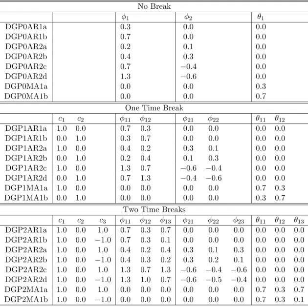
In the case of no breaks, the DGP is given by

DGP0 : yt=φ1yt−1+φ2yt−2+εt−θ1εt−1 : 1≤t≤T,

where the sets of the parameters are summarized in the first panel of Table 1. DGP0AR1a corresponds to the AR(1) case with weak positive serial correlation while yt is moderately

serially correlated for DGP0A1b. DGP0AR2a-b are the AR(2) cases with real valued char-acteristic roots, whereas DGP0AR2c-d have complex roots. We choose these parameters so

that φ1+φ2 = 0.3 (the case of weak serial correlation) or 0.7 (the case of moderate serial

correlation). Similarly, we consider two DGPs for the MA(1) case (DGP0MA1a-b). A process with one time break is generated by

DGP1 :

yt=c1+φ11yt−1+φ21yt−2+εt−θ11εt−1 : 1≤t≤[T /2]

yt=c2+φ12yt−1+φ22yt−2+εt−θ12εt−1 : [T /2] + 1≤t < T,

where the sets of the parameters are given in the second panel of Table 1. For the AR(1) (DGP1AR1a-b) and AR(2) (DGP1AR2a-d) cases, the sum of the AR coefficients changes from 0.7 to 0.3 or 0.3 to 0.7. The MA(1) case (DGP1MA1a-b) has similar structural changes.

The DGP with two time breaks is given by

DGP2 :    yt=c1+φ11yt−1+φ21yt−2+εt−θ11εt−1 : 1≤t≤[T /3] yt=c2+φ12yt−1+φ22yt−2+εt−θ12εt−1 : [T /3] + 1≤t <[2T /3] yt=c3+φ13yt−1+φ23yt−2+εt−θ13εt−1 : [2T /3] + 1≤t < T,

where the sets of the parameters are summarized in the last panel of Table 1. For DGP2AR1a, AR2a, AR2c and MA1a, serial correlation is weakened by the first break but the process returns to the first regime after the second break (the first and third regimes have the same parameters). DGP2AR1b, AR2b, AR2d and MA1b correspond to the case where the level of the process goes down and the process becomes less persistent gradually because of structural changes.

We set T = 120 or 300 while the trimming parameter is set as 0.05 or 0.15. All computations are carried out by using the GAUSS matrix language with 5,000 replications.4 We estimate the AR(py) model including a constant with structural changes and select

the lag lengthpy and the number of breaksmbased on the modified AIC in (12), the modified

Cp criterion in (17) and the two modified BICs in (21) and (22), with a restriction such that the lag lengths are the same in all the regimes. We set ¯py = 4 and ¯m= 5 so that we choose

a model from among 0≤py ≤4 and 0≤m≤5.

To see the effect of our modification, we also estimate py and m by the classical model

selection criteria and Yao’s (1988) modified BIC. In addition, we compare the finite sample performance of the model selection criteria with that of the sequential testing procedure.

4_{We need to efficiently calculate the maximized likelihood for the case of multiple structural changes to}

save computational time. The method is explained in Bai and Perron (1998, 2003) and we made use of the program provided by them.

Since we do not know the true lag length, we first estimate the number of breaks by the testing procedure that is robust to heteroskedasticity and autocorrelation, and then estimate the lag length using the estimated number of breaks. More precisely, following the suggestion by Bai and Perron (2006), we first test for the null of no breaks using the U Dmax test at the 5% significance level allowing different second moments of the regressors as well as the heterogeneity of the variances. Sincepyis unknown, we regressyton a constant in each regime and construct the test statistic using the autocorrelation and heteroskedasticity consistent (HAC) estimate of the variance of the error terms with the prewhitening method. If the null hypothesis is rejected, we continuously use the supF(`+ 1|`) test constructed in the same way as the U Dmax test until it cannot reject the hypothesis. Once the number of breaks is estimated, the lag length is estimated using the Wald test by the general to specific rule. This robust testing procedure is denoted by “Sq(rb)”.

We also consider the hybrid of the modified criteria with the testing procedure; we first estimatepy and m by the modified criteria and using the estimated lag length, estimate the

number of breaks with the testing procedure.5 Note that we do not use the HAC estimates of the variance to construct the test statistics in this case because the lag length is estimated. The hybrid method is denote by “Sq(M IC).” For example, “Sq(M AIC)” signifies that the lag length is selected by the modified AIC while the number of breaks is estimated by the testing procedure.

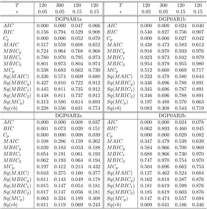
Table 2a reports the frequencies of selecting the true model for the case of no breaks. The entries for the AR(1) and AR(2) cases are the frequencies of ˆpy = 1 and ˆm= 0, respectively. We focus only on the estimation of the number of breaks for the MA(1) case and the entries in this case correspond to the frequencies of ˆm= 0 irrespective of any values of ˆpy, because any

finite order lags are incorrect. From the panels DGP0AR1a-b, we can see that the classical AIC and Cp criterion rarely choose the true model for the AR(1) case while the classical BIC has a better finite sample property when T = 300, although its performance is not necessarily satisfactory when T = 120. This poor finite sample performance of the classical criteria is dramatically improved by our modification; in particular, the modified BICs have

5

We also conducted simulations for the hybrid of the classical model selection criteria, such as AIC and BIC, with the testing procedure, but the performance is poor and we do not report the results.

a high probability of selecting the true model, as expected from Proposition 4. The problem of the classical criteria is that they tend to choose large number of structural changes. For example, in the case of DGP0AR1a with T = 120 and = 0.05 the probabilities for AIC, BIC and Cp when ˆm = 5 and ˆp= 0 are 0.456, 0.403 and 0.475, respectively. This tendency

to over-estimate is well corrected by including the penalty term on the additional breaks. Comparing the modified criteria with the robust testing procedure and the hybrid methods, we find that our modified criteria work better when T = 120. Further, while the hybrid methods perform better than the modified AIC and the modifiedCp criterion in some cases,

they are not as good as the modified BICs in this case. We also note that all the methods perform better for largerT and larger , but the modified criteria are not as sensitive to the value ofas the testing procedure and the hybrid method. In particular, whenT = 120 and

= 0.05, the sequential testing procedure and the hybrid method do not work well.

For the AR(2) case with DGP0AR2a, it is difficult for all the methods to choose the true model. This is because the coefficient associated withyt−2 is so small that shorter lags tend

to be selected. Because the penalty of the modified AIC and the modified Cp criterion is

not as heavy as that of the modified BICs, the former two methods choose the true model with a higher probability. For the other AR(2) case (DGP0AR2b-d) and the MA(1) case (DGP0MA1a-b), the overall performance is similar to the AR(1) case.

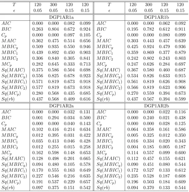
Table 2b reports the result for the case of one time break. As in the case of no breaks, the classical criteria do not perform well because they tend to choose larger breaks; this tendency to over-estimate is fixed by our modification. In this case, while the hybrid method with the modified BICs tends to choose the true model more frequently than the modified BICs for the AR(1) and AR(2) cases, the relation is reversed for the MA(1) case. However, the performance of both the methods is not satisfactory for DGP1AR2a-b.

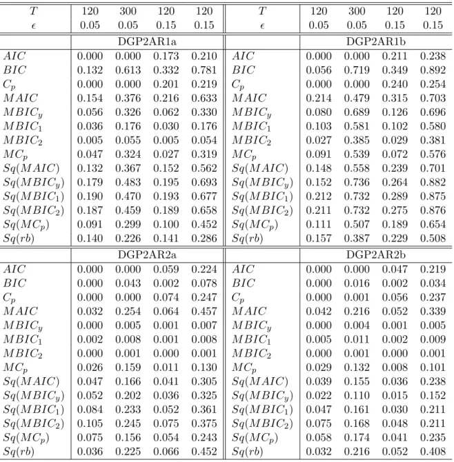
The result for the case of two time breaks is summarized in Table 2c. As a whole, it seems difficult to choose the true model for the AR(1) and AR(2) cases, especially, whenT = 120. The modified AIC works best among the modified criteria but its performance is dominated by the hybrid method in many cases. On the other hand, the modified BICs work better than the hybrid method for the MA(1) case, although both perform quite well in this case.

To summarize our simulation results, we can say that the modified BICs perform relatively well when m0 ≤ 1 and = 0.05, while the hybrid method with the modified BICs, that is, the sequential testing procedure with the lag order selected by the modified BICs, may be recommended if one is confident that the distance between the two consecutive break fractions is not so close, such as= 0.15, or if it is believed that the model has more than one break with a high probability.

5. Conclusion

This paper developed the model selection criteria to select the regressors and the number of structural changes in multivariate regression models, including a VAR model as a special case. We derived the modified AIC, the modifiedCp criterion and the modified BICs. The penalty terms of these criteria are determined not in ad hoc ways but based on the risk functions given for the criteria. We showed that the modified BICs can consistently estimate the number of structural changes and the regressors while the modified AIC and the modifiedCp criterion

tend to choose a larger model with a positive probability. The consistency of the modified BICs is a plausible theoretical property and by reflecting this nice nature, the modified BICs perform well in finite samples. Because it is important to consistently estimate the number of breaks and given the simulation results, the modified BICs and the hybrid method are recommended to be implemented for practical analyses.

Appendix

Since all the model selection criteria are derived when m=m0 and p =p0, we omit the superscript 0 for notational convenience.

Proof of Lemma 1: In this proof we omit a subscript j for notational convenience. For example, B1j(v) is abbreviated as B1(v). As explained in Appendix B of Bai (1997a),

maxv≤0B1(v) and maxv>0B2(v) are distributed as exponential distributions with

param-etersγ1/ω1 and γ2/ω2, respectively, and hence

P max v B I_{(v)≤b = P} max max v≤0 B1(v), maxv>0 B2(v) ≤b = P max v≤0 B1(v)≤b P max v>0 B2(v)≤b

= 1−e−(γ1/ω1)b _1−e−(γ2/ω2)b

,

where the second equality holds becauseB1(v) and B2(v) are independent. Then, the

prob-ability density function of maxvBI(v) is given by

f(b) = (γ1/ω1)e−(γ1/ω1)b+ (γ2/ω2)e−(γ2/ω2)b− {(γ1/ω1) + (γ2/ω2)}e−{(γ1/ω1)+(γ2/ω2)}b.

Carrying out the integration R

b>0bf(b)dband letting r1 =ω1/γ1 and r2 =ω2/γ2, we obtain

(5).

Next, let ˆv = argmax_vBI(v). By change of variable with s = (γ₁2/ω1)v as in Qu and

Perron (2007) we can see that ˆ v= ω1 γ₁2 argmaxs ˜ BI(s), where B˜I(s) = W1(|s|)−|₂s| : s≤0 √ rωW2(s)−s₂rγ : s >0,

whererω =ω2/ω1andrγ =γ2/γ1. Then, it is sufficient to calculateE[argmaxsB˜I(s)1(s≤0)]

andE[argmax_sB˜I(s)1(s >0)] in order to obtain (6) and (7).

Following Appendix B of Bai (1997a) it can be shown that the probability density function (pdf) of ˆs= argmax_sB˜I(s) is given by g(s) =          −1 2Φ −1 2 p |s|+rγ rω + 1 2 e(1/2){(rγ/rω)+(rγ/rω)2}|s|_Φ −rγ rω + 1 2 _p |s| : s≤0 −(rγ/ √ rω)2 2 Φ −(rγ/ √ rω) 2 √ s + rγ+(rγ/ √ rω)2 2 e(1/2)(rγ+rω)s_Φ −√rω+(rγ/ √ rω) 2 √ s : s >0 ,

which is obtained based on the result on an additive process by Bhattacharya and Brockwell (1976),6 where Φ(·) denotes a cumulative distribution function of a standard normal random variable. By carrying out the integration we obtain

Z 0 −∞ sg(s)ds=−2rγ(rγ+ 2rω) (rγ+rω)2 =− 2r1(r1+ 2r2) (r1+r2)2 , Z ∞ 0 sg(s)ds= 2r 2 ω(rω+ 2rγ) r2 γ(rγ+rω)2 = 2 rγ r₂2(2r1+r2) r1(r1+r2)2 ,

where the second equalities of the above two integrals are obtained by usingrω= (r2/r1)rγ.

Noting that E aI_j argmax s ˜ BI(s) =a2 Z ∞ 0 sg(s)ds−a1 Z 0 −∞ sg(s)ds,

6_{This result is obtained by replacingφandξ in Bai (1997a) withr}

ω andrγ, respectively. Note that there are typos in equation (B.1) and the definition ofg(x) in Bai (1997a). The first term on the right hand side of

E aI_jargmax s ˜ BI(s) =a2 Z ∞ 0 sg(s)ds+a1 Z 0 −∞ sg(s)ds,

(6) and (7) are established.

Proof of Proposition 1: In this proof we restrict our analysis on the set given by{Tj|Tj =

T0

j +cv

−2

T , −M ≤ c ≤ M} for some large M (j = 1,· · · , m) because ˆTj −Tj = Op(v

−2

T )

as shown by Qu and Perron (2007). We first evaluatebm,px,1. SinceEy[`m,px(T

0_{, θ}0_{|y, x)] =}

−(nT /2) log(2π)−(1/2)Pm+1

j=1 ∆Tj0log|Σ0j| −(nT /2), we can see that

`m,px( ˆT,θˆ|y, x)−E `m,px(T 0_{, θ}0_{|y, x)} =R11+R12, (25) where R11=− m+1 X j=1 ∆ ˆTj 2 log|Σˆj| − ∆T0 j 2 log|Σ 0 j| ! , R12=− m+1 X j=1 ∆ ˆTj 2 log|Σˆj| −log|Σ0j| − m+1 X j=1 ∆ ˆTj−∆Tj0 2 log|Σ 0 j|.

By expanding log|Σˆj|around log|Σ0j|,R11 is expressed as

R11 = − m+1 X j=1 ∆ ˆTj 2 tr n Σ0_j−1 ˆ Σj−Σ0j o −1 2tr n Σ0_j−1 ˆ Σj−Σ0j Σ0_j−1 ˆ Σj−Σ0j o +op(1) = − m+1 X j=1 ∆ ˆTj 2 h tr n Σ0_j−1 ˆ Σj −Σ˜j o + tr n Σ0_j−1 ˜ Σj−Σ0j o −1 2tr n Σ0_j−1Σˆj −Σ0j Σ0_j−1Σˆj−Σ0j o +op(1), (26) where ˜Σj =P T0 j t=T0 j−1+1 ˜ εtε˜0t/∆ ˆTj with ˜εt=yt−(xt0 ⊗In) ˆφj forTj0−1+ 1≤t≤Tj0.

For ˆTj < Tj0, the first term in the square brackets on the right hand side of (26) becomes

− m+1 X j=1 ∆ ˆTj 2 tr n Σ0_j−1 ˆ Σj−Σ˜j o = −1 2 m X j=1 T0 j X t= ˆTj+1 n εt−(x0t⊗In)( ˆφj+1−φ0j) o0 Σ0_j+1−1nεt−(xt0 ⊗In)( ˆφj+1−φ0j) o −nεt−(x0t⊗In)( ˆφj−φ0j) o0 Σ0_j−1nεt−(xt0 ⊗In)( ˆφj−φ0j) o = −1 2 m X j=1 T0 j X t= ˆTj+1 trΣ0_j−₊₁1εtε0t −trΣ0_j−1εtε0t

−2( ˆφj+1−φ0j)0 T0 j X t= ˆTj+1 xt⊗Σ0_j+1−1 εt+ ( ˆφj+1−φ0j)0 T0 j X t= ˆTj+1 xtx0_t⊗Σ0_j−₊₁1 ( ˆφj+1−φ0j) +op(1). Since ˆφj+1−φ0j = (φ0j+1−φ0j) + ( ˆφj+1−φ0j+1) =vTδj +Op(1/ √ T) and Σ0_j−1 = Σ0_j−₊₁1+ Σ_j0−₊₁1(Σ0_j+1−Σ0_j)Σ0_j+1−1+ Σ0_j+1−1(Σ0_j+1−Σ0_j)Σ_j0−1(Σ0_j+1−Σ0_j)Σ0_j+1−1 = Σ0_j−₊₁1+vTΣ 0−1/2 j+1 A2jΣ 0−1/2 j+1 +v 2 TΣ 0−1/2 j+1 A 2 2jΣ 0−1/2 j+1 +O(v 3 T),

we can see that, for ˆTj < T_j0,

− m+1 X j=1 ∆ ˆTj 2 tr n Σ0_j−1Σˆj −Σ˜j o = 1 2 m X j=1 tr  v_TA_1j Tj0 X t= ˆTj+1 ηtηt0  −v_T2(T_j0−Tˆ_j)tr A2_1j +2vTδ_j0 T0 j X t= ˆTj+1 xt⊗Σ0_j−1 εt−v_T2δ_j0 T0 j X t= ˆTj+1 xtx0_t⊗Σ0_j−1 δj+op(1). (27)

Similarly, the second and third terms in the square brackets on the right hand side of (26) are expressed as − m+1 X j=1 ∆ ˆTj 2 tr n Σ0_j−1( ˜Σj−Σ0j) o = −1 2 m+1 X j=1 T0 j X t=T0 j−1+1 n εt−(x0_t⊗In)( ˆφj −φ0_j) o0 Σ0_j−1 n εt−(x0_t⊗In)( ˆφj−φ0_j) o +nT 2 = 1 2 m+1 X j=1 ( ˆφj−φ0j) Tj0 X t=T0 j−1+1 xtx0t⊗Σ0j−1 ( ˆφj −φ0j)− 1 2 m+1 X j=1 tr      Tj0 X t=T0 j−1+1 ηtη0t−In      +op(1). (28) m+1 X j=1 ∆ ˆTj 4 tr n Σ0_j−1Σˆj−Σ0j Σ0_j−1Σˆj −Σ0j o = m+1 X j=1 1 4∆T_j0tr         T0 j X t=T0 j−1+1 (ηtη0t−In)    2     +op(1). (29) On the other hand, R12 becomes, for ˆTj < Tj0,

R12 = 1 2 m X j=1 (T_j0−Tjˆ) log|Σ0_j| −log|Σ0_j+1|

= 1 2 m X j=1 T0 j X t= ˆTj+1 tr (−vTA1j) + v2_T(T_j0−Tjˆ) 2 tr A 2 1j +op(1), (30)

where the last equality is obtained by expanding log|Σ0_j+1|around log|Σ0_j|.

Then, by combining (27)–(30), we have, for ˆTj < T_j0,

R11+R12+ 1 2 m+1 X j=1 tr      T_j0 X t=T0 j−1+1 ηtη0t−In      = 1 2 m+1 X j=1 ( ˆφj−φ0_j) T0 j X t=T_j0−1+1 xtx0_t⊗Σ0_j−1 ( ˆφj −φ0_j) + m+1 X j=1 1 4∆T0 j tr         T0 j X t=T_j0−1+1 (ηtη0_t−In)    2     + m X j=1 tr    vT 2 A1j T0 j X t= ˆTj+1 ηtη_t0−In    −v 2 T 4 (T 0 j −Tjˆ)tr A21j +vTδj0 T0 j X t= ˆTj+1 xt⊗Σ0j−1 εt− v2_T 2 δ 0 j T0 j X t= ˆTj+1 xtx0t⊗Σ0j−1 δj+op(1) d −→ 1 2 m+1 X j=1 χ2_p φj + m+1 X j=1 κ4j 4 + m X j=1 max v B I j(v), (31) whereχ2

p_φj (j = 1,· · ·, m+ 1) are independent chi-square distributions with pφj degrees of

freedom. Since the same convergence holds for ˆTj > Tj0 and the expectation of the left hand

side of (31) equalsbm,px,1, we can see using Lemma 1 that, up to theO(1) terms,

bm,px,1 = pall_φ 2 + m+1 X j=1 κ4j 4 + m X j=1 r₁2_j+r1jr2j+r22j r1j+r2j .

We next evaluatebm,px,3 because bm,px,2= 0 is obvious. Since

Ey∗[`m,p x(T 0_,θˆ|y∗ , x∗)] = −nT 2 log(2π)− m+1 X j=1 ∆T0 j 2 log|Σˆj| − 1 2 m+1 X j=1 T0 j X t=T0 j−1+1 tr ˆ Σ−_j1Σ0_j −1 2 m+1 X j=1 ∆T_j0( ˆφj−φ0_j)0Ey∗[x∗_tx∗0_t ]⊗Σˆ−1 j ( ˆφj−φ0_j),

we can see that Ey∗[`<sub>m,p</sub> x(T 0<sub>, θ</sub>0<sub>|y</sub>∗<sub>, x</sub>∗<sub>)]−E</sub> y∗[`_m,p x(T 0_,θˆ|y∗_{, x}∗_)] = m+1 X j=1 ∆T_j0 2 log|Σˆj| −log|Σ0j| −nT 2 + 1 2 m+1 X j=1 T_j0 X t=T0 j−1+1 trΣˆ−_j1Σ0_j +1 2 m+1 X j=1 ∆T_j0( ˆφj −φ0_j)0 Ey∗[x∗_tx∗0_t ]⊗Σˆ−1 j ( ˆφj−φ0_j) = m+1 X j=1 ∆T_j0 4 tr n Σ0_j−1( ˆΣj −Σ0j)Σ0j−1( ˆΣj−Σ0j) o +1 2 m+1 X j=1 ∆T_j0( ˆφj −φ0_j)0 Ey∗[x∗ tx ∗0 t ]⊗Σˆ −1 j ( ˆφj−φ0_j) +op(1) d −→ m+1 X j=1 κ4j 4 + 1 2 m+1 X j=1 χ2_p φj, (32)

where the second equality is obtained by expanding log|Σˆj|around log|Σ0j|and by using the

relation tr ˆ Σ−_j1Σ0_j =n−tr n Σ0_j−1( ˆΣj −Σ0j) o + tr n Σ0_j−1( ˆΣj−Σ0j) ˆΣ −1 j ( ˆΣj−Σ 0 j) o ,

which holds because ˆ Σ_j−1= Σ0_j−1−Σ_j0−1( ˆΣj−Σ0j)Σ0 −1 j + Σ 0−1 j ( ˆΣj−Σ 0 j) ˆΣ −1 j ( ˆΣj −Σ 0 j)Σ0 −1 j .

From (32), we have, up to theO(1) terms,

bm,px,3=Ey h Ey∗[`<sub>m,p</sub> x(T 0<sub>, θ</sub>0<sub>|y</sub>∗<sub>, x</sub>∗<sub>)]−E</sub> y∗[`_m,p x(T 0_,θˆ|y∗_{, x}∗_)]i₌ m+1 X j=1 κ4j 4 + pall_φ 2 . Forbm,px,4, we write Ey∗[`<sub>m,p</sub> x(T 0<sub>,θˆ|y</sub>∗<sub>, x</sub>∗<sub>)]−E</sub> y∗[`_m,p x( ˆT,θˆ|y ∗_{, x}∗_{)] =R} 41+R42+R43, where R41= m+1 X j=1 ∆ ˆTj−∆Tj0 2 log| ˆ Σj|, R42= 1 2 m+1 X j=1 ˆ Tj X t= ˆTj−1+1 n y∗_t −(x∗0_t ⊗In) ˆφj o0 ˆ Σ−_j1ny_t∗−(x∗0_t ⊗In) ˆφj o ,

R43=− 1 2 m+1 X j=1 T0 j X t=T0 j−1+1 n y_t∗−(x∗0_t ⊗In) ˆφj o0 ˆ Σ−_j1 n y_t∗−(x∗0_t ⊗In) ˆφj o .

Similarly to the evaluation of R12, by the Taylor expansion of log|Σˆj+1|, R41 can be

expressed as, for ˆTj < Tj0,

R41 = m X j=1 ˆ Tj−T_j0 2 log|Σˆj| −log|Σˆj+1| = 1 2 m X j=1 (T_j0−Tjˆ) h tr n ˆ Σ−_j1 ˆ Σj+1−Σˆj o −1 2tr n ˆ Σ−_j1Σˆj+1−Σˆj ˆ Σ−_j1Σˆj+1−Σˆj o +op(1). (33)

On the other hand, R42+R43 becomes, for ˆTj < Tj0,

R42+R43 = Ey∗   1 2 m X j=1 T0 j X t= ˆTj+1 n ε∗_t −(x∗0_t ⊗In)( ˆφj+1−φ0j) o0 ˆ Σ−_j+11 nε∗_t −(x_t∗0⊗In)( ˆφj+1−φ0j) o −nε∗_t −(x∗0_t ⊗In)( ˆφj−φ0j) o0 ˆ Σ−_j1nε∗_t −(x_t∗0⊗In)( ˆφj−φ0j) o = 1 2 m X j=1 (T_j0−Tˆj)vT2δj0 E[x∗_tx∗0_t]⊗Σˆ_j−₊₁1 δj −(Tj0−Tˆj)tr n ˆ Σ−_j1Σˆj+1−Σˆj ˆ Σ−_j1Σ0_jo +(T_j0−Tˆj)tr n ˆ Σ−_j1Σˆj+1−Σˆj ˆ Σ−_j+11 Σˆj+1−Σˆj ˆ ΣjΣ0j o +op(1). (34)

Thus, by combining (33) and (34), we have, for ˆTj < Tj0,

Ey∗[`<sub>m,p</sub> x(T 0<sub>, θ</sub>0<sub>|y</sub>∗<sub>)]−E</sub> y∗[`_m,p x(T 0_,θˆ|y∗_)] = m X j=1 v_T2(T_j0−Tˆj) 1 2δ 0 j E[x∗_tx∗0_t ]⊗Σˆ−_j1δj+ 1 4tr A 2 1j +op(1) d −→ m X j=1 γI_j 2 argmax v B_jI(v) ,

whereγ_jI =γ1j when v≤0 and γjI =γ2j whenv >0. Since the same convergence holds for

ˆ Tj > T_j0, we have, by Lemma 1, bm,px,4 =Ey h Ey∗[`m,p x(T 0<sub>, θ</sub>0<sub>|y</sub>∗<sub>)]−Ey</sub> ∗[`m,p x(T 0_,θˆ|y∗_)]i₌ m X j=1 r₁2_j +r1jr2j+r22j r1j+r2j (35)

up to theO(1) terms.

Proof of Proposition 2: E[Jm,px,1] = −nT is obvious. For Jm,px,2 we expand it as, for

ˆ Tj < T_j0, Jm,px,2 = 2 m+1 X j=1 T0 j X t=T0 j−1+1 (ˆµt−µt˜ ) + (˜µt−µ0_t) 0Σ0_j−1εt = 2 m X j=1 T_j0 X t= ˆTj+1 n (x0_t⊗In)( ˆφj+1−φˆj) o0 Σ0_j−1εt +2 m+1 X j=1 T0 j X t=T0 j−1+1 n (x0_t⊗In)( ˆφj−φ0_j) o0 Σ0_j−1εt = 2 m X j=1 vTδ_j0 T0 j X t= ˆTj+1 xt⊗Σ0_j−1 εt−vTδ_j0 T0 j X t= ˆTj+1 xtx0_t⊗Σ0_j−1 δj +vTδ0j T0 j X t= ˆTj+1 xtx0t⊗Σ0j−1 δj +2 m+1 X j=1 ( ˆφj−φ0_j)0 T0 j X t=T_j0−1+1 xtx0_t⊗Σ0_j−1 ( ˆφj−φ0_j) +op(1) d −→ m X j=1 2 max v B I j(v) +γjI argmax v B_jI(v) + 2 m+1 X j=1 χ2_p φj,

where, under the assumption of Σj+1−Σj = vT2Ψj, γjI = γ1j = δj0Q1jδj when v ≤ 0 and γ_jI =γ2j =δj0Q2jδj when v >0,BIj(v) is defined as (4) withω1j =γ1j =δj0Q1jδj and ω2j = γ2j = δj0Q2jδj because only the changes in the coefficients affect the limiting distributions

of the break points in this case. Note that the same convergence holds for ˆTj > T_j0. From Lemma 1 we can see that

Eh2 max v B I j(v) i =E γ_jI argmax v BI_j(v) = 3 in this case. Hence, we obtainE[Jm,px,2] = 6m+ 2p

all