(IJSBAR)
ISSN 2307-4531
(Print & Online)
http://gssrr.org/index.php?journal=JournalOfBasicAndApplied
---
143
Applying Bootstrap Robust Regression Method on Data
with Outliers
Ahmed M. Mami
a*, Abobaker M. Jaber
b, Osama S. Almabrouk
ca,b,cDepartment of Statistics, Faculty of Science, University of Benghazi, Benghazi, +128, Libya a Email: [email protected] b Email: [email protected] cEmail: [email protected] Abstract
Identification and assessment of outliers have a key role in Ordinary Least Squares (OLS) regression analysis. This paper presents a robust two-stage procedure to identify outlying observations in regression analysis. The exploratory stage identifies leverage points and vertical outliers through a robust distance estimator based on Minimum Covariance Determinant (MCD). After deletion of these points, the confirmatory stage carries out an OLS analysis on the remaining subset of data and investigates the effect of adding back in the previously deleted observations. Cut-off points pertinent to different diagnostics are generated by bootstrapping and the cases are definitely labeled as good-leverage, bad leverage, vertical outliers and typical cases. This procedure is applied to four examples taken from the literature and it is effective in rightly pinpointing outlying observations, even in the presence of substantial masking. This procedure is able to identify and correctly classify vertical outliers, good and bad leverage points, through the use of jackknife-after-bootstrap robust cut-off points. Moreover its two stage structure makes it interactive and this enables the user to reach a deeper understanding of the dataset main features than resorting to an automatic procedure.
Keywords: regression analysis; outliers; robust regression; bootstrap.
--- * Corresponding author.
144
1. Introduction
One of the most famous methods of data analysis that aimed to discover how one or more variables affect other variables is called “regression”. Outliers are major problem in regression analysis and consider being a serious threat to standard least squares analysis. The definition of the term "outlier" is any observation which deviates from the pattern set by the majority of the data. Also, it may define as any observation that is far from the bulk of the data. Therefore, the usage of robust regression is needed in order to reduce the effect of outliers. Despite its mathematical beauty and computational simplicity, the ordinary least squares (OLS) estimator dramatically lacks this preferred robustness. For instance, a single outlier can have a large arbitrary effect on the estimate. In this paper, the main goal is to find a better robust regression estimator to reduce the influence of outliers. Thus, we propose using four different robust regression estimators to deal with the problem of Outliers in the data with employing the bootstrap techniques. The main purpose of using the bootstrap is to give rise to the robust estimators. These estimators are namely as: the Least Median Square (LMS), the M-estimator (MM), Bootstrap M-estimator (BMM), and the Fast Bootstrap M-estimator (FBM). In order to achieve our goal, we perform 324 simulation studies for data contains different distributions of marginal errors, different sample sizes and a variety of percentages of outliers, and three different patterns of outliers directions through utilizing the four proposed robust regression estimators. Applications on real data also have been considered especially when there exist a mixed variables as well as the presence of Outliers observations. Several interesting features have been noted from this study. One of the most striking point is that the bootstrap robust regression estimators (BMM estimator and FBM estimator) are much efficient than the LMS, MM, and OLS estimators when the outliers are present, regardless of the data sample size, the errors' marginal distribution, and the direction of outliers. Therefore, employing the bootstrap technique within the robust regression context can provide a very beneficiary result.
1.1 Outliers
The definition of the term "outlier" is any observation which deviates from the pattern set by the majority of the data. Also, it may define as any observation that is far from the bulk of the data. Typing and recording data may produce outliers, and any data set can have a large proportion of outlier's acts differently for each variable. Recording errors can often be corrected and omitted variables can also be included. However, there is no simple explanation for a group of data that differs from the majority of the data [24]. Outliers will cause a weak linear relationship to appear as a strong linear relationship, or may have the opposite effect by masking a strong linear relationship. Moreover, Outliers tend to have a stronger effect when the sample size n is small than when the sample size n is large. Therefore, Outliers may have a dramatic impact on results of regression analyses, potentially having major influence on effects sizes and regression coefficients [21].
1.2 Detecting of Outliers
Outlier detection methods must involve the use of statistics that are obtained for each case (observation). Three categories of detection measures are generally used, namely
145
Leverage: Extremity of each observation on the Explanatory Variables. Discrepancy: Extremity of each observation on the Response variable. Influence: Influence of each observation on regression results [1].
1.2.1 Leverage Measures
The Leverage Measures assess the extremity (i.e the typicality) of each observation on the Explanatory variables. Extreme observations have the potential to have great influence on results of regression analyses. When there is only one explanatory variable, the usual measure of leverage is given by
̅̅̅̅
∑ (1.1)
Where
h
ii is the ith element on the main diagonal of the hat matrix. The hat matrix can be defined as
Observations near the mean of X produce low values of
h
ii, whereas observations further from the mean produce larger values. This measure of leverage can be extended to the case ofp
explanatory variables. In general, Observations near the joint mean of the distribution of the Explanatory variables yield low values of Leverageh
ii, and cases further away from the joint mean yield larger values. Once we obtain values, one for each of the n observations, we need to examine them to identify extreme values. The Common Cut-off values areh
ii>2(p+1)/n orh
ii>3(p+1)/n.1.2.2 Discrepancy Measures
The Discrepancy Measures assess extremity on the Response variable of the regression model. A simple measure of extremity would be the regression residual for each case:
̂
Recall that, any extreme observation
i
will influence the regression line in such a way as to make the corresponding residual smaller for that observation. An improved measure of discrepancy for casei
would be the value of the residual that would be obtained if that case were not included in the regression model. This value is calculated bŷ
Where
ˆ
i(i)is the predicted value of Y that would be obtained for casei
using a regression equation derivedii
h
146
from the sample excluding case
i
. Observations exhibiting a large value of are cases that are deviant in terms of their residuals when the regression equation is derived based on the rest of the sample. To put these values on a standardized scale we define
These values are called Studentized residuals [20]. We then wish to identify extreme values by using the cutoff values. Since these residuals approximately follow a t-distribution, common cutoffs are ±2 in small to moderate samples, and ±3 or ±4 in large samples. By this process we can identify observations that are highly discrepant on the Response variables in the regression model estimation process.
1.3 Influential Observations Measures
There are three kinds of influence observations measures, namely:
Influence on a single Fitted Value
Well-known influence measure assesses the change in the predicted Y value as a function of whether an observation,
i
, is included in the sample or not. For each case i we obtain a measure called DFFITSi, and is calculated bŷ ̂
√
If
then the case is influential case [1].
Influence on All Fitted Values
Another commonly used index called Cook’s distance, and is calculated by
If the value i
d
n
p
i
DFFITS
2
(
1
)
)
)
1
(
(
)
1
(
2 2 2 ii ii i ih
h
p
s
e
D
p
1
)
n
(
4
D
i
147
then the case is influential case. This process helps us to identify observations that have a relatively large global influence on the results of the regression model estimation process [6].
Influence on Specific Regression Coefficients
In some situations, we may be interested in whether those particular coefficients might be highly influenced by outliers. Such influences can be assessed using an index called DFBETA. We can calculate a DFBETA value for each case,
i
:
√
Where Coefficient
b
k obtained from the full sample, andb
k(i) is the regression coefficient obtained when casei
is excluded from the sample. This value represents the influence of observationi
on the regression coefficient
j. Once we obtain one of these measures for each case we again seek to identify extreme values using cutoffs are ±1 for small to moderate n, and larger values such as
2
/
n
when n is large [20].2. Robust Regression Models
2.1 Definition of Robustness
Robustness is an important issue for all statistical analyses. The term robustness comes to signify the insensitivity to small deviations from the assumption [18]. Diagnostics and Robust regression have the same objectives, but in the opposite order. When using diagnostic devices, we first tries to delete the outliers and then to fit the good data by the Ordinary Least Squares (OLS). On the other side, in the Robust analysis, we first want to fit a regression to the majority of the data and then try to discover the outliers as those points which possess large residuals from that robust solution [26]. In order to describe the robustness of an estimator, Hample (1971) had proposed two different and complementary ways, called Global Robustness, and Local Robustness [18].
2.2 Global Robustness
Hample (1971) had introduced the concept of breakdown point as a measure of comparison of performance among different robust techniques. The breakdown of an estimator is defined as the smallest proportion of the data that can have an arbitrary large effect on its value. Therefore, high breakdown is favorable and the largest value of it is 50%. The sample median is less sensitive to observation values and unless more than half of the observations are bad it does not totally break down, hence it has breakdown 50% [25].
2.2.1 Least Median of Squares (LMS) Estimator
148
developed by Rousseeuw (1984) is defined as follows:Let the vector minimizing the following objective:
Minimize median (2.1)
Where the residuals equals
y
i
X
i1
1
X
ip
p
. Obviously, the breakdown point of this estimator is 50%, which means that it remains bounded when up to half of the data points
i,
y
i
are replaced by arbitrary values. Comparing with the breakdown point of the OLS estimators which equals to 0% .There are several interesting properties of LMS estimator:
1. There always exists a unique solution for the LMS estimator.
2. The LMS estimator is regression equivariant, scale equivariant and affine equivariant.
3. If the number of the explanatory variables (p) > 1 and the the number of observations (n), then the breakdown point of the LMS estimator is:
The major disadvantage of the LMS estimator is the lack of efficiency when errors would really be normally
distributed. The convergence rate of the LMS estimator is only 3
1
n
as the convergence rate of the asymptotically normal estimators is 21
n
. The LMS estimator is not asymptotically normal [16].2.3 Local Robustness
The basic idea of this concept is to measure the effect of a single outlier on the bias and variance respectively. Only the influence function will be considered here [27]. The influence function in regression analyses can be defined as follows:
Let
(
x
1,
y
1),...,
(
x
n,
y
n)
represents a bivariate data, which can be modelled by the following linear regression modeli i
i
x
e
y
(2.3)It is appropriate to include 1 as the first component of
x
i so thatx
i
(
1
,
x
i1,...,
x
ip)
andip p i i
x
x
x
0
1 1
...
.
P
T
ˆ
1,...
.,
ˆ
T
r
i2
ir
)
2
.
2
(
2
/
)
2
]
2
/
([
*
p
n
149
Let the statistic
(
x
1,
y
1,...
.,
x
n,
y
n)
be an estimate of
calculated from the sample .In order to define the influence function of estimate, we regard the explanatory variables, and the response variable, as being random. Let
n denote the empirical probability distribution that assigns probability to each data point ()
,
ii
y
x
, and express the statistic
(
x
1,
y
1,...
.,
x
n,
y
n)
as a function of
n. The OLS estimate of
can be written as
(
n)
such that)
(
E
)
(
E
)
P
(
T
n
p
1 P
(2.4)Where
x
,
y
are random vectors with distribution
. Thus, the influence functionIF
(
,
)
of the estimate)
,
.,
,...
,
(
x
1y
1x
ny
n
can be defined as the vector of derivatives of
((
1
)
n
(,) with respect to
at
0
. Therefore, theIF
(
,
)
will give the rate of change of the estimate when a small proportion of any additional data with values (
,
)
is included in the sample. For the OLS estimate,)
,
(
IF
=n
(
x
x
)
1w
(
ˆ
olsew
)
(2.5)For more comprehensive details see (David Birkes. Yadolah Dodge). In the literature, there are two robust methods known as influence functions (The Least Absolute Deviation and The estimation). The M-estimation method is one of interest in this work.
2.3.1 The M-Estimation Method
The most famous method of robust regression is the M-estimation. Huber [17] was the first to introduced M -estimator. The M-estimators are statistically more efficient (for regression models with Gaussian error) then
OLS estimators, while at the same time they still robust with respect to outlying observations
i [13]. Let us consider the fitted linear regression model in the matrix notation, for the ith case of n observations:)
6
.
2
(
ˆ
ˆ
1X
Y
nThe basic idea of the M-estimator is to minimize the following objective function:
)
7
.
2
(
)
ˆ
(
)
(
1 1
n i i i n i ie
Where the function
gives the contribution of each residual to the objective function. A reasonable
should have the following properties:150
(
e
)
0
(
e
)
0
(
e
)
(
e
)
(
e
i)
(
e
i)
for
e
i
e
i .For example, for the least squares estimation,
(
)
(
)
2
i i
e
e
.Let
be the derivative of
. Differentiating the objective function with respect to the coefficients,
ˆ
and setting the partial derivatives to 0, produces a system ofk
1
estimating equations for the coefficients:
n i 1)
ˆ
ˆ
(
Define the weight function as
(
e
)
(
e
i)
(
e
)
/
e
, and let
i
(
e
i)
. Then the estimating equations be rewritten as:)
8
.
2
(
0
)
(
1
i i n i i
Solving such estimating equations is simply a weighted least-squares problem, thus by minimizing
n i i ie
1 2 2
The weights, however, depend upon the residuals, the residuals depend upon the estimated coefficients, and the estimated coefficients depend upon the weights.
The Iteratively Reweighed Least Squares (IRLS) is required in order to obtain the solution, which is performed in the following algorithm:
1. Select initial estimates
(0), such as the OLS estimates.2. At each iteration
t
, calculate residualse
i(t1) and associated weights
i(t1)
i
e
i(t1) from the previous iteration.3. Solve for new weighted least squares estimates
(
2
.
9
)
ˆ
t
(t1)
1
(t1)
W
W
151
Where
is the model matrix, with
i as its ith row, andW
(t1)
diag
{
i(t1)}
is the current weight matrix.4. Step 2. and Step3. are repeated until the estimated coefficients converge. The asymptotic covariance matrix of
ˆ
is:
(
)
)(
)
(
2
.
10
)
/
)
(
(
)
ˆ
(
2
2
Using
2)
(
e
i to estimate
(
2)
, and
2/
)
(
e
in
to estimate
(
)
2 produces the estimated asymptotic covariance matrix,
ˆ
(
ˆ
)
[13], and [16].Keep in mind that the IRLS solution is not equivariant with respect to scale. Therefore, the residuals should be standardized by means of some estimate of the standard deviation
so that:)
11
.
2
(
0
)
ˆ
/
(
1
n i i ir
Where
ˆ
is the Median Absolute Deviation (MAD) scale estimator, and can be obtained as)
12
.
2
(
)
)
(
(
*
ˆ
1ri
med
r
C
i n i
Where
C
=1.4826 if the error terms distributed as normal.In conclusion, the MM estimator is the most used in the robust estimation context. The letter M indicates that the M estimation is an estimation of the maximum likelihood type. A more detailed description is available in, e.g., [28,27,3,11,13]
2.4 The Principle of Bootstrap in Regression
The Bootstrap technique was introduced by [9]. Simply, Bootstrapping is a general approach to statistical inference based on replacement of the true sampling distribution for a statistic by resampling from the original observed data of size n. Therefore, Bootstrap technique assumes only finite values of some moments, but hardly any restricting assumptions about the underlying probability distribution. The central element of bootstrap is a bootstrap sample For more comprehensive details see.[5,7,14,10,29]. In the bootstrap regression procedure, the Ordinary Least Squares (OLS) method is often used to estimate the parameters of regression models. It is, however, extremely sensitive to outliers and non-normality of errors. The robust bootstrapping method replaces the classical bootstrap mean and standard deviation with robust estimates, using robust regression estimates with a high breakdown point. In this thesis, MM regression with initial Least Median of Squares LMS
152
estimates has been used. The bootstrap is not used for regression parameters estimation, being a tool for the acquisition of confidential intervals and bias regression parameters estimation.
2.5 The Proposed Estimators of the Study
The following regression methods have been considered in this work:
Ordinary Least Squares regression (OLS), Least Median of Squares regression (LMS), MM-regression (MM),
Bootstrap regression based on the MM method (BMM),
Fast Bootstrap regresion based on robust MM-regression (FBM)
3. The Simulation Study
The main goal of this section is to compare the performance of the five proposed estimators that used to deal with the problem of outliers. In the simulation study, all computations and graphics were carried out using the software package R, which based on the statistical language S (Statistical Science, Inc. 2005).
3.1 The Illustration of the Experiment
The simulated data, in this study, represented many situations that we often encounter when using the regression analysis. Since there are various situations of outliers on the regression model, we decided to consider three different arrangements depending on the number of explanatory variables (the simple case: p=1, and the multiple cases: p=2, and p=5). Each set was generated in three different settings, as:
Setting 1: Outliers are located in the y-direction,
Setting 2: Outliers are located in the x-direction and
Setting 3: Outliers are located in the xy-direction
Three different sample sizes are considered n = 30, 50, and 100 with the regression model which has the form Y= . In each of three different setting mentioned above, we shall obtained, (1 )% of them were outliers. Experimenting with different random sample sizes n when p = 1 for a simple linear regression and when p = 2, and 5 for multiple linear regression, the simulated data are obtained. Also, three different percentages of outliers 10%, 20%, 50% were considered. Finally, four different distributions of marginal errors were also considered, namely: the normal distribution, the exponential distribution, the uniform distribution and , the heavy-tailed t distribution.
153
Figure 3.1:The Box plots exhibit how various proportions of outliers affect the mean (standard deviations) of the MSE values for the five proposed estimators (OLS, LMS, MM, BMM, and FBM) with different choices of
sample sizes assuming the proposed marginal errors belongs to Normal distribution with p=1 and outliers are located in XY-direction.
Figure 3.2:The Box plots exhibit how various proportions of outliers affect the mean (standard deviations) of the MSE values for the five proposed estimators (OLS, LMS, MM, BMM, and FBM) with different choices of
sample sizes assuming the proposed marginal errors belongs to t distribution with p=1 and outliers are located in XY-direction.
154
Figure 3.3:The Box plots exhibit how various proportions of outliers affect the mean (standard deviations) of the MSE values for the five proposed estimators (OLS, LMS, MM, BMM, and FBM) with different choices of
sample sizes assuming the proposed marginal errors belongs to Exponential distribution with p=1 and outliers are located in XY-direction.
Figure 3.4: The Box plots exhibit how various proportions of outliers affect the mean (standard deviations) of the MSE values for the five proposed estimators (OLS, LMS, MM, BMM, and FBM) with different choices of sample sizes assuming the proposed marginal errors belongs to Uniform distribution with p=1 and outliers are
located in XY-direction.
3.3 The Summarized Results for Multiple Linear Regression
For multiple linear regression models, the number of explanatory variables (p) was set at five. Moreover, the simulation study was also carried out on same aspects. Each model was considered in the same fashion as previously described for a simple linear regression model.
3.3.2 The multiple linear regression with Model (p=5)
155
Figure 3.5:The Box plots exhibit how various proportions of outliers affect the mean (standard deviations) of the MSE values for the five proposed estimators (OLS, LMS, MM, BMM, and FBM) with different choices of
multiple sizes assuming the proposed marginal errors belongs to Normal distribution.
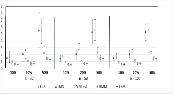
Figure 3.6:The Box plots exhibit how various proportions of outliers affect the mean (standard deviations) of the MSE values for the five proposed estimators (OLS, LMS, MM, BMM, and FBM) with different choices of
multiple sizes assuming the proposed marginal errors belongs to t distribution.
Figure 3.7:The Box plots exhibit how various proportions of outliers affect the mean (standard deviations) of the MSE values for the five proposed estimators (OLS, LMS, MM, BMM, and FBM) with different choices of
156
Figure 3.8:The Box plots exhibit how various proportions of outliers affect the mean (standard deviations) of the MSE values for the five proposed estimators (OLS, LMS, MM, BMM, and FBM) with different choices of
multiple sizes assuming the proposed marginal errors belongs to Uniform distribution.
4. Applications on Real Data
The most important thing in researches is the application side, because it's useful to solve many of practical problems, also application support the validation of our theoretical results obtained through simulations.
4.1 The Education and Related Statistics for the U.S. States
The Education data frame has 51 observations and 4 variables. The observations are collected from the U. S. states and Washington, D. C. This data can be easily obtained from the book of Statistical Abstract of the United States (Bureau of the Census, 1992). This data frame contains the following variables: At first, we compute the some statistical properties of the education data. Table 4.3 consists of the means and standard deviations of the four chosen variables that are formed the education data.
Table 4.1:Same statistical properties of the four variables that from the education Data (mean and standard deviation) SATM x1 Percent x2 Pay/$1000 x3 Dollar Y Min 437.0 4.00 22.00 2.993 1st Qu 470.0 11.50 27.50 4.354 Median 490.0 25.00 30.00 5.045 Mean 497.4 33.75 30.94 5.175 3rd Qu 522.5 57.50 33.50 5.690 Max 577.0 74.00 43.00 9.159 St. dev. 34.5688 24.0739 5.3081 1.3762 TheDurbinWatson=1.768
From table 4.1, we notice that the mean and median values of the explanatory variables x2 and x3 are pretty close
to each other. Whereas, the explanatory variables x1 have relatively larger mean and median values respectively.
157
close to each other. Whereas, the explanatory variables x3 has a smaller standard deviation value. This give
initial indication of having some values that might be outliers. Finally, the Durbin-Watson measure confirm no existence of the multicollinearity problem between the explanatory variables x1, x2 and x3 . Figure (4.1) display
the scatter plot of the dollars (y) with each one of the three explanatory variables.
Figure 4.1:The scatterplot of the three explanatory variables that from the Education.
Having a close look at the scatter plots in Figure 4.2, we notice the following remarks: Firstly, the plot of the variables SATM x1 versus the dependent variable Dollars (y) seem to have several outliers in xydirection.
Secondly, the plot of the variable Dollars (y) versus percentx2 seems to have several outliers in x-direction.
Thirdly, the plot of the variable Dollars (y) versus payx3 seems to have several outliers in xydirection. Overall,
we can conclude that the Education data does contain outliers. This means the response variable y must be explained through a mixture of explanatory variables. Next, we utilize the five different methods of handling the problem of the outliers (OLS, LMS, MM, BMM and FBM) for the dollars data. Table 4.4 contains the numerical summary of the fitted models (including the coefficients and the values of mean squared error).
10 20 30 40 50 60 70
3
4
5
6
7
8
9
percent 0.025 0.030 0.035 0.040 3 4 5 6 7 8 9 pay/1000440 460 480 500 520 540 560 580 3 4 5 6 7 8 9 SATM
158
Table 4.2: contains the numerical summary of the five proposed models applied on the Education Data.
β0 β1 β2 β3 OLS -6.39772895 0.01104814 0.03039559 0.16328591 LMS -6.7882534 0.01461188 0.03010912 0.10694682 MM -5.9758597 0.009962355 0.024686046 0.171564016 BMM -6.347148 0.01064757 0.02721239 0.17039220 FBM -6.321678 0.01055311 0.02490381 0.17257998
From Table 4.2,we notice several important points: Firstly, the FBM estimator provides the smallest value of
MSE followed by the BMM estimator. Whereas, the OLS estimator provides the largest value of MSE. Secondly, the MM estimator and LMS estimator also provides smaller MSE values comparing with the OLS
estimator, but not as good as the MSE values obtained by using the FBM estimator and the BMM estimator. Therefore, the analysis of the Education Data has proven that the FBM estimator is superior estimator followed by small margins the BMM estimator and this agreed once more with the results obtained from the simulation study.
5. Summary and Conclusion
From the simulation study, the estimated values of the mean squared errors (MSE) have supported that the superiority of the FBM estimator and trailed very closely by the BMM estimator, regardless to both the type of errors' distributions as well as with all possible sample sizes n, and in The linear regression case (p= 1 – 2, and 5). When the outliers are in Y- direction and inthe choices of the number of the explanatory variables were (p= 1, 2, and 5 ),we have noticed the following remarks:
1. the FBM estimator provides the smallest mean and standard deviation values of MSE followed by the BMM
estimator. Whereas, the OLS estimator provides the largest mean and standard deviation values of MSE, regardless to both the type of errors' distributions as well as with all possible sample sizes n. When the outliers are in X- direction and inthe choices of the number of the explanatory variables were ( p= 1, 2, and 5 ),we have noticed the following remarks:
1-the FBM estimator provides the smallest mean and standard deviation values of MSE followed by the BMM
estimator, regardless to both the type of errors' distributions as well as with all possible sample sizes n.
2-the OLS estimator provides the largest mean and standard deviation values of MSE, in the case of the marginal error terms belong to the t distribution and to the Exponential distribution.
Whereas, the LMS estimator provides the largest mean and standard deviation values of MSE, in the case of the marginal error terms belongs to the normal distribution and to the uniform distribution.
When the outliers are in XY- direction and in the choices of the number of the explanatory variables were ( p= 1, 2, and 5 ),we have noticed the following remarks:
159
1-the FBM estimator provides the smallest mean and standard deviation values of MSE followed by the BMM
estimator. Whereas, the OLS estimator provides the largest mean and standard deviation values of MSE, regardless to both the type of errors' distributions as well as with all possible sample sizes n.
Reference
[1] Beasley, D.A., Kuh, E., and Welsch, R.E (1980) Regression Diagnostics: Identifying Influential Data and sources of Collinearly. Wiley, New York.
[2] Birkes, D. and Dodge, Y (1993) Alternative Methods of Regression. New York: John Wiley and Sons.
[3] CHEN, C. (2002) Robust Regression and Outlier Detection with the ROBUSTREG procedure [online].
SUGI Paper, SAS Institute Inc., Cary, NC., http://www2.sas.com/proceedings/sugi27/p265-27.pdf
[4] Cleveland, W. S., and McGill, R. (1984). Graphical perception: Theory, experimentation, and application to the development of graphical methods. Journal of the American statistical association,
554 .- 531 (, 783)79
[50] COLE, S. R. (1999) Simple bootstrap statistical inference using the SAS system. Computer Methods and Programs in Biomedicine, 60, pp. 79–82.
[6] Cook, R.D. (1977) Detection of Influential Observations in Linear Regression. Techno metrics 19: p 15-18.
[7] DICICCIO, T. J., EFRON, B. (1996) Bootstrap confidence intervals. Statistical Science, 11(3), pp. 189– 212.
[8] Draper, N. R. and Smith, H (1998) Applied Regression Analysis. 3rd ed. New York: John Wiley & Sons.
[9] Efron, B. (1979). Computers and the theory of statistics: thinking the unthinkable. SIAM review, 21(4), 460-480.
[10] Efron, B., and Tibshirani, R. J. (1993). CHAPMAN&HALL/CRC (Eds.), An Introduction to the Bootstrap. New York, U.S.A.
[11] Fan, J., and Gijbels, I. (1996). Local Polynomial Modelling and its Applications. London: Chapman & Hall.
[12] Fox, J. (1997) Applied Regression Analysis ,Linear Models, and Related Methods . Sage Publications.
160
[14] FREEDMAN, D. A. (1981) Bootstrapping regression models. The Annals of Statistics, 9(6), pp. 1218– 1228.
[15] Galton, F. (1886). Regression towards mediocrity in hereditary stature. The Journal of the Anthropological Institute of Great Britain and Ireland, 15, 246-263.
[16] Jaber, A. M. (2008) On using Robust Regression. Unpublished
[17] M.Sc. Thesis, University of Benghazi, Benghazi, Libya.
[18] Huber, P. J, (1964)." Robust Estimation of a Location parameter. Annals of Mathematical Statistics 35:73, 101
[19] Huber, P. J. (1981) Robust statistics. New York: John Wiley and Sons.
[20] HUBERT, M., ROUSSEEUW, P. J., and VAN AELST. (2008) High-Breakdown Robust Multivariate Methods. Statistical Science, , 23(1), pp. 92–119.
[21] Kutner, M. H., Nachtsheim, C., and Neter, J. (2004). Applied linear regression models. McGraw-Hill/Irwin.
[22] Kleinbaum, D. G., Kupper, L. L., Muller, K. E. and Nizam, A. (1998) Applied Regression Analysis and Other Multivariable Methods. California: Duxbury Press.
[23] Lane, K. (2002). What is robust regression and how do you it?, the Annual Meeting of the South Educational Research Association, Austin, Texas ED 466-697 P:15.
[24] Olive, D.J. (2007) Applied Robust Statistics. Southern Illinois University Department of Mathematics.
[22] Rahmatullah Imon, A.H.M. (2007).Cited at http://mnt.math.um.edu.my/ismweb/Announcement/Imon PG3.pdf
[26] Rousseeuw, P. J. and Leroy, A. M. (1987) Robust Regression and Outlier Detection. New York: John Wiley and Sons.
[27] ROUSSEEUW, P. J., LEROY, A. M.(2003) Robust Regression and Outlier Detection. John Willey and Sons , New Jersey, USA.
[28] Ruppert, D., and Carroll, R. J. (1980). Trimmed least squares estimation in the linear model. Journal of the American Statistical Association, 75(372), 828-838.
[29] Stine, R. (1990). An introduction to bootstrap methods: examples and ideas. In Fox, J. and Long, J. S., editors, Modern Methods of Data Analysis, pages 325{373. Sage, Newbury Park, CA.