Feature-based Time Series Analytics
Dissertation
zur Erlangung des akademischen Grades Doktoringenieur (Dr.-Ing.)
vorgelegt an der
Technischen Universität Dresden Fakultät Informatik
eingereicht von
Dipl.-Inf. Lars Kegel
geboren am 16. Juni 1988 in Dresden
Gutachter: Prof. Dr.-Ing. Wolfgang Lehner Technische Universität Dresden Fakultät Informatik
Institut für Systemarchitektur Lehrstuhl für Datenbanken 01062 Dresden
Prof. Themis Palpanas University of Paris LIPADE
45, rue des Saints-Pères 75006 Paris
Frankreich Tag der Verteidigung: 9. März 2020
ABSTRACT
Time series analytics is a fundamental prerequisite for decision-making as well as au-tomation and occurs in several applications such as energy load control, weather re-search, and consumer behavior analysis. It encompasses time series engineering, i.e., the representation of time series exhibiting important characteristics, and data mining, i.e., the application of the representation to a specific task. Due to the exhaustive data gathering, which results from the “Industry 4.0” vision and its shift towards automation and digitalization, time series analytics is undergoing a revolution. Big datasets with very long time series are gathered, which is challenging for engineering techniques. Tradition-ally, one focus has been on raw-data-based or shape-based engineering. They assess the time series’ similarity in shape, which is only suitable for short time series. Another focus has been on model-based engineering. It assesses the time series’ similarity in structure, which is suitable for long time series but requires larger models or a time-consuming modeling. Feature-based engineering tackles these challenges by efficiently representing time series and comparing their similarity in structure. However, current feature-based techniques are unsatisfactory as they are designed for specific data-mining tasks.
In this work, we introduce a novel feature-based engineering technique. It efficiently pro-vides a short representation of time series, focusing on their structural similarity. Based on a design rationale, we derive important time series characteristics such as the long-term and cyclically repeated characteristics as well as distribution and correlation char-acteristics. Moreover, we define a feature-based distance measure for their comparison. Both the representation technique and the distance measure provide desirable properties regarding storage and runtime.
Subsequently, we introduce techniques based on our feature-based engineering and ap-ply them to important data-mining tasks such as time series generation, time series match-ing, time series classification, and time series clustering. First, our feature-based genera-tion technique outperforms state-of-the-art techniques regarding the accuracy of evolved datasets. Second, with our features, a matching method retrieves a match for a time series query much faster than with current representations. Third, our features provide discrim-inative characteristics to classify datasets as accurately as state-of-the-art techniques, but orders of magnitude faster. Finally, our features recommend an appropriate clustering of time series which is crucial for subsequent data-mining tasks. All these techniques are assessed on datasets from the energy, weather, and economic domains, and thus, demon-strate the applicability to real-world use cases. The findings demondemon-strate the versatility of our feature-based engineering and suggest several courses of action in order to design and improve analytical systems for the paradigm shift of Industry 4.0.
CONTENTS
1 INTRODUCTION 11
2 FOUNDATIONS OF TIME SERIES ANALYTICS 15
2.1 Time Series and Domains . . . 15
2.1.1 Time Series in Energy . . . 16
2.1.2 Time Series in Meteorology and Climate . . . 17
2.1.3 Time Series in Medicine . . . 18
2.2 Data-mining Tasks . . . 18
2.2.1 Time Series Generation . . . 19
2.2.2 Time Series Matching . . . 19
2.2.3 Time Series Classification . . . 19
2.2.4 Time Series Clustering . . . 20
2.3 Challenges. . . 20
2.4 Summary . . . 21
3 TIME SERIES ENGINEERING 23 3.1 Raw-data-based Engineering . . . 24 3.2 Shape-based Engineering . . . 26 3.2.1 Representation . . . 26 3.2.2 Distance . . . 28 3.3 Model-based Engineering . . . 29 3.3.1 Representation . . . 30 3.3.2 Distance . . . 35 3.4 Feature-based Engineering . . . 36 3.4.1 Representation . . . 36 3.4.2 Distance . . . 39 3.5 Summary . . . 39
4 FEATURE-BASED ENGINEERING ACROSS DATA-MINING TASKS 41 4.1 Design Rationale . . . 42
4.2 Time Series Model . . . 43
4.3 Decomposition . . . 43
4.3.1 Related Work . . . 44
4.3.2 Multi-seasonal Decomposition . . . 44
4.4 Feature-based Representation . . . 45
4.4.1 Features for Deterministic Components . . . 46
4.4.2 Features for Stochastic Component . . . 47
4.4.3 Representation Size . . . 47
4.4.4 Representation Time . . . 48
4.5 Feature-based Distance Measure . . . 49
4.6 Summary . . . 50
5 TIME SERIES GENERATION 51 5.1 State of the Art . . . 52
5.1.1 Properties of Generation Techniques. . . 52
5.1.2 Raw-data-based Generation Techniques. . . 53
5.1.3 Model-based Generation Techniques . . . 54
5.1.4 Assessing Expressiveness. . . 56 5.1.5 Comparison . . . 57 5.2 Feature-based Generation . . . 58 5.2.1 Feature-based Modification . . . 58 5.2.2 Feature-based Recombination . . . 60 5.2.3 Comparison . . . 64 5.3 Experimental Evaluation . . . 64 5.3.1 Experimental Setting . . . 65 5.3.2 Feature-based Distance . . . 66 5.3.3 Standard Distance . . . 68 5.4 Summary . . . 71
6 TIME SERIES MATCHING 73 6.1 State of the Art . . . 74
6.1.1 Original SAX . . . 75
6.1.2 SAX Extensions . . . 76
6.2 Season- and Trend-aware Symbolic Approximation . . . 77
6.2.1 Season-aware Symbolic Approximation . . . 78
6.2.2 Trend-aware Symbolic Approximation . . . 81
6.2.3 Properties of Engineering Techniques . . . 83
6.3 Experimental Evaluation . . . 83
6.3.1 Experimental Setting . . . 84
6.3.2 Results and Discussion . . . 87
6.4 Summary . . . 91
7.1 State of the Art . . . 94
7.1.1 Run Length Distribution . . . 95
7.1.2 Discrete Wavelet Transform . . . 95
7.1.3 Large Feature Vector . . . 96
7.2 System Overview . . . 96 7.2.1 Labeled Dataset . . . 97 7.2.2 Feature-based Representation . . . 97 7.2.3 Normalization . . . 98 7.2.4 Feature Selection . . . 99 7.2.5 Feature-based Classification . . . 99 7.3 Experimental Evaluation . . . 100 7.3.1 Experimental Setting . . . 100
7.3.2 Results and Discussion . . . 103
7.4 Summary . . . 108
8 TIME SERIES CLUSTERING 109 8.1 Cross-sectional Autoregression Model . . . 110
8.1.1 Integration . . . 110
8.1.2 Autoregression . . . 111
8.1.3 Error Terms . . . 111
8.2 Feature-based Clustering. . . 112
8.2.1 ACF and PACF for ARIMA . . . 112
8.2.2 ACF and PACF for CSAR . . . 112
8.3 Experimental Evaluation . . . 113
8.3.1 Experimental Setting . . . 113
8.3.2 Results and Discussion . . . 116
8.4 Summary . . . 118
9 CONCLUSIONS 119 BIBLIOGRAPHY 123 LIST OF FIGURES 133 LIST OF TABLES 135 A PROOFS FOR SSAX AND TSAX 137 A.1 Proof of Lower-bounding sPAA. . . 137
A.2 Proof of Lower-bounding sSAX . . . 139
A.3 Proof of Combined Trend Feature . . . 140
A.4 Proof of Lower-bounding tPAA. . . 140
A.5 Proof of Lower-bounding tSAX . . . 141
B LIST OF SYMBOLS 143
ACKNOWLEDGMENTS
First and foremost, I would like to thank Wolfgang Lehner for giving me the opportunity to realize this thesis project. As my advisor, he guided my research project, provided many ideas as well as valuable feedback. He also gave me the time and freedom I needed to evolve my thesis plan. Because of him, I was able to attend exciting conferences and workshops and to gain experience with industrial partners. Thanks for everything! I want to thank Themis Palpanas for co-refereeing this thesis. Moreover, I am deeply grateful to my colleagues Claudio Hartmann and Martin Hahmann, who acted as co-advisors over the last years. Claudio took a lot of time for discussions concerning my research, as he is also deeply interested in time series analytics. He was also a great roommate and created a productive working atmosphere. I am also thankful for our co-operation in time series forecasting and clustering. Martin offered me a lot of support in publishing papers, especially in finding an appealing and convincing writing style. With his great sense of humor, he enriched every conversation, and I am looking forward to his conference on surreal computer sciences. I also want to thank my former supervisors, who inspired me with their work on time series analytics while I was studying: Philipp Rösch and Lars Dannecker from SAP, and especially Ulrike Fischer.
This thesis would not have been possible without the support from the team. I am thank-ful to all my colleagues for a great and creative atmosphere that included constructive discussions as well as fun coffee breaks. Thank you, Alex, Annett, Axel, Dirk, Elvis, Jo-hannes P., JoJo-hannes L., Julius, Lisa, Maik, and Patrick! Special thanks also to Robert and Lucas for many fruitful collaborations on student courses and theses. I am deeply grate-ful to Ioana Manolescu, who provided me “academic shelter” for one year; her research group, especially Alexandre, Félix, Khaled, Maxime, Mikaël, Mirjana, Paweł, and Tayeb, received me well, and I enjoyed the social activities. A special thanks to all students who contributed to my research projects. Moreover, I would like to thank Claudio, Jiˇri, and Olga for proof-reading this thesis and for providing many valuable comments.
Finally, I am deeply grateful for the constant encouragement from my family and friends. My parents Ilona and Lutz, as well as my sister Anita always stood behind me and sup-ported me during this tough time. Moreover, I enjoyed unforgettable activities with my friends and band. The music we played did not only made our audience happy; it also made me happy. Thank you for helping me keep a work-life balance!
Lars Kegel Dresden, January 9, 2020
1
INTRODUCTION
E
XHAUSTIVE DATA GATHERINGis not a new trend anymore but can be considered stan-dard practice in many domains. It is the primary driver of the current paradigm shift in industrial production towards automation and digitalization. Especially the German-speaking area refers to this shift asIndustry 4.0 [LFK+14]. For example, smart factoriesfollow this paradigm shift; they are heavily equipped with sensors providing informa-tion to autonomous factory systems. Besides, parameters ofcyber-physical systems, which merge physical and digital components, are monitored for controlling and maintenance. Finally, systems connected via theInternet of Things(IoT) monitor and communicate their status [XYWV12].
A significant part of these measured values is captured over time and thus forms a time series [SS11]. A dataset of these time series gives analytical insights into the underly-ing processes, which are uncovered by data minunderly-ing. Four insights are fundamental for this work: the extraction of important time series characteristics and their reproduction [MS82], the retrieval of a similar time series [AFS93], the mapping of a time series to a class label [PO94], and the partitioning of a dataset into meaningful clusters [Bel77]. We refer to these four data-mining tasks as time series generation, time series match-ing, time series classification, and time series clustermatch-ing, respectively. In recent years there has been growing interest in carrying out these data-mining tasks in many domains [KHL18, ZP18, BLB+17, ASY15].
It is challenging to carry out these data-mining tasks for two reasons. First, time series are inherently high-dimensional. Their discriminative characteristics do not arise from one single value, but from many, possibly very distant values. Moreover, these character-istics do not only appear by considering each value in isolation, but also from the mutual dependence of values. Since data-mining tasks usually focus on low-dimensional data types, they are not directly applicable to time series and their specific nature. Second, exhaustive data gathering leads to big datasets. Not only do time series occur together with thousands of other time series, but they also have a fine granularity, leading to large series with tens of thousands of values. Thus, they require much storage, and their com-parison is time-consuming. Overall, techniques are required that transform time series in a low-dimensional representation, while enabling effective and efficient data mining. In the literature, the termengineeringrefers to the branch of science and technology that focuses on the design, the building, and the use of structures [Lex19]. With this in mind, we introduce the termtime series engineeringto refer to the task of designing a representa-tion techniquethat builds a low-dimensionalrepresentationof a time series and of design-ing adistance measurewhich describes how far away two representations are by returning
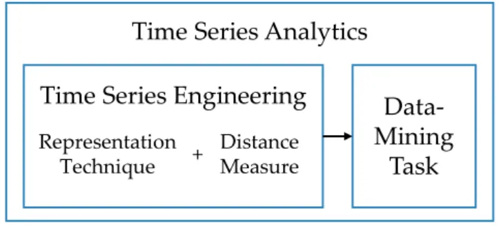
Time Series Analytics
Time Series Engineering
Data-Mining Task
Representation
Technique + DistanceMeasure
Figure 1.1: Time Series Analytics
theirdistance(Figure 1.1). Thus, time series engineering provides techniques to transform a time series into a low-dimensional representation, exhibiting its important characteris-tics. Consequently, the termtime series analyticsencompasses time series engineering and the application to a data-mining task.
The energy, meteorological, and economic domain are attracting considerable interest due to the rise of cyber-physical systems and IoT, and we focus on them in our research projects [FFQ17, GOF17]. In the energy domain, a multitude of smart meters and en-ergy management systems captures processes as time series, such as the electricity con-sumption in households and businesses. This data is gathered by the grid operator and provides analytical insights to control the load in the grid [UFLD13]. Meteorological time series are heavily analyzed to assess the feasibility of industrial installations, such as wind or solar power plants [MS82]. Besides, climate phenomena are also captured as time series. For example, they provide insights about dependent ecosystems [STK+03].
In the economic domain, macro-economic, sales, and payment data is gathered as time series and analyzed for better decision-making [MSA18]. For example, many shops mon-itor payment transactions to analyze and forecast consumer behavior [Int17]. Since these domains also face the challenges of big datasets it is of highest importance to apply a suitable engineering technique to capture the important characteristics of these datasets. There is a considerable amount of literature on engineering techniques. While raw-data-based techniques focus on the time series as is, applying different measures to describe their distance, shape-based and model-based techniques reduce a time series to a low-dimensional space, by selecting important points, aggregating segments of the time se-ries, or estimating a generative model.
Feature-based techniques form the fourth class of engineering techniques. A feature is a global time series property, which arises from the application of a method from the time-series analysis literature [FLJ13]. These features are gathered as a feature vector, characterizing a time series by its important characteristics. This class of engineering techniques is very promising for big datasets, as it focuses on global structural properties and calculates them efficiently. As such, different feature-based techniques have been applied to various data-mining tasks, such as generation, matching, classification, and clustering. However, they cannot be easily adopted by other data-mining tasks, as they do not support their specific requirements. A generation technique must evolve new time series from a representation, while a classification technique requires discrimina-tive features for accurately mapping time series to their correct class label. Time series matching requires a distance measure for an efficient retrieval, while clustering relies on a distance measure for grouping similar time series and separating dissimilar ones. These requirements have not yet been addressed altogether.
With this in mind, our goal is the design of a feature-based engineering technique that is used across data-mining tasks. First, it has to capture important characteristics of time
series. Second, it should provide desirable properties regarding space and runtime, i.e., it should efficiently build a short representation and compare them with an efficient dis-tance measure, and thus, tackle the challenges of big datasets. Finally, it should consider specific requirements from data-mining tasks and provide analytical insights effectively and efficiently.
Summary of Contributions
Overall, we propose a feature-based engineering technique that efficiently captures the long-term and cyclically repeated characteristics of a time series in a short representation, together with its distribution and correlation characteristics. Its distance measure focuses on the global structural similarity, which is desirable for big datasets with long time series [WSH06]. Moreover, we show its versatility to handle fundamental data-mining tasks. In more detail, the contributions of this work are:
• We give an overview of domains where time series analytics plays an important role, and exemplify data-mining tasks on three selected domains. Moreover, we motivate time series engineering by formulating the challenges of data-mining tasks regarding big time series datasets.
• We survey engineering techniques from the literature and review them regarding desirable properties for the application on big time series datasets. We conclude that a versatile feature-based technique is required to tackle a variety of data-mining tasks.
• We introduce a feature-based engineering technique, which applies to a multitude of domains and across data-mining tasks. Moreover, we demonstrate its competi-tive properties compared to other techniques [KHL17b, KHL18].
• We give an overview of time series generation by surveying generation techniques and comparing the characteristics they are able to reproduce. Moreover, we propose feature-based generation techniques that reproduce these characteristics accurately [KHL16, KHL17a, KHL18].
• We extend the state-of-the-art engineering technique for time series matching, the symbolic aggregate approximation [LKLC03], with features from our engineering technique, which leads to a significantly more effective and efficient matching with-out increasing the representation size.
• Regarding time series classification, we survey engineering techniques for the clas-sification of long time series. Taking into account both effectiveness and efficiency, we propose a feature-based classification that classifies as accurately as state-of-the-art techniques, but orders of magnitude faster.
• We assess a feature-based clustering of a dataset, applied to time series forecasting. In particular, we show that a vectorized forecast technique [Har18], estimating one model for a cluster of time series, is more accurate if the time series in a cluster have similar features [HKL20].
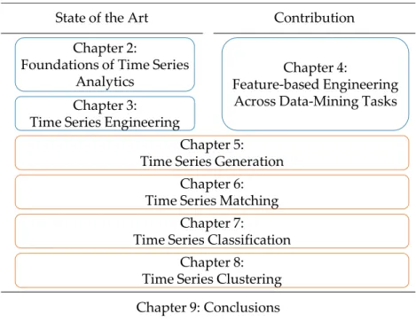
State of the Art Contribution
Chapter 9: Conclusions
Chapter 4:
Feature-based Engineering Across Data-Mining Tasks Chapter 2:
Foundations of Time Series Analytics
Chapter 5: Time Series Generation
Chapter 6: Time Series Matching Chapter 3:
Time Series Engineering
Chapter 7:
Time Series Classification Chapter 8:
Time Series Clustering
Figure 1.2: Structure of this Work Structure of this Work
Figure 1.2 illustrates the overall structure of this work. In the first part, we give the nec-essary background on time series engineering. Chapter 2 starts with the foundations of time series analytics by giving example applications of time series and by explaining the challenges of data mining. Chapter 3 surveys engineering techniques for time se-ries. Based on these observations, we introduce our engineering technique in Chapter 4 along with a feature-based representation technique and distance measure. In the second part, we shift our attention to four selected data-mining tasks, i.e., time series genera-tion (Chapter 5), time series matching (Chapter 6), time series classificagenera-tion (Chapter 7), and time series clustering (Chapter 8). We start each of these chapters by introducing state-of-the-art engineering techniques and desirable properties. Subsequently, we apply our engineering technique to the data-mining task and evaluate it experimentally. We fi-nally conclude this work in Chapter 9 with a summary and challenges for future research activities.
2
FOUNDATIONS OF TIME SERIES ANALYTICS
T
HIS CHAPTERgives an overview of time series analytics. It introduces time series as the fundamental data type for this work and identifies domains that gather this data for different purposes (Section 2.1). Subsequently, it presents data-mining tasks for time series and exemplifies the relevance of four data-mining tasks, time series generation, matching, classification, and clustering in several domains (Section 2.2). Finally, it identi-fies challenges of big time series datasets, which lead researchers to carry out time series engineering (Section 2.3). We conclude with a summary of our observations (Section 2.4).2.1
TIME SERIES AND DOMAINS
It is quite natural in many domains to measure a process at consecutive time instances. The measured values are likely to depend on each other instead of being independent and identically distributed [SS11]. The data type that stores measured values is atime series. It covers thevalue domainby storing each value as a real number, and it covers the time domainby storing the values in increasing order of time. Formally, a time seriesyis a vector of valuesythat are measured at discrete time instancest:
y|= (y1,..., yt,..., yT)wherey∈RT, t∈N>0, t≤T (2.1)
The distance between two time instances is calledgranularity. In this work, we assume that a time series (1) is finite with a fixed lengthT, (2) is complete, i.e., there are no missing values, and (3) is equidistant, i.e., the distance between between any two consecutive time instances is constant. Works that omit these conditions, i.e., omit condition (1) and process time series in a streaming fashion or omit conditions (2) and (3) and process irregular time series, are orthogonal and not covered in this work. Conditions (2) and (3) are achieved by cleaning and transforming the data beforehand.
Often, processes that are related to each other are bundled together. Consequently, they are stored as atime series datasetwhich is a set ofI time series:
Y ={y1,..., yi,..., yI}wherei∈N>0, i≤I (2.2) where we assume that all time series of a dataset have the same length.
There is a multitude of domains that use time series for data mining [SS11, Fis14]. As shown in Figure 2.1, they may be broadly categorized into four groups:Economy, Inani-mate Nature and Environment,Biometrics, andSociety.
Economy Computing · online advertisement · query processing Energy · energy balancing · gas production Finance · stock development · price development Industry · production planning · inventory planning Sports · player performance · team performance Tourism · tourist visits · airline passengers Inanimate Nature and Environment Biometrics Society Chemistry · chemical concentration
Meterology & Climate
· wind speed and direction · climate index Physics · sunspots · earthquakes Remote Sensing · deforestation · desertification Agriculture · animal population · yield Epidemiology · Influenza cases Medicine · electrocardiography · magnetic resonance imaging
Crime · robberies · drunkenness Demography · population rate · immigrants Macro-Economy
· gross national income · inflation
Politics
· election outcome · unemployment rate
Figure 2.1: Domains of Time Series
The first group, Economy, encompasses domains such as computing, energy, finance, industry, sports, and tourism. These domains utilize time series for market research and for supporting business processes. The energy domain is attracting widespread interest due to the increased installations of smart metering and energy management systems that measure many electric processes at a fine granularity for energy load control. Therefore, we give a brief overview of two data-mining tasks in this domain (Subsection 2.1.1). In the second group, Inanimate Nature and Environment, researchers study the natural sciences (chemistry, physics), and environmental sciences (meteorology and climate, re-mote sensing). In these domains, time series express natural and environmental phenom-ena over time and allow decision-makers to take actions such as planning new industrial sites or adopting new environmental policies. In meteorology and climate, big time series datasets that contain weather and climate influences are most interesting for an analysis, which is why we give an overview of data-mining tasks in this domain (Subsection 2.1.2). Biometrics is the application of statistical analysis to biological data. It encompasses do-mains such as agriculture, epidemiology, and medicine. In medicine, time series support medical diagnosis and data-mining tasks are among the most commonly discussed in the literature, which is why we present three data-mining tasks from this domain (Subsection 2.1.3).
The last group, Society, studies the social sciences and social relationships. It encom-passes domains such as crime, demography, macro-economy, and politics. For example, demography utilizes time series for grouping societies with similar development of their population. These insights are used by decision-makers for adopting new policies. Subsequently, we present scenarios from three selected domains, energy, meteorology and climate, as well as medicine, and demonstrate the use of time series for their pur-poses.
2.1.1 Time Series in Energy
By 2020, the European Union aims at producing at least 20% of its total energy using re-newable energy sources (RES) [Eur09], and by 2030, it has even higher ambitions [Eur19]. The impact of RES on the electricity sector is the highest compared to other sectors
[Eur19]. However, the feed-in of RES is challenging due to their intermittent and irregu-lar nature. Soirregu-lar power is produced only during the day and not during the night while, in Germany, wind energy is produced mostly in winter. The energy production is more and more decentralized, but the existing grid was initially designed for unidirectional power flows, i.e., from power plants to consumers.
To tackle these challenges, several technologies have been proposed that are innovated and rolled out piece by piece. Among them, smart meters and data management plat-forms contribute to a balanced energy grid, and they do this by time series analytics. Smart meters record and transmit the energy consumption of a household, a circuit, or a device to improve energy savings. One approach is to notify a consumer about the cor-rect, inefficient, or even faulty behavior of a device and recommend him to take action. Thus, the monitored device is the process whose measured values are captured as a time series. A classification model is trained to identify a device and its behavior automati-cally [LBCSA11]. Grid authorities may also store time series from smart meters on a data management platform. On this aggregated level, they use time series to provide better analytical insights and to balance the energy grid [UFLD13]. Moreover, they have to take care that the data management platform fulfills the specific requirements of their area, i.e., the correct sizing and performance. Therefore, Arlitt et al. propose an assessment tool that involves time series generation. This tool helps grid authorities to assess their data management platform by loading and analyzing generated datasets with realistic characteristics, but configurable in their size [AMB+15].
Thus, we identify time series classification and generation as crucial data-mining tasks in the energy domain.
2.1.2 Time Series in Meteorology and Climate
Meteorological time series capture a variety of atmospherical phenomena such as tem-perature, solar irradiation, wind speed, wind direction, and precipitation. They are most frequently used for estimating weather prediction models that provide forecasts of these phenomena. Besides forecasting, these time series are also used in two other data-mining tasks, which are time series generation and time series clustering.
Systems that rely on atmospherical phenomena have to be assessed in order to test and verify their performance, their robustness, and their correct sizing. For example, wind power plants are heavily evaluated for possible weather scenarios (wind speed and wind direction at different altitudes) before they are installed at a specific location. If such scenario datasets are not available because measuring in the field is expensive or not possible, time series with realistic characteristics are generated [MS82].
An essential task in climate research is the discovery of climate phenomena linked to each other. These so-called teleconnections give explanations on how climate changes and how ecosystems respond to remote phenomena. Usually, they are discovered by climate indices capturing the variance on a regional and global level as a time series. It has been shown that clustering climate indices are an essential tool of discovering teleconnections [STK+03].
Anomaly Detection Classification Clustering Forecasting
Generation Matching Motif Discovery Subsequence Matching
Figure 2.2: Data-mining Tasks
2.1.3 Time Series in Medicine
In medicine, diagnostic tools capture a variety of characteristics from the human body. Two prominent examples are the electrocardiography (ECG) of the heart and the sequen-tial analysis of the deoxyribonucleic acid (DNA).
The ECG measures the heartbeat of a patient by its electrical activity. The values repre-sent time series that allow physicians to identify heart arrhythmia, i.e., conditions that result from disturbances of the heartbeat. Since some arrhythmias appear infrequently, patients have to be monitored over several days. Subsequently, physicians analyze the resulting time series, which can be very time-consuming. Therefore, research focuses on the automatic classification to support this task [DOR04].
Another diagnostic tool for medical but also for biological research is the sequential anal-ysis of the DNA, i.e., the determination of the nucleotides adenine, guanine, cytosine, and thymine in their sequential order. It enables researchers to discover homologies between species such as humans and monkeys. Since the DNA is very long and split into several chromosomes, it is a challenging task to match subsequences to each other in order to discover these homologies. Camerra et al. propose an approach where they translate a DNA sequence into real numbers forming a time series [CPSK10]. They build a time se-ries index that stores representations of all subsequences of a monkey DNA. Then, they query the index with subsequences from human DNA and find matches. These matches establish a co-occurrence map identifying the chromosomes of humans and monkeys that are most similar. Not only do their results agree with previous research, their time series index is also an efficient matching method.
Thus, time series classification and matching are crucial data-mining tasks in medicine.
2.2
DATA-MINING TASKS
Time series have been used in several data-mining tasks, as presented in Figure 2.2. Anomaly detection,clustering,generation,matching,motif discovery, andsubsequence matching are descriptive tasks, which analyze past and current data in order to prepare informed decisions. Classificationandforecastingare predictive tasks; they infer the class of an un-labeled time series and the future values of a given time series, respectively. Based on the examples mentioned above and their requirements, we focus on four selected data-mining tasks, explain and motivate them in the following subsections.
2.2.1 Time Series Generation
Time series generation extracts important characteristics from a given dataset and re-produces them in a generated dataset. While this looks like a paradox considering the abundance of data that is collected, it is still a very important task for evaluating a system and for providing evolved data in case there is no given data available.
Thus, it has been applied in a multitude of domains. As reported earlier, it is used in the meteorological domain for generating wind speed time series [MS82]. Since then, researchers have been developing techniques for simulating further weather parameters [JL86, KKD91, BdMK02, MH15]. The energy domain utilizes it to assess renewable energy power plants [JL86, ILD+17], while industry and computing apply generated datasets for
various evaluation purposes [CDB94, SJ13].
2.2.2 Time Series Matching
Time series matching retrieves a time series from a dataset that is most similar to a query time series [KK03]. A naive matching algorithm compares the query time series to each time series from the dataset one by one. However, this approach is time-consuming which is why matching methods focus on a more efficient retrieval. Efficiency can be increased by pruning unpromising observations as early as possible [AFS93].
The data-mining task was first mentioned in 1993 where Agrawal et al. presented an R*-index that stores coefficients of the Fourier transform of time series [AFS93]. It gained popularity by the GEMINI approach (GEneric Multimedia INdexIng) where researchers built upon their work on time series engineering [Fal96, KK03]. Since then, progress has been made towards an effective and efficient time series engineering [LKLC03], i.e., a better pruning and a faster distance calculation, and towards more efficient indexing structures [SK08]. Up to now, index structures are improved regarding build time and contiguity [CPSK10, KDZP18].
Time series matching is widely applied in domains such as industry, finance [AFS93], and medicine. The matching of DNA sequences is a prominent example [CPSK10].
2.2.3 Time Series Classification
Time series classification is a supervised data-mining task that maps an unlabeled time series to a class label [KK03]. It is applied for two reasons: to support human classification decision [DOR04] and to fully automatize processes by, for example, triggering events in case of irregular time series [PO94].
Usually, classification is carried out for observations from a low-dimensional space. How-ever, time series are high-dimensional and their values are mutually dependent [KK03]. Due to these differences, time series classification may considered a proper data-mining task. As such, it was first discussed in an automated labeling of control charts in 1994 [PO94]. It gained more attention as researchers started proposing highly discrimina-tive distance measures that classified their datasets well [KK03]. Up to 2017, researchers also focused on better time series engineering and on combining classification techniques [BLB+17].
Following Chen et al. [CKH+15], classification problems mainly arise from computing
where signals from images, sensors, and motions are observed, from medicine where the automated labeling of the aforementioned ECG signals but also of, e.g., blood flow dynamics support the diagnosis, and from energy where electrical devices are classified by their signal in order to detect failures.
2.2.4 Time Series Clustering
Time series clustering is an unsupervised data-mining task. Its goal is to partition a time series dataset into clusters such that each cluster is homogeneous, i.e., the distance of time series within a cluster is minimal, while the distance of time series from different clusters is maximal [Lia05]. As pointed out in [ASY15], there are several reasons to carry out this data-mining task. (1) Clusters may uncover interesting patterns in a dataset, thus they help to identify frequent patterns that arise commonly as well as suprising patterns that arise rarely. (2) Clustering supports the exploration of big time series datasets by partitioning big datasets and presenting only a prototype time series per cluster. More-over, these clusters s may be hierachically ordered such that they may be collapsed and uncollapsed. (3) It is applied as a subroutine in other data-mining tasks such as time series forecasting. (4) The visualization of cluster structures helps to quickly understand the structure of the data along with its regular and irregular behavior.
Due to the special structure of time series, time series clustering is considered a proper data-mining task. Most often, clustering techniques are applied in a low dimension, too. However, time series engineering is necessary in order to prepare a dataset such that it presents the important characteristics to the clustering technique [Lia05].
Time series clustering was first mentioned in a work in 1977 [Bel77]. Since then, the data-mining task gained more and more attention because different techniques of time se-ries engineering were proposed and different clustering algorithms were applied [Lia05, ASY15]. Moreover, it is utilized in a multitude of domains. Among them, it has been applied in the climate domain to discover the aforementioned climate indices [STK+03],
in the energy domain to discover similar energy consumption behavior [KB90], and in medicine to partition ECG data [PG15].
2.3
CHALLENGES
Data-mining tasks for time series have to tackle two major challenges. First, they have to take many values into account that are ordered by time because a time series is an inherentlyhigh dimensionaldata type. Second, the paradigm shift of Industry 4.0 leads to an increasing number of sensors, and these processes are captured at a finer granularity. Thus, data-mining tasks facebig time series datasets. Subsequently, these two challenges are further detailed.
High Dimensionality
It is easier to carry out data-mining tasks once on a whole time series rather than once per time instance. The latter case would require to study the evolution of data-mining results across the time instances [Bel77]. Therefore, most publications focus on the former case and present whole time series to a data-mining technique, i.e., they present high-dimensional data.
One challenge arising from this presentation is theordering of the values by time. The important characteristics of a time series do not only arise by considering each value in isolation but also from the mutual dependence of values. Distance measures have to de-scribe this dependence accurately [KK03]. Besides the ordering, thelengthof a time series is a second challenge. Standard distance measures used for low-dimensional data cannot be effectively applied to long time series because the noise in the time series disturbs their results [KK03], and their notion of similarity becomes dubious [WSH06].
Data-mining tasks that take time series as is and that rely on standard distance measures become intractable: (1) Generation techniques aim at evolving time series that are similar to given time series regarding their shape, their value distribution, and their correla-tion [BdMK02]. Standard distance measures do not describe distribucorrela-tion and correlacorrela-tion characteristics and thus fail to provide this similarity. (2) Indexes for matching time se-ries cannot handle more than 16-20 dimensions, i.e., time sese-ries values. Time sese-ries are usually much longer and the index would degenerate [LKLC03]. (3) Time series classi-fiers could be prepared to work in a high-dimensional space. However, authors suggest reducing a time series rather than constructing complex classifiers [BDHL12]. (4) Some clustering techniques cannot handle high-dimensional data and would not accomplish their task on time series datasets [WSH06]. It is thus beneficial for these data-mining tasks to reduce the dimensionality of time series.
Big Time Series Datasets
Besides the high dimensionality, time series datasets are challenging due to their size. Once datasets are too big to fit into memory, data-mining tasks decrease in speed due to much disk I/O [ASY15]. Therefore, time series matching methods represent time series in a compressed manner so that they fit into memory. Due to pruning strategies, disk I/O is further reduced [LKLC03]. Other data-mining techniques such as highly accurate classifiers fail due to their complexity [BLHB15]. Clearly, they are not feasible for time series with a fine granularity.
2.4
SUMMARY
Although time series occur in many domains and provide insights for different purposes they are challenging due to their inherent nature and due to the increasing dataset size. Thus, data-mining tasks cannot be effectively and efficiently applied to provide analytical insights. These observations suggest that time series should be transformed in order to expose their important characteristics in a small representation.
3
TIME SERIES ENGINEERING
E
NGINEERING TECHNIQUES consist of two components: first, a representationtech-nique that builds representations of time series datasets and second, a distance mea-sure that uses representations to compare time series with each other. They tackle the challenges of big time series datasets for the following reasons. A representation tech-nique reduces a time series to a low-dimensional space and thus, a time series dataset has a smaller memory footprint. It provides representations that capture important char-acteristics. The distance measure ensures that these representations are similar if the original time series are similar [ASY15]. Moreover, the distance calculation is faster on a representation than on the original time series.
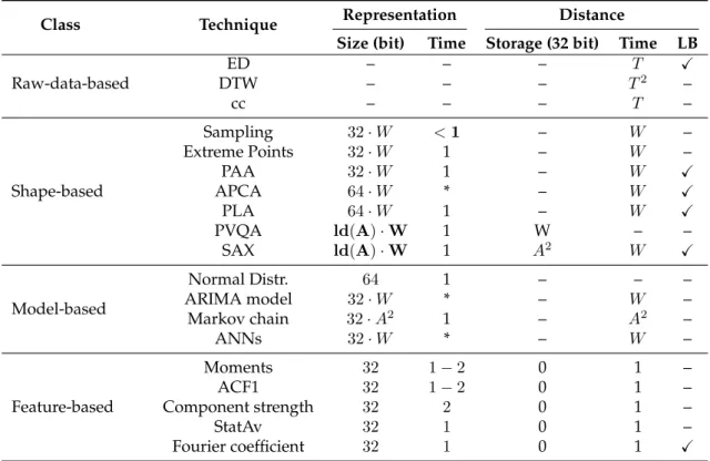
Figure 3.1 gives an overview of engineering techniques that are commonly applied in the literature. They are classified intoraw-data-based,shape-based,model-based, and feature-basedapproaches. While raw-data-based and shape-based engineering focuses on a sim-ilarity in shape, i.e., on a similarity of time-dependent characteristics, model-based and feature-based engineering focuses on asimilarity in structure, i.e., on a similarity of time-independent characteristics. Beyond this classification, we characterize the engineering techniques regarding five properties that express how they represent and compare time series. It is desired that a technique fulfills all of these properties in order to be applicable for big time series datasets and for a variety of data-mining tasks.
Representation Size The representation size of a time series should be small compared to its original size. Big time series datasets may not fit into memory and carrying out a data-mining task may incur additional disk I/O. We assess this property by the storage size in bit that one representation is occupying. We assume that a real value is stored as a floating-point value occupying32bit.
Representation Time A representation technique should provide a fast representation of a time series. We assess this property by counting the number of passes the tech-nique has to read a time series dataset.
Distance Storage Usually, the distance is calculated directly on the representations. But some distance measures require additional storage for the calculation. We assess this property by the size in byte of the storage overhead which is required once per time series dataset.
Distance Time Data-mining tasks can benefit from a representation technique if the com-parison between representations is fast. We assess this property by counting the value comparisons between two representations.
Time Series Engineering
Similarity in Shape Similarity in Structure
Raw-data-based Shape-based Model-based Feature-based Figure 3.1: Taxonomy of Engineering Techniques
Lower-bounding Distance Measure A distance measure is lower-bounding if the dis-tance of two representations is always smaller than or equal to theEuclidean distance of the original time series:
dED(y, y0) = r XT t=1(yt−y 0 t)2 (3.1)
This property is a desirable property in time series matching where observations can be efficiently pruned: if its distance to a query is too large then there is no need to evaluate their Euclidean distance. It also implies that the Euclidean distance is always considered thetruedistance between time series. Agrawal et al. point out that this true distance depends on the data-mining task and the domain [AFS93]. However, they claim several advantages of the Euclidean distance over other dis-tance measures, most importantly, it preserves the disdis-tance if the time series are transformed by rotation, translation, or reflection. There are also drawbacks of the Euclidean distance: first, it focuses on a similarity in shape and second, it is sensitive to noise and misalignments. When designing a lower-bounding distance measure we accept these drawbacks in order to compare our solution to the literature.
In the following sections, we present and review engineering techniques (Sections 3.1-3.4) and conclude with an overall comparison of their properties (Section 3.5).
3.1
RAW-DATA-BASED ENGINEERING
Raw-data-based engineering takes a time series as is and does not represent it in a low-dimensional space. Instead, it focuses on distance measures, which can be distinguished intolock-step,elastic, andcross-correlation distance measures[Lia05, DTS+08]. Further
dis-tance measures are often combinations of these categories [ASY15].
Lock-step Distance Measure
Lock-step distance measures compare thet-th value of one time series with thet-th value of another time series [DTS+08]. TheMinkowski distance, defined as
dM ink(y, y0) = XT t=1|yt−y 0 t|o 1/o (3.2) gathers several lock-step distance measures. Foro = 2, it is equivalent to the Euclidean distancedED(y, y0) which is its most prominent example. It is applied in time series
clustering [Lia05, ASY15], in time series matching [DTS+08] and in time series
classifica-tion [DTS+08, BLB+17]. Theroot mean squared error(RMSE) is derived from the Euclidean
distance and is often used in time series generation for comparing generated and given time series [BdMK02, BK09, APHRH13, SJ13]:
dRM SE(y, y0) = r 1 T XT t=1(yt−y 0 t)2 (3.3)
Other Minkowski distances such as theManhattan distancedM D(o= 1) and theChebyshev
distance(o = ∞) are applied in time series matching [DTS+08] but they are less com-mon. Overall, lock-step distance measures have a linear complexity and they requiresT comparisons for the distance calculation without any distance storage. They are easy to implement, and they are parameter-free which is why they are often a baseline for carry-ing out data-mincarry-ing tasks or for assesscarry-ing their results [CKH+15, KHL18]. The Euclidean
distance is lower-bounding itself [LKLC03], other distance measures do not provide this property.
Elastic Distance Measure
The fixed mapping of lock-step distance measures makes them sensitive to noise and misalignments. Elastic distance measures tackle this problem by aligning time series with different local speeds and thus, compares one-to-many or one-to-none values [DTS+08]. They are further distinguished intodynamic time warpingandedit distance measures.
Dynamic Time Warping Dynamic time warping (DTW) aligns two time series such that their distance is minimized [SC78]. It uses a matrix of sizeT×T which has the lock-step distance of valuesytandyt00 in cell(t, t0). Within this matrix, DTW searches a
warping pathW P ={d1, d2,..., dk,..., dK}that consists of the distances of matrix
cells. For restricting the search space, the warping path has to fulfill three conditions [SC78]: first, it starts and ends in the corners(1,1)and(T, T), respectively, second, it is continuous, i.e., the path steps from one cell to an adjacent cell, and third, it is monotonous, i.e., the cells are monotonically ordered with respect to the time instances. Constrained DTW (cDTW) further restricts the warping path to a band, i.e., a range of matrix cells. Finally, the DTW distance is:
dDT W(y, y0) =minW P XK
k=1dk (3.4)
Edit Distance Edit distance measures are the second group of elastic distance measures. They are inspired by the edit distance which determines the similarity of two text se-quences by taking insertions, deletions, and substitutions into account. Thelongest common subsequence (LCSS) is a variant for time series data [VGK02]. Similar to DTW, it matches time series with different speed but it allows to leave some values unmatched if it would increase the distance. Thus, it claims to be more robust to noise than the Euclidean distance and DTW.
Overall, elastic distance measures are applied in time series matching, classification, and clustering [DTS+08, BLB+17, Lia05, ASY15]. The accurate distance calculation has
a quadratic complexityO(T2), thus it requires at mostT2 comparisons. However, ap-proaches that use constraint parameters or that calculate approximative distances reduce this complexity down to a linear complexity [VGK02, SC07]. They do not require distance storage and they are not lower-bounding.
Cross-correlation Distance Measure
Cross-correlation distance measures consider time series similar if they are highly corre-lated, i.e., their linear dependence of each other is very strong. They are based on the Pearson correlation coefficient which is defined as:
cc(y, y0) = PT t=1(yt−m(y))(yt0−m(y0)) q PT t=1(yt−m(y))2·PTt=1(yt0−m(y0))2 (3.5) wherem(y) =1/TPT
t=1ytdenotes the mean of a time series. The coefficient value ranges
between -1 and +1: Ifcc= 0, then there is no linear dependence between the time series. Ifcc > 0, then there is a positive linear dependence. The maximum correlation, cc = 1
means that the time series perfectly depend on each other. Ifcc < 0, there is a negative linear dependence between: if one time series increases, the other one decreases. This also leads to perfect anti-correlation, ifcc=−1.
To use the Pearson correlation coefficient as a distance measure, high correlation values are mapped to0and low correlation values are mapped to1. There are different formulas applied in time series generation and clustering [ILD+17, Lia05, PG15]. Overall, this distance measure needsTcomparisons assuming thatm(y)andm(y)0are known, it does not require further distance storage, and it is not lower-bounding.
3.2
SHAPE-BASED ENGINEERING
Shape-based engineering is not clearly defined in the literature because there is no gen-eral definition of ashape[PG15]. Aghabozorgi et al. use the term to refer to “working with the raw time-series data” [ASY15], while other authors use it for a reduced representa-tion [AJB97, LKL03]. We follow this second norepresenta-tion and define shape-based engineering as the time-dependent representation of a time series in a low-dimensional space that are considered similar if their shapes as a, e.g., line plot, are similar. Subsequently, we give an overview ofshape-basedrepresentations from the literature along with distance measures and discuss their properties.
3.2.1 Representation
Shape-based representation techniques reduce a time series into a low-dimensional space byselectingrandom or salient values, byaggregatingvalues segment-wise, or by discretiz-ingvalues [Fu11].
Random or Salient Points
Sampling is the random selection of values from a time series and the most straight-forward technique to reduce the dimensionality in the time domain [Åst69]. It is very efficient as it does not need even one pass over the data. However, it may distort the shape if the sampling is too low [Fu11].
The capture of salient values, i.e., values that are perceptually important leads to a more accurate representation. Intuitively, authors propose the selection ofextremevalues and filter those which are the most extreme among their neighbored values [PF02]. More-over, they propose the selection ofimportantand criticalvalues whose filtering is more sophisticated. These representations need at least one pass over the time series [Fu11].
Aggregation
While selection techniques assume that a subset of values represents a time series reason-ably well, aggregation techniques assume that all values of a time series should be taken into account but they should be reduced to aggregates. The most prominent representa-tion technique is thepiecewise aggregate approximation (PAA) [YF00]. It segments a time series into intervals of constant length and aggregates them using their mean value. Let W ∈N>0be the number of segments per time series andW divides the time series length
T. The piecewise aggregate approximationy¯is the vector of mean values of a time series:
¯ y|= (¯y1,...,y¯w,...,y¯W) (3.6) where ¯ yw= W T T Ww X t=WT(w−1)+1 yt (3.7)
The adaptive piecewise constant approximation (APCA) also relies on the mean values of intervals but it supports adaptive interval lengths instead of constant ones [KPMP01], requiring many passes over the dataset. However, it has to store the interval length and thus, it can only represent half as many segments as PAA. Moreover, the representation needs many passes over the data while PAA only needs one pass.Piecewise linear approx-imation(PLA) segments a time series into intervals of constant length and represents the values of each segment by linear regression [Keo97]. Like APCA it needs two values to represent each interval but it only needs one pass over the data.
Discretization
The aforementioned shape-based techniques reduce a time series in thetime domainby representing it with random values, salient values or aggregates. The reduction in the value domainis the idea behind discretization. Originally, discretization is carried out on the values themselves, i.e., each value is replaced by a symbol. This is the idea behind the shape description alphabet(SDA) which characterizes each value transition with five differ-ent states: highly or slightly increasing, stable, and highly or slightly decreasing [AJB97]. Later, such states were utilized to characterize segments instead of values. Thegradient alphabetcharacterizes each segment with three states, similarily to SDA [QWW98]. With the aim to flexibly adapt the characterization, thechange ratioand thecodebook of sequences (PVQA) introduce an alphabet of sizeAsuch that segments are described byAdifferent states [HY99, MLW04]. The final breakthrough is proposed by Lin et al. with thesymbolic aggregate approximation(SAX) [LKLC03]. SAX combines the PAA aggregation technique with the concept of discretization. Moreover, it assumes that a time series isz-normalized, i.e., its values have a mean of zero and a variance of one. LetAbe the size of an alphabet (A ∈ N>0) and letb| = (b1,..., ba,..., bA−1)be a vector of increasingly sortedbreakpoints
that split the real numbers intoAintervals:
]− ∞, b1],...,]ba−1, ba],...,]bA−1,∞[
The symbolic aggregate approximationyˆis the vector of symbols, i.e., mean values dis-cretized into the alphabetA:
ˆ
y|= (ˆy1,...,yˆw,...,yˆW) (3.8)
-2.00 -1.00 0.00 1.00 2.00 c d b a SAX b1 b2 b3 Value y y(PAA) yʹ yʹ (PAA)
c
d
d
c
a
a
c
d
Figure 3.2: Time Series With PAA and SAX Representations
where each mean value is mapped to a discrete valueaif its between the corresponding breakpoints: ˆ yw = 1 −∞<y¯w ≤b1 a ∃a:ba−1 <y¯w ≤ba A bA−1<y¯w<∞ (3.9)
Most importantly, SAX assumes that the PAA mean values of a z-normalized time series is also normally distributed with the same standard deviation. While all presented dis-cretization techniques provide a short representation and only need one pass over the data, only SAX provides versatile and dataset-independent breakpoints.
3.2.2 Distance
Most of the shape-based representation techniques use lock-step distance measures to compare the representations. PAA, APCA, PLA, PVQA, and SAX build their distance measures on the Euclidean distance [Keo97, YF00, KPMP01, LKLC03, MLW04]. The PAA distance measure is the distance between the mean values of all segments multiplied by the length of the segment:
dP AA(¯y,y¯0) = q T/W r XW w=1(¯yw−y¯ 0 w)2 (3.10)
The SAX distance measure is defined as the minimum distance between the symbols that represent a segment’s mean value:
dSAX(ˆy,yˆ0) = q T/W r XW w=1cell(ˆyw,yˆ 0 w)2 (3.11) where cell(a, a0) = ( 0 |a−a0| ≤1
bmax(a,a0)−bmin(a,a0)+1 otherwise
(3.12)
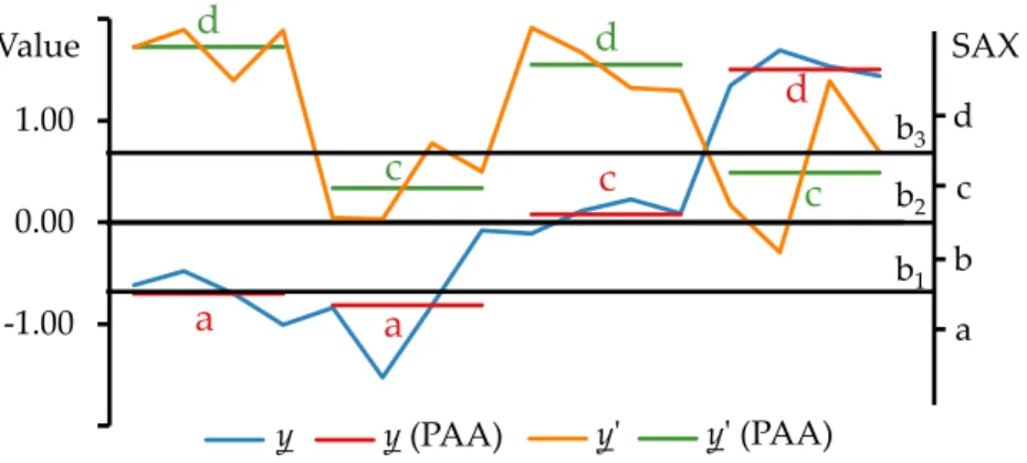
For example, Figure 3.2 shows a time seriesy (blue line, T = 4) from [SK08]. Its PAA representation (red segments,W = 4) isy¯| = (−0.70,−0.81,0.08,1.50). SAX visualizes
the symbols with alphabetic characters (“a", “b", . . . ) in order to stress their discrete nature. Given an alphabet A = 4 and respective breakpoints at 0.00 and±0.67 (black horizontal lines and x-axis), its SAX representation isyˆ|= (a, a, c, d).
The figure shows a second time seriesy0 (orange line) whose PAA and SAX representa-tions arey¯0| = (1.72,0.34,1.55,0.49)(green segments) andyˆ0| = (d, c, d, c), respectively. The Euclidean distance betweenyandy0is approx. 6.71, the PAA distance betweeny¯and
¯
y0is approx. 6.44, and the SAX distance betweenyˆandyˆ0is approx. 3.02. These distance measures have the following properties.
• The distance calculation only requiresW comparisons instead ofT comparisons. • PVQA and SAX use some storage to precalculate the distance. SAX stores the
distance between all symbols as a lookup table of size A2 so that d
SAX needs W
lookups. Thus, it does not call the cell function (Equation 3.12) and it avoids the comparisonsmin(a, a0)andmax(a, a0).
• The distance measures lower-bound the Euclidean distance,d∗(y, y0) ≤ dED(y, y0).
Thus, the Euclidean distance is considered the baseline distance between two time series that is calculated approximately and efficiently by shape-based distance mea-sures. For PVQA, the lower-bounding property has not been shown [MLW04]. By lower-bounding the Euclidean distance, shape-based distance measures fulfill an important requirement for time series matching.
Besides lock-step distance measures, techniques based on salient points apply relative distance measures [PWZP00, PF02] which relate the distance to the given values, and op-timization techniques [MW01]. Further discretization techniques apply string matching as distance measure [AJB97, HY99]. Other techniques do not require a distance measure for their application [QWW98, BYS08, Fu11].
3.3
MODEL-BASED ENGINEERING
While raw-data-based and shape-based engineering focuses on theeffectof a process ex-pressed by a time series or its comex-pressed shape, model-based engineering focuses on thecauseof the process expressed by a generativetime series model. This model consists of three components:
• The representation technique determines the class of the model which is assumed as cause of the time series.
• Metaparameters specify a model regarding important characteristics such as long-term or cyclically repeated characteristics.
• After identifying the representation technique and metaparameters,model parame-tersare estimated and form themodel-basedrepresentation of a specific time series.
Model-based engineering follows a life cycle with five stages (Figure 3.3).
1. Themodel identificationis the manual selection of a representation technique and of the manual or semi-automatic identification of metaparameters. Moreover, a dis-tance measure is selected that expresses the disdis-tance of two representations based on model parameters.
1. Model Identification 2. Model Estimation 3. Model Use 4. Model Evaluation 5. Model Maintenance
Figure 3.3: Life cycle of Time Series Model
2. The model parameters areestimatedsuch that they represent a time series accurately. 3. Subsequently, the model parameters are usedas model-based representation for a
data-mining task.
4. Model evaluationprovides diagnostic checks in order to re-evaluate the model. 5. Model maintenanceuses the results from diagnostic checks to improve model
identi-fication and estimation.
Subsequently, we give an overview of model-based representation techniques from the literature along with distance measures and discuss their properties.
3.3.1 Representation
There are five classes of model-based representation techniques that we assess subse-quently: statistical models, ARIMA models, Markov models, and artificial neural networks. Beyond, there are representation techniques such as Gaussian processes, time series bit-maps, or kernel models that have been applied rarely for more than one data-mining task which is why we do not include them in our assessment. More details on these techniques can be found in [MS82, Lia05, ASY15, BLB+17].
All these representation techniques are domain-independent since they focus on statisti-cal causes in a time series. Domain-dependent models such as models for atmospheristatisti-cal phenomena [KKD91, BdMK02], are out of scope because they take physical information into account which is why they cannot be applied to others domains.
Statistical Model
A statistical model gathers the statistical assumptions concerning the generation of a time series. It treats values of a time series as realizations of a random variableY and captures their distribution in a short representation. Formally, a statistical model is a pair(S,P)of the sample spaceSand a set of probability distributionsP. The sample space of a time se-ries is the space of real numbers. The probability distributions are usually parametrized, i.e.,P = {Pθ : θ ∈ Θ}where θis one set of model parameters from all possible sets of
model parametersΘ. It is assumed that there is a true probability distribution that gener-ates the time series values. The goal is to identify a set of probability distributionsP and estimate model parametersθsuch thatPθapproximates the true distribution [McC02].
For example, time series values are assumed to be normally distributed. The normal distribution N has two model parameters θ = (µ, σ2) where µ ∈ R is the mean and σ2 ∈R>0is the variance. Its probability density function is:
fY(y) = 1 √ 2πσ2exp(− (y−µ)2 2σ2 ) (3.13)
After the identification of normal distributions as underlying probability distributions
P, the model parameters have to be estimated to find Pθ ∈ P. This is carried out by a
maximum-likelihood estimation. The likelihood function for the time series valuesy1,
... ,yT is given by: L(µ, σ2;y1,..., yT) = YT t=1fY(yt;µ, σ 2) (3.14) = (2πσ2)−T/2· exp(− 1 2σ2 XT t=1(yt−µ) 2). (3.15) A logarithm is applied that leads to an easier calculation:
log(L(µ, σ2;y1,..., yT)) =− T 2 log(2π)− T 2 log(σ 2)− 1 2σ2 XT t=1(yt−µ) 2 (3.16)
Finally, if the log-likelihood is maximized, it provides the estimationsµˆandσˆ2 that ap-proximate the true distribution:
ˆ µ= 1 T XT t=1yt (3.17) ˆ σ2 = 1 T XT t=1(yt−µˆ) 2 =1 T XT t=1y 2 t −1 T XT t=1yt 2 (3.18) Overall, the normal distribution represents a time series with two real values that can be calculated in one pass. When it comes to generating time series for meteorology, other probability distributions, such as Weibull or Reighley distributions are also assumed [KKSM91]. Moreover, Gaussian mixture models which are combinations of normal dis-tributions have been applied to compute representations for audio signals [TW02].
ARIMA Model
The autoregressive integrated moving average (ARIMA) process provides a model for a variety of time series. It treats a time series as a realization from a stochastic process. As its name suggested, the model consists of an autoregressive (AR), a moving average (MA) part, and an integration (I) part that are derived from respective processes. Prerequisites of these processes are a white noise process and the linear process. First, we define these processes and second, we explain the parts of the ARIMA process.
White noise process An ARIMA process assumes that a time series is generated by a series of shocks which we call error terms at. These error terms are independentfrom
each other, randomlydrawn from a fixed distribution with mean 0 and variance σa2, or more succintlyat~iidN(0, σa2)where iid is a shorthand for independent and identically
distributed [SS11]. A series of these error terms ..., at−1, atis calledwhite noise process. If
the error terms areat~iidN(0,1), then the series is callednormalwhite noise process.
Linear process A process is calledstationaryif its probabilistic properties do not change over time and its values vary around a constant mean with a constant variance. Alinear processassumes that a time series is generated by a weighted sum of error terms:
˜
yt=at+ψ1at−1+ψ2at−2+ ... (3.19)
whereψ1,ψ2, ... are the weights andy˜t =yt−µˆis the time series corrected by its mean,
if it is stationary. To be a valid stationary process, it is necessary for the weights to be absolutely summable, i.e.,P∞
j=1|ψj|<∞. Under suitable conditions, the linear process can
also be regarded as weighted sum of past values ofy˜tplus an added error term:
˜
yt=
X∞
j=0πjy˜t−j+at (3.20)
In this form, the process can be regarded as “regressed” on itself: ytdepends on former
values plus noise.
Autoregressive process In practice, the representations of linear processes are not use-ful because they have an infinite amount of weights. Theautoregressive processassumes a stationary linear process. However, the current value of an autoregressive process of orderp, AR(p), is a finite, linear aggregate of previouspvalues:
˜
yt=φ1y˜t−1+φ2y˜t−2+... +φpy˜t−p+at (3.21)
whereφ1, φ2, ... , φp are the weights, andat is anerror termfrom a normal white noise
process.
Using the backshift operatorBwhich is defined asByt=yt−1and theoperatorof AR(p)
which is defined as:
φ(B) = 1−φ1B−φ2B2−...φpBp (3.22)
the autoregressive process may be written as:
φ(B)˜yt=at (3.23)
Moving average process Themoving average processis the second important stationary process. Instead on depending on former values of the process, a moving average process of the orderq, MA(q), assumes a finite, linear aggregateqof error terms that occurred at time instancetand before:
˜
yt=at−θ1at−1−θ2at−2− ... −θqat−q (3.24)
whereθ1,θ2, ... ,θqare weights. With the definition of an operator for MA(q):
θ(B) = 1−θ1B−θ2B2− ...θqBq (3.25)
the moving average process is written as:
˜
yt=θ(B)at (3.26)
Mixed autoregressive-moving average process For some time series, it is necessary to combine an autoregressive and moving average process to provide an accurate model. The ARMA(p, q) process combines an AR(p) and a MA(q) process as follows:
˜
yt=φ1y˜t−1+... +φpy˜t−p+at−θ1˜at−1− ... −φq˜at−q (3.27)
or