Optimisation
by
Thanh Dai Nguyen
BSc. (Honours)Submitted in fulfilment of the requirements for the degree of Doctor of Philosophy
Deakin University
October 2018
With the deepest appreciation, I would like to thank my executive supervisor A/Prof. Sunil Gupta for his guidance, encouragement and support throughout my research. With his deep insight, wisdom and patience, he has taught me invaluable knowledge and research skills. This thesis would have never taken shape without his thorough supervision.
I wish to thank my co-supervisor A/Prof. Santu Rana for providing constructive feedback and making suggestions on my papers and this thesis. I would never forget our valuable discussions.
It is my pleasure to acknowledge my associate supervisor Prof. Svetha Venkatesh for giving me the chance to do research at Deakin university. She has gave me valuable guidance, suggestions and advice in both research and life.
I would like to thank all staff and students of PRaDA for providing me a friendly working environments. I will always remember our full-of-laughter lunchtime dis-cussions.
Finally, this thesis is dedicated to my beloved family: my parents, my sisters, my brother and my wife who always support, encourage, and stand by my side when I needed them most.
Part of this thesis has been published or documented elsewhere. The details of these publications are as follows:
Chapter 3:
• Nguyen T.D., Gupta S., Rana S., Venkatesh S. (2017) Stable Bayesian Op-timization. In Advances in Knowledge Discovery and Data Mining (PAKDD 2017) (best student paper award).
• Nguyen T.D., Gupta S., Rana S., Venkatesh S. (2018) Stable Bayesian Op-timization. International Journal of Data Science and Analytics.
Chapter 4:
• Nguyen T.D., Gupta S., Rana S., Venkatesh S. (2016) Cascade Bayesian Optimization. In Advances in Artificial Intelligence (AI 2016).
• Nguyen T.D., Gupta S., Rana S., Venkatesh S. (2018) Bayesian Optimization for cascaded processes (under preparation to be submitted to Expert Systems with Applications).
Chapter 5:
• Nguyen T.D., Gupta S., Rana S., Venkatesh S. (2018) A Privacy Preserving Bayesian Optimization with High Efficiency. In Advances in Knowledge Dis-covery and Data Mining (PAKDD 2018) (best paper award).
Acknowledgements iv Relevant publications v Abstract xix Abbreviations xxi Notation xxii 1 Introduction 1
1.1 Aims and approaches . . . 3
1.2 Significance and contributions . . . 4
1.3 Structure of the thesis . . . 5
2 Related background 8
2.1 Experimental design . . . 8
2.2 Global optimisation . . . 9
2.3.1 Overview of Bayesian optimisation . . . 12
2.3.2 Applications of Bayesian optimisation . . . 13
2.4 Surrogate models . . . 18
2.4.1 Gaussian processes . . . 18
2.4.2 Random forests . . . 25
2.4.3 Deep neural networks . . . 26
2.5 Acquisition functions . . . 27
2.5.1 Improvement-based policies . . . 27
2.5.2 Optimistic policies . . . 31
2.5.3 Information-based policies . . . 31
2.6 Active research areas . . . 33
2.6.1 High-dimensional problems . . . 33
2.6.2 Constrained Bayesian optimisation . . . 34
2.6.3 Multi-objective Bayesian optimisation. . . 36
2.6.4 Transfer learning . . . 37
2.7 Open problems relevant to practical applications . . . 38
2.7.1 Stability . . . 38
2.7.2 Cascaded process optimisation . . . 39
2.8.1 Data perturbation methods . . . 40
2.8.2 Group anonymisation methods. . . 42
2.8.3 Methods for distributed data. . . 42
2.8.4 Differential privacy . . . 43
2.9 Summary . . . 45
3 Stable Bayesian optimisation 47 3.1 Introduction . . . 48
3.2 The proposed framework . . . 50
3.2.1 Stability of Gaussian process prediction . . . 50
3.2.2 Stable Bayesian optimisation. . . 53
3.3 Experiments . . . 59
3.3.1 Baseline method and evaluation measures . . . 60
3.3.2 Experiments with synthetic function . . . 60
3.3.3 Experiments with hyperparameter tuning problems . . . 62
3.4 Summary . . . 66
4 Bayesian optimisation for cascaded processes 67 4.1 Introduction . . . 68
4.3.1 Baseline method and evaluation measure . . . 79
4.3.2 Experiments with synthetic data . . . 79
4.3.2.1 Data generation . . . 79
4.3.2.2 Experimental results . . . 80
4.3.3 Experiments with tuning hyperparameters for data analytic pipelines . . . 82
4.3.3.1 Tuning hyperparameters for data analytic pipelines . 82 4.3.3.2 Experimental results . . . 82
4.3.4 Experiments with alloy heat treatment optimisation . . . 84
4.3.4.1 Alloy heat treatment . . . 84
4.3.4.2 Experimental results . . . 85
4.3.5 Cost-efficient optimisation . . . 86
4.4 Summary . . . 86
5 A new privacy framework for Bayesian optimisation and other al-gorithms 88 5.1 Introduction . . . 89
5.2 The new privacy framework . . . 92
5.3 Privacy preserving Bayesian optimisation . . . 93
5.4 Application of EPP framework for other machine learning algorithms 105
5.4.1 EPP based K-means clustering . . . 105
5.4.2 Experiments . . . 109 5.5 Summary . . . 117 6 Conclusion 118 6.1 Summary . . . 118 6.2 Future directions . . . 120 Bibliography 122
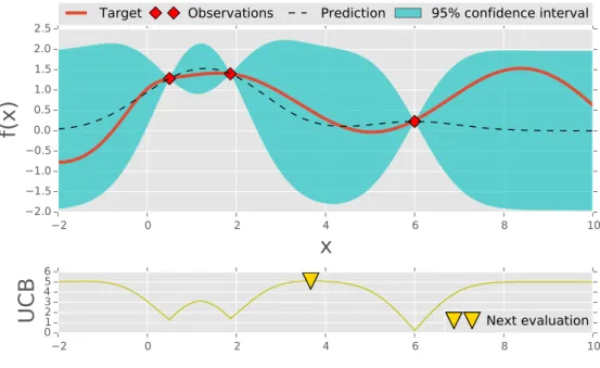
2.1 Visualisation of the surrogate model and the acquisition function of Bayesian optimisation. In this illustration, a Gaussian process and its upper confidence bound (UCB) are used for the surrogate model and the acquisition function. The graph in red colour shows the true objective function. The dotted line represents the mean of Gaussian process posterior. The blue area indicates 95% confidence interval. The yellow triangle represents maximum value of the acquisition func-tion, suggesting the next point for evaluation. . . 14
2.1 Visualisation of the surrogate model and the acquisition function of Bayesian optimisation. In this illustration, a Gaussian process and its upper confidence bound (UCB) are used for the surrogate model and the acquisition function. The graph in red colour shows the true objective function. The dotted line represents the mean of Gaussian process posterior. The blue area indicates 95% confidence interval. The yellow triangle represents maximum value of the acquisition func-tion, suggesting the next point for evaluation. . . 15
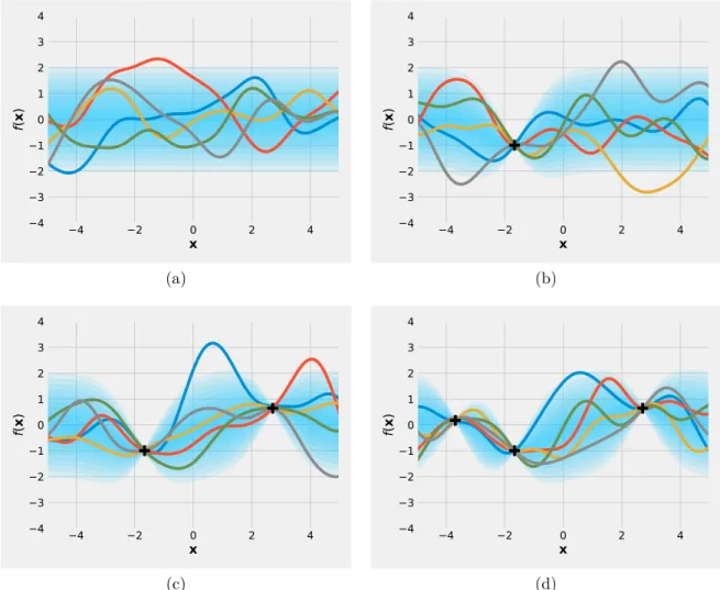
2.2 An example of Gaussian process for a one dimensional function. Dif-ferent shades of blue represent the predictive density at each input location. The colour lines illustrate some samples drawn from Gaus-sian posterior distribution. Fig. 2.2a shows a GausGaus-sian process prior and its samples. The remaining plots show Gaussian process posteri-ors after observing few samples from a function. . . 19
smoother. . . 24
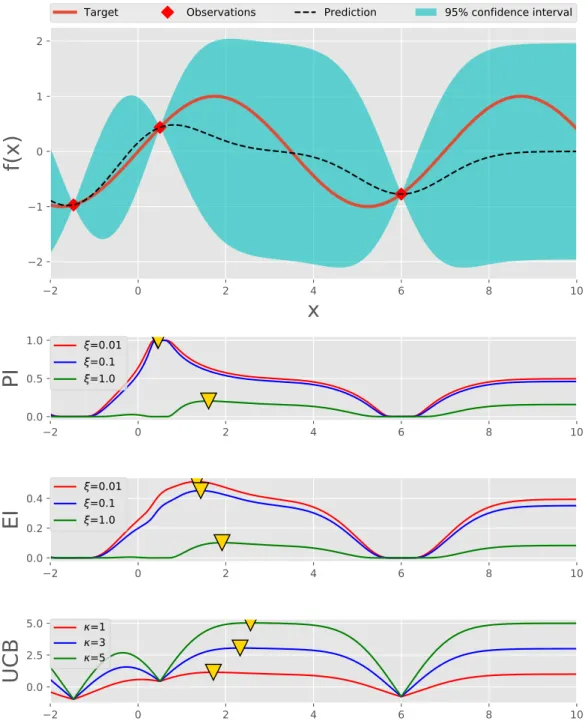
2.4 Examples of acquisition functions. The top plot is the Gaussian model with 3 observations. The remaining plots are the acquisition func-tions for the Gaussian process: PI - Probability Improvement (see Eq. (2.17)), EI - Expected Improvement (see Eq. (2.19)), UCB - Up-per Confidence Bound (see Eq. (2.21)). The yellow triangle makers are the maximum of the acquisition functions. . . 28
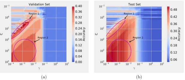
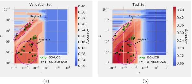
3.1 Performance versus hyperparameters for a Support Vector Machine training as colour coded images: a) on a small validation set, and b) on a large test set. Spurious peaks of region 1 seen for the validation set vanish for the test set while the stable peak of region 2 still remains. 49
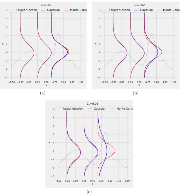
3.2 Predictive distributions of Gaussian approximation and Monte-Carlo approximation with respect to different values of noise levels: a)Σx =
0.01, b)Σx = 0.02, c)Σx= 0.05. In practice, parameter settings are
limited to 1% perturbation and our approximation based on Gaussian distribution can handle it well.. . . 54
3.3 a) The synthetic function with one stable peak and multiple spuri-ous peaks b) The STABLE-UCB acquisition function and aleatoric variance after 30 iterations. . . 61
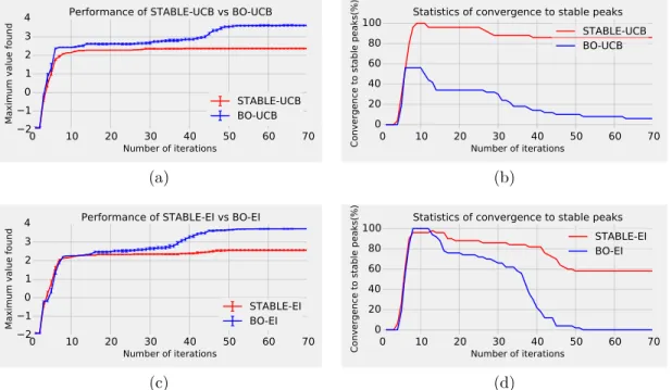
3.4 Performance of stable Bayesian optimisation and standard Bayesian optimisation with respect to number of iterations on Synthetic func-tion. a) and c) shows that STABLE-UCB and STABLE-EI converge to 2.3 and 2.5 (stable peak) whereas BO-UCB and BO-EI converge to 3.7 (spurious peak). b) and d) shows that stable Bayesian optim-isation reaches stable peak more often than the baseline. . . 61
dataset and b) on test dataset. The background portrays the per-formance function with respect to the hyperparameters. Spurious peaks (region 1) is evident for the validation dataset but vanished for the test set while stable region (region 2) still remains. . . 63
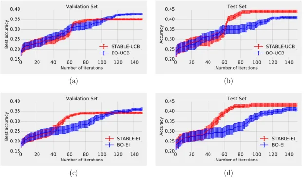
3.6 Performance of stable Bayesian optimisation and standard Bayesian optimisation using SVM with respect to number of iterations on Let-ter dataset. The performance of standard Bayesian optimisation, due to convergence to spurious peaks on the validation set (Fig 3.6a and Fig 3.6c), results in poor performance for the test set (Fig 3.6b and Fig 3.6d). . . 64
3.7 Performance of stable Bayesian optimisation and standard Bayesian optimisation using SVM with respect to number of iterations on Glass dataset. The performance of standard Bayesian optimisation, due to convergence to spurious peaks on the validation set (Fig 3.7a and Fig 3.7c), results in poor performance for the test set (Fig 3.7b and Fig 3.7d).. . . 65
4.1 A diagram of a multi-stage cascaded process. Input (e.g. raw ma-terial) is transformed under the conditions set by control parameters. The output of each stage then becomes the input for the next stage. The output of the last stage is often the quantity that we are inter-ested in optimising as a function of the controls. . . 68
4.2 Notations of input, output and control parameters of a cascaded pro-cess. For each stages,us
t,vst andwst are the input, control parameters
and output at iterationt; andGPstis the Gaussian process model built at iteration t. . . 71
the left column, number of control parameters per stage is fixed at 4 but the number of stages are varied. In the right column, number of stages is fixed at 5, but the number of control parameters per stage is varied. . . 81
4.4 Performance of cascade Bayesian optimisation and joint Bayesian op-timisation using SVM with respect to number of iterations on tuning hyperparameters of a data analytic pipeline (a) Letter dataset (b) Glass dataset. . . 83
4.5 Best hardness achieved as a function of number of iterations for both cascade BO (red) and joint Bayesian optimisation (blue), for different cost parameter λ . . . 85
4.6 Experimental result for Aluminium Scandium hardening: Hardness of alloy (red) and time (blue) vs cost parameter λ . . . 86
5.1 Privacy preserving Bayesian optimisation framework. The optimisa-tion process is a three-step procedure. The first step is to evaluate the objective function at the input suggested by optimiser. The second step is to perturb the output by a noise to ensure the privacy. The third step is at the untrusted end where optimiser is used to suggest the next point for evaluation. . . 91
5.2 Using Error Preserving Privacy framework for machine learning al-gorithms. . . 94
5.3 The ratio En+1
En versus qn+1. We set qn+1 =α so that
En+1
En ≥exp(−). 98
5.4 Best value so far with respect to Bayesian optimisation iteration. The reported values are noise-free values of the function a) Branin 2D, b) Rosenbrock 4D, c) Hartmann 4D, d) Hartmann 6D. . . 101
with different level of privacy: a)= 0.1 (high privacy) and b)= 0.5 (low privacy). The blue and the magenta show the best function value achieved so far from the experimenter’s perspective and optimiser’s perspective, respectively. . . 102
5.6 Optimisation results for two real datasets. . . 104
5.7 Results using Synthetic dataset with N = 180, K = 3. (a) Average perturbation in cluster centroid with respect to , (b) NMI with re-spect to , (c) Ratio of variance for estimation errors Einc and Eexc,
(d) NMI for varying number of data points at = 0.1.. . . 112
5.8 Results using Seeds dataset with n = 210, K = 3, (a) Average per-turbation in cluster centroid with respect to , (b) NMI with respect to, (c) Ratio of variance for estimation errorsEinc andEexc, (d) NMI
for varying number of data points at = 0.1. . . 114
5.9 Results using UKM dataset with n = 258, K = 4, (a) Average per-turbation in cluster centroid with respect to , (b) NMI with respect to, (c) Ratio of variance for estimation errorsEinc andEexc, (d) NMI
5.1 Comparison with the baselines in terms of various metrics at= 0.1. Average results over 30 random centroid initialisations are reported with the standard errors in parenthesis. The bold face indicates the best results among private algorithms. . . 116
2.1 Bayesian optimisation algorithm . . . 12
3.1 The proposed stable Bayesian optimisation. . . 53
4.1 Cascade Bayesian optimisation algorithm . . . 73
5.1 Error Preserving Private Bayesian Optimisation (EPP-BO) . . . 99
5.2 Error Preserving Private K-means algorithm . . . 109
Bayesian optimisation is a powerful machine learning method that allows efficient optimisation of expensive black-box functions. Recently, Bayesian optimisation has been applied successfully in several applications like robotic, material design and automated machine learning. However, despite its recent advancement, applying Bayesian optimisation in practical settings still faces many challenges. This thesis focuses on addressing these practical challenges. The contributions of this thesis are new Bayesian optimisation algorithms for three practical problems: i) finding stable optimum of functions that may have several narrow peaks/valleys, ii) optim-ising multi-stage cascaded structure processes, and iii) developing a privacy-aware algorithm when it is not possible to reveal the optimum for untrusted optimisers.
In many real world systems, the optimisation surface contains multiple peaks/valleys with different widths. For such applications, if the optimisation has converged to a narrow peak/valley, the utility of the solution will be seriously limited due to the imprecise nature of the systems. We address this problem through a novel stable Bayesian optimisation framework. We construct two new acquisition functions that help Bayesian optimisation to avoid the convergence to narrow (sharp) peaks. We theoretically analyse our algorithm and guarantee that Bayesian optimisation using the proposed acquisition function favours stable (wide) peaks over the unstable (narrow) ones. We demonstrate the effectiveness of our proposed algorithm on both synthetic function optimisation and hyperparameter tuning for support vector machines.
Multi-stage cascaded structure processes are fairly common in manufacturing in-dustry. In a cascaded process, the input of each stage is transformed under
parameters correctly. We propose a novel cascade Bayesian optimisation algorithm that effectively optimises cascaded structure processes. At the last stage, we use the standard Bayesian optimisation to find the input and control parameters that maximise its output quality. For the remaining stages, we formulate a novel optim-isation problem. In a back-propagation manner, we solve this problem to find the input and control parameters of the remaining stages through the inversion of the Gaussian processes. We incorporate a cost-sensitive component to the formulation to discover cost-efficient solutions. We theoretically analyse and show the conver-gence rate our proposed algorithm. Experiments with a heat treatment testbed of an Al-Sc alloy and hyperparameter tuning of data analytic pipelines show the efficacy of our algorithm.
In industry, experimenters, who are domain experts of their fields, may not have mathematical optimisation expertise. To find the optimal design, they may require third-party optimisation services. Since the optimal design is the key to a business’s success, it often can not be disclosed to the third-party optimisers. To address the privacy concerns, we firstly propose a novel privacy preserving framework called Er-ror Preserving Privacy (EPP) that provides strong privacy guarantee while ensuring high utility. Using EPP framework, we propose a privacy preserving Bayesian op-timisation that helps the experimenters to find the optimal design without revealing it to the untrusted optimisers. We theoretically analyse the algorithm and derive the bound on the amount of noise required to guarantee the privacy. We demonstrate the applicability of our EPP framework by constructing a novel privacy preserving K-means clustering algorithm. Using both synthetic and real datasets, we show that the efficiency of our proposed Bayesian optimisation and K-means clustering algorithms is comparable to non-private algorithms and significantly better than the baseline.
BO Bayesian Optimisation
DNGO Deep Networks for Global Optimisation DP Differential Privacy
EI Expected Improvement EPP Error Preserving Privacy
GP Gaussian Process
GP-UCB Gaussian Process - Upper Confidence Bound PESC Predictive Entropy Search with Constraints
PI Probability of Improvement PINQ Privacy Integrated Queries
RBF Radial Basis Function
REMBO Random Embedding Bayesian Optimisation SMAC Sequential Model-based Algorithm Configuration SMBO Sequential Model-based Bayesian Optimisation
SVM Support Vector Machine UCB Upper Confidence Bound
R the set of real numbers
x vector x
x scalar x
D dataset
diag(w) a diagonal matrix containing the elements of vector w
E expectation
Var variance
GP Gaussian process
K covariance matrix
k(x,x0) covariance function evaluated at xand x0
N normal distribution
Φ(.) the standard normal cumulative distribution function
φ(.) the standard normal probability density function
α(x;Dt) acquisition function at xgiven a dataset Dt X search space
O(.) big O notation
p(y|x) probability density of conditional random variable y given x P probability
kT the transpose of vector k
∼ distributed according to; example x∼ N(0,1)
µ(.) Gaussian process posterior mean
σ2(.) Gaussian process posterior variance
H(X) entropy of random variable X
Lap Laplace distribution
x1:t set oft vectors from x1 to xt
y1:t set oft scalars from y1 to yt
Introduction
Experimental designs are crucial in research and development: scientists design experiments to discover and understand physical or social phenomena, widening the horizon of human knowledge; material researchers design new type of alloys that are strong and light; meteorologists design sensor networks to monitor the environment; pharmaceutical researchers design new type of drugs to fight diseases. In all of these applications, the objective is to find the optimal design to achieve the “best” possible outcome. The relation between the output and design variables can often be represented through a mathematical function. However, this function may not be expressed in a closed form and its evaluation is generally expensive. This make the task of finding the optimal design a nontrivial problem.
Bayesian optimisation has emerged as a powerful method for finding such optimal designs. It has seen successful applications in robotics (Lizotte et al.,2007;Calandra et al., 2014b; Martinez-Cantin et al., 2009), environmental monitoring (Srinivas et al., 2010), automated machine learning (Thornton et al., 2013; Hoffman et al.,
2014), material design (Li et al.,2017), sensor networks (Garnett et al.,2010;Srinivas et al.,2010), reinforcement learning (Brochu et al.,2010b), combinatorial optimisa-tion (Hutter et al.,2011; Wang et al., 2013) and interactive user-interfaces (Brochu et al., 2010a). Due to popularity of Bayesian optimisation in so many applications, there have been efforts to extend its reach to more complex but useful problems such as optimisation in high dimensional spaces (Chen et al., 2012; Wang et al., 2013), and adding the ability to transfer source (function) knowledge to target functions
(Joy et al., 2016b; Shilton et al., 2017), multi-objective optimisation (Feliot et al.,
2017), parallel optimisation (Azimi et al., 2010; Nguyen et al.,2016), etc.
In spite of recent progress, Bayesian optimisation methods still face several chal-lenges in practice. In many real-world systems, the objective function contains multiple peaks with different widths. For such applications, the utility of the op-timal design (solution) can be seriously limited if the optimisation has converged to a narrow peak. This is because of the imprecise nature of such systems. For example, in an alloy design process, a goal may be to find a mixing proportion of a set of elements that yields the highest value of strength. However, it is practically nearly impossible to mix the elements in exact proportion due to the impurities in raw materials. Thus, if the optimal proportion is at a narrow peak of the surface then the strength of the alloy may dramatically reduce depending on values of im-purities. Therefore, there is a need for a stable Bayesian optimisation framework that is able to find stable solutions.
Another important situation is where design optimisation is highly desired in in-dustrial processes. Inin-dustrial processes often have multi-stage cascaded structure. A cascaded structure process consists of several stages, each stage’s input is the output from the previous stage. The standard Bayesian optimisation approach con-siders the whole cascaded process as one single black-box function and does not take into account the cascaded structure. Thus the problem becomes optimising a high-dimensional target function, which is a difficult task. Therefore, there is a need for a Bayesian optimisation algorithm that can utilise the cascaded structure in the optimisation.
Yet another important challenge in using Bayesian optimisation for real-world ap-plications is privacy. In industry, experimenters, who are domain experts of their specific fields, may not have the mathematical optimisation expertise and thus re-quire third-party optimisation services to find the optimal design. Since the optimal design is the key to a business’s success, it often can not be disclosed to the third-party optimisers. One approach to address this problem is to use privacy preserving approaches for Bayesian optimisation. It is important to have a Bayesian optimisa-tion algorithm that helps the experimenters to find the optimum of the objective function without disclosing the exact details of the optimal design while ensuring a minimum compromise on the optimality or the quality of the design.
1.1
Aims and approaches
The goal of this thesis is to expand the knowledge base by addressing several chal-lenges in applying Bayesian optimisation for real-world applications. In particular, we aim to develop Bayesian optimisation algorithms that are able to achieve the following objectives:
1. Finding stable solutions (wide peaks) for optimisation problems instead of unstable solutions (narrow peaks) where possible.
2. Optimising processes that have multi-stage cascaded structure.
3. Developing a privacy-aware Bayesian optimisation technique when it is not possible to reveal the exact value of the optimal solution to third-party un-trusted optimisers.
To achieve these aims, we leverage recent advances in machine learning, especially in Bayesian optimisation and Gaussian processes to implement the following ap-proaches:
• To realise Aim 1,i.e. to find stable solutions in optimisation, we use a modified Gaussian process model that takes into account any perturbations in the input variables. The extra variance due to the perturbations is included in the formulation of two novel acquisition functions for Bayesian optimisation. We theoretically analyse the two new acquisition functions and prove that they are guaranteed to have higher values for “more stable” peaks. Thus the Bayesian optimisation algorithm using these acquisition functions have higher tendency to sample in the area around the stable peaks.
• To realise Aim 2, i.e. to take advantage of multi-stage cascaded structures, each stage of a cascaded process is modelled by an independent function through separate Gaussian processes. Using the Gaussian process of the final stage, we use the standard Bayesian optimisation to find the input and control parameters of the final stage that maximise its output quality. For the remain-ing stages, in a back-propagation manner, we formulate a novel optimisation
problem. We solve this problem to find the input and control parameters of the remaining stages through the inversion of the Gaussian process. We introduce costs associated with the control parameters in the optimisation formulation to discover cost-efficient solutions.
• To realise Aim 3,i.e. to address the privacy concerns in using Bayesian optim-isation, we firstly propose a novel privacy preserving framework called Error Preserving Privacy (EPP) that provides strong privacy guarantee while en-suring high utility. Using EPP framework, we propose a privacy preserving Bayesian optimisation that helps an experimenter in an industry to find the optimum of an expensive black-box function without revealing the exact func-tion values. The EPP framework helps to maintain high optimisafunc-tion efficiency even under stringent privacy requirements. Under certain assumptions on the adversary’s model, we theoretically analyse the algorithm and derive the bound on the amount of noise required to guarantee the privacy. To demonstrate the applicability of EPP framework, we construct a novel privacy preserving K-means clustering algorithm.
1.2
Significance and contributions
This thesis is significant because: (i) it develops novel algorithms to address several practical challenges of Bayesian optimisation and (ii) it applies these algorithms to a wide range of practical problems in machine learning and industrial processes. In particular, our main contributions are:
• We provide a definition for stability of a peak. Based on our definition of stabil-ity, it is possible to measure the stability of a peak using a modified Gaussian process model with input perturbation. We propose two novel acquisition functions for Bayesian optimisation that actively seek the stable peaks of the objective function. We theoretically prove that under mild assumptions, when two peaks are of the same height, the proposed acquisition functions would always favour the more stable peak. We validate the effectiveness of our pro-posed method using both synthetic and real datasets.
• A cascade Bayesian optimisation framework that effectively optimises multi-stage cascaded processes. We formulate a novel optimisation problem to find the desired input quality and control parameters at intermediate stages of a cascaded process. We theoretically analyse the proposed solution and show that the convergence rate of our algorithm is sub-linear in the number of evaluations. We demonstrate the efficacy of our algorithm on synthetic data, tuning data analytic pipelines and alloy heat treatment optimisation.
• A new privacy preserving framework that provides strong privacy guarantees while ensuring high utility. We propose a novel privacy preserving Bayesian optimisation algorithm under the proposed privacy framework that helps ex-perimenters in an industry to utilise the expertise of a third-party optimisation service without revealing the exact function values. We theoretically analyse the proposed algorithm and derive bounds on the amount of noise required to ensure the privacy. We validate the effectiveness of our method on both synthetic and real dataset. In addition, we demonstrate the applicability of our proposed privacy preserving framework by developing a novel privacy pre-serving K-means algorithm with high utility. We illustrate and validate the efficacy of the proposed K-means algorithm through experiments with both synthetic and real datasets.
1.3
Structure of the thesis
The remainder of this thesis is organised as follows:
• Chapter 2 provides the preliminary background and research works relevant to the problems considered in this thesis. We first briefly discuss about experi-mental design and the importance of optimal design problem. We then review several popular global optimisation methods. The chapter then focuses on Bayesian optimisation method and its applications, followed by a discussion about various choices for surrogate models and acquisition functions. In the subsequent part of chapter 2, we review active research areas of Bayesian op-timisation, and then discuss about several open problems that are relevant to
practical applications. The chapter ends by reviewing the literature in privacy preserving machine learning methods.
• Chapter3 begins with the presentation of our first contribution of developing a stable Bayesian optimisation framework. We define the notion of stabil-ity and introduce a modified Gaussian process model for noisy inputs. The variance in the modified Gaussian process posterior distribution consists of epistemic and aleatoric components, among which the aleatoric variance is the one that affects the stability of the solutions. By incorporating the aleatoric variance information, we next propose two novel acquisition functions that help Bayesian optimisation to avoid the convergences to the sharp peaks. The chapter then provides theoretical analysis of the algorithm and guarantees that the proposed stable Bayesian optimisation algorithm prefers the stable peaks over unstable ones. Finally, the experimental results with both synthetic function optimisation and hyperparameter tuning show the effectiveness of our proposed method.
• Chapter 4proposes a novel framework, called cascade Bayesian optimisation, that deals with the optimisation of multi-stage cascaded processes. The pro-posed cascade Bayesian optimisation algorithm extends the standard approach by considering the objective as a series of optimisation problems that are solved sequentially from the last stage to the first stage. The cost is also incorporated into the formulation for cost-sensitive problems. We then theoretically analyse the cascade Bayesian optimisation algorithm and show the convergence rate of the proposed method. Finally, experiments using a simulated testbed of Al-Sc heat treatment and a data analytic pipeline are conducted to validate the efficiency of our proposed algorithm.
• Chapter 5 addresses the privacy concerns in applying Bayesian optimisation for practical applications. We first propose a novel privacy preserving frame-work, called Error Preserving Privacy (EPP), that stops an adversary from inferring sensitive information. By focusing directly on the estimation errors, EPP is able to provide privacy guarantees while the perturbation required is lower compared to traditional privacy preserving approaches. Under EPP framework, we present a novel Bayesian optimisation algorithm that can al-low experimenters from an industry to utilise the expertise from a third-party optimisation service in a privacy preserving manner. We next demonstrate
the effectiveness of our privacy preserving Bayesian optimisation algorithm on both benchmark functions and optimisation problems from real-world pro-cesses. In the remainder of this chapter, we demonstrate the applicability of EPP framework for other machine learning algorithms by presenting a new privacy preserving K-means clustering algorithm. By conducting experiments on both synthetic and real world datasets, we show that the efficiency of the proposed privacy preserving K-means algorithm is comparable to non-private algorithms and significantly better than the baseline.
• Chapter 6 summarises the main content of the thesis, and discusses about potential future research directions.
Related background
In this chapter, we present preliminary background and discussion of related works to this thesis. This chapter starts with the discussion of experimental design and its importance in scientific research. We then present a brief literature review of global optimisation and popular global optimisation approaches. The next part of this chapter focuses on Bayesian optimisation literature and its applications, followed by the discussion about various choices for the surrogate model and acquisition func-tion of Bayesian optimisafunc-tion. We then review active research areas of Bayesian optimisation and discuss about open problems that are relevant to practical applic-ations. We end this chapter by reviewing literature of privacy preserving in machine learning, which is one of the problems we aim to tackle in this thesis.
2.1
Experimental design
An experiment is a test or a series of tests that is designed to discover something about a particular process or system. In experiments, changes are purposely made to the input variables so that we may identify the reason for the changes observed in the output responses (Montgomery, 2017). This is different from observational study in which the main task is to observe and collect data without making any changes to the input.
Experiments play vital roles in science and engineering. They appear in many aspects of engineering such as new product design, manufacturing process, process improvement, etc. In many cases, the objective is to plan, conduct the experiments and analyse the observed data such that the useful conclusions are drawn.
Optimised experimental designs can result in immediate products improvement and innovation for a wide range of areas. For example, in material design, suppose a material engineer is interested in designing a new type of alloy. Here the objective is to determine the type and amount of materials to use to produce the highest hardness. The experimenter has to melt and mix different sets of elements and measure the hardness of the specimen. From the results of several such experiments, the engineer selects the combination that produces the highest hardness. Optimised experimental designs will help the material engineer to understand the process better and achieve desired results. Thus, design of experiments is crucial in science and technology.
In the design of experiments, finding the best design efficiently is important since it helps to reduce the cost of experimentation. One approach to find the best design is to model the objective (e.g. hardness) as a function of input variables (e.g. proportion of materials). Then optimisation techniques can be used to find the optima of the objective function. The objective functions are typically non-convex having several peaks or valleys. Finding optima of such functions requires global optimisation and is a non-trivial task. In the following section, we will review the global optimisation problem and popular global optimisation approaches.
2.2
Global optimisation
The problem of finding global optimum of a function can be written as follows:
max
x∈X f(x) (2.1)
where f is the objective function andX is the domain. The target functionf could be as simple as speed of a car, or as complicated as the tastiness of cookies. The domain X could be amount of burning gasoline, or the proportion of ingredients of
the cookies.
There has been a lot of research for global optimisation in these situations. In the following, we will review some global optimisation approaches that may be relevant to this thesis.
Lipschitz methods Lipschitz methods are based on the assumption that the objective function is Lipschitz-continuous, meaning there exists a constant L ≥ 0 for which
|f(x1)−f(x2)| ≤Lkx1−x2k,∀x1,x2 ∈ X. (2.2)
When more and more function values are observed, this assumption effectively gives a lower and upper bound on the function. One can use these bounds to define the next observations to be acquired. There have been many variations of Lipschitz methods (Shubert,1972;Jones et al.,1993), but one common approach is to evaluate the objective function f where its upper bound is highest. After getting this new observation, the upper bound is updated and maximised to find the next point to evaluate.
Simulated annealing methods These methods are based on the physical ana-logy of cooling crystal structures. In this approach, at iteration t, the function is evaluated at the next trial point xt+1, and the assignment of the “current point”
xcurr depends on theacceptance distribution:
P(xt+1 →xcurr) = min ( 1,exp " f(xt+1)−f(xcurr) τt #) (2.3)
where τ is the “temperature” parameter. From (2.3), we can see that if f(xt+1)≤
f(xcurr), we will assign the newly proposed point xt+1 to the current point xcurr
with some probability, and we will always move to the new point otherwise. The sequence {τt} is referred as cooling schedule, and decreases toward 0, making the
algorithm escapes from local optima (Horst and Pardalos,2013). This method can be applied for combinatorial optimisation problems (Kirkpatrick et al., 1983), or continuous problems (Bélisle et al.,1993).
Genetic algorithms The term “genetic algorithms” is often referred to the class of algorithms that resembles the natural selection and reproduction processes. In these approaches, a candidate solution can be considered as an individual in a pop-ulation. Each individuals can evolve over time depending on its adaptiveness to the environment. Candidate solutions are perturbed according to biologically-inspired rules, resulting new candidates. The poorly performed candidates are removed from the population. This process is repeated until no further improvement is made. Some examples of genetic algorithms can be seen in (Holland, 1992; Bethke, 1978;
Liepins and Hilliard, 1989).
Multi-start local optimisation When function form is known and its derivat-ives exist, local optimisation methods can work really well, and a natural approach is to use them for global optimisation. The simplest adaptation of local optimisa-tion methods is using random restarts: one can uniformly draw points from search domain X, and have a local optimiser started from each point. As the number of starting points approaches infinity, all local maxima may have been found, thus we can simply select the best one we have observed.
2.3
Bayesian optimisation
Thus far, we have reviewed several global optimisation approaches. These ap-proaches work well for optimisation of functions that have either known mathem-atical forms or cheap to evaluate. However, in the case the objective functions are
unknown black-box functions and expensive to evaluate, standard global optimisation approaches often have poor performance. In this section, we review Bayesian optim-isation - an efficient global optimoptim-isation technique for expensive black-box functions. We will start by providing an overview of Bayesian optimisation, followed by a dis-cussion of successful applications of Bayesian optimisation.
2.3.1
Overview of Bayesian optimisation
Bayesian optimisation (Kushner, 1964; Mockus et al., 1978; Mockus, 1994) is a well-known methodology to find the optimum of an unknown expensive black-box function f. This optimisation problem can be formally defined as:
x∗ = argmaxx∈Xf(x) (2.4)
where X is the domain ofx. In global optimisation, X is often a compact subset of
Rd but Bayesian optimisation can be applied for more unusual search spaces such as
combinatorial search spaces. It is assumed that although f is a black-box function without a closed-form expression, it can be evaluated at any point xin the domain. This evaluation produces the outputy=f(x) +, whereis the measurement noise. Although this is the minimum requirement for Bayesian optimisation framework, gradient information, if available, can be incorporated to the algorithm as well.
Algorithm 2.1 Bayesian optimisation algorithm
1: Input:
2: Initial observation set Dt0 ={x1:t0, y1:t0}.
3: Bounds for the search space X.
4: Output: {xt, yt}Tt=1
5: for t=t0, . . . , T −1
6: Construct a surrogate model and an acquisition functionα(x;Dt) (see
Sec-tion 2.5 for details).
7: Select xt+1 by maximising acquisition functionα
xt+1 = arg max
x∈X α(x;Dt)
8: Evaluate the target function to obtain yt+1.
9: Augment the observation set: Dt=Dt∪ {xt+1, yt+1}.
10: Update the surrogate model.
11: end for
Bayesian optimisation is a sequential search algorithm. Given a few input and output observations of the function f, Bayesian optimisation iteratively suggests the next sample for evaluation to find the optimum value of the function. In other words, at iteration t, Bayesian optimisation selects a location xt+1 at which to
query f and get the observation. After a predefined number of queries T (defined by evaluation budget), the algorithm stops and returns its best estimates of the
function’s optimum.
Bayesian optimisation framework consists of two key components. The first is a (probability) surrogate model that can be evaluated at any point. This surrogate model uses prior knowledge, such as smoothness, about the cost function and known datapoints to capture and update our beliefs about the function. There are plenty of choices for this function such as Gaussian process (Rasmussen and Williams,2006), neural networks (Snoek et al.,2015), random forest (Brochu et al.,2010b), etc. The
second component of a Bayesian optimisation algorithm is an acquisition function that suggests where to evaluate the function next. After observing the output of each function evaluation, the algorithm updates the prior and produces a more inform-ative posterior distribution over objective functions. Using the acquisition function, the original problem becomes optimising a less expensive non-convex function. The acquisition function maintains a trade-off between exploration (where the surrogate model has high uncertainty about the function value) and exploitation (where the surrogate model has high predictive value). This technique is able to minimise the number of the function evaluations. The details of Bayesian optimisation algorithm are provided in Algorithm 2.1.
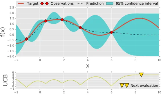
Fig. 2.1 is the illustration of using Bayesian optimisation for optimising a 1-D function. The surrogate model is the Gaussian process and the acquisition function is upper confidence bound (UCB, see (2.21)). As we can see from the figures, after 3 steps, there are 3 regions with high uncertainties including the region with global optimum. Bayesian optimisation continuously suggests points for evaluation and after 6 iterations, the global optimum is found.
2.3.2
Applications of Bayesian optimisation
Before going into details of two main components of Bayesian optimisation, we present an overview of various applications of Bayesian optimisation.
2 0 2 4 6 8 10
x
2.01.5 1.00.5 0.0 0.5 1.01.5 2.0 2.5f(x)
Target
Observations
Prediction
95% confidence interval
2 0 2 4 6 8 10
01 23
456
UCB
Next evaluation
(a) Surrogate model and acquisition function after 3 steps
2 0 2 4 6 8 10
x
2.01.5 1.00.5 0.0 0.5 1.01.5 2.0 2.5f(x)
Target
Observations
Prediction
95% confidence interval
2 0 2 4 6 8 10
01 23
456
UCB
Next evaluation
(b) Surrogate model and acquisition function after 4 steps
Figure 2.1: Visualisation of the surrogate model and the acquisition function of Bayesian optimisation. In this illustration, a Gaussian process and its upper confid-ence bound (UCB) are used for the surrogate model and the acquisition function. The graph in red colour shows the true objective function. The dotted line repres-ents the mean of Gaussian process posterior. The blue area indicates 95% confidence interval. The yellow triangle represents maximum value of the acquisition function, suggesting the next point for evaluation.
2 0 2 4 6 8 10
x
2.01.5 1.00.5 0.0 0.5 1.01.5 2.0 2.5f(x)
Target
Observations
Prediction
95% confidence interval
2 0 2 4 6 8 10
10 12 34 56
UCB
Next evaluation
(c) Surrogate model and acquisition function after 5 steps
2 0 2 4 6 8 10
x
2.01.5 1.00.5 0.0 0.5 1.01.5 2.0 2.5f(x)
Target
Observations
Prediction
95% confidence interval
2 0 2 4 6 8 10
10 12 34 56
UCB
Next evaluation
(d) Surrogate model and acquisition function after 6 steps
Figure 2.1: Visualisation of the surrogate model and the acquisition function of Bayesian optimisation. In this illustration, a Gaussian process and its upper confid-ence bound (UCB) are used for the surrogate model and the acquisition function. The graph in red colour shows the true objective function. The dotted line repres-ents the mean of Gaussian process posterior. The blue area indicates 95% confidence interval. The yellow triangle represents maximum value of the acquisition function, suggesting the next point for evaluation.
Robotics and reinforcement learning
Gait optimisation is a fundamental and challenging problem in robotics research. The tuning of gait parameters is time-consuming even for a simple robot. InLizotte et al. (2007), the authors proposed a new approach to gait learning based on Gaus-sian process optimisation. By parameterising the robot’s gait, the optimisation for gait velocity and gait smoothness was done on the Sony AIBO ERS-7 robot (Lizotte et al., 2007). In another work, different gait optimisation methods were compared and the Bayesian optimisation approach was shown to perform considerably better than grid or random search (Calandra et al., 2014b). Similarly, Bayesian optim-isation was successfully applied for mobile robot to find the optimal sensing path (Martinez-Cantin et al., 2009).
An example of using Bayesian optimisation for reinforcement learning was presen-ted in Brochu et al. (2010b), where Bayesian optimisation was used in tuning the parameters of a neural network policy and learning value functions at higher levels of the hierarchy. In another work, Wilson et al. (2014) proposed an effective ap-proach for applying Bayesian optimisation to reinforcement learning by exploiting the sequential trajectory information generated by reinforcement learning agents.
Environmental monitoring and sensor networks
In environmental monitoring, sensors networks are used to monitor quantities such as temperature, pollution level in soil, oceans, etc. Using sensor networks, we might find locations that have the highest temperature in a building by activating sensors in a spatial network and regressing on their measurements (Srinivas et al., 2010). Since the activating process costs battery power, inSrinivas et al.(2010), the authors use Bayesian optimisation to minimise number of sensors for activation. In another similar work, Bayesian optimisation was used in Garnett et al. (2010) to identify the best choice of sensor locations for meteorological purposes.
For moving robots, there is a cost for the robots to travel to specific locations. This cost is incorporated to a new acquisition function for Bayesian optimisation algorithm in (Marchant and Ramos, 2012, 2014).
Active learning
Many computer graphic and animation applications require the setting of tricky parameters. In those applications, the models are often complex and the paramet-ers are intuitive for non-experts. In Brochu et al. (2010a), the authors proposed an approach to optimise the parameters of a animation system by showing the users examples of parameterised animations and asking for feedback. Similarly,
Brochu et al. (2008) used preference gallery approach to solve material design pro-cess, in which users are required to indicate which materials they prefer from images rendered with different material properties. This approach is particularly useful for situations where human input is required for learning.
Automatic machine learning and hyperparameter tuning
The goal of automatic machine learning and hyperparameter tuning is to automatic-ally select the best predictive model (e.g. neural networks, random forests, support vector machines, etc.) for a given problem; and/or choose the best set of hyperpara-meters that yields the highest performance with a given model. For big datasets, since the cross-validation process is time-consuming, it is really important to select the best model and its hyperparameters within the cross-validation budget.
There are many applications of Bayesian optimisation in tuning deep belief networks (Bergstra et al., 2011), convolution neural networks (Snoek et al., 2012), Markov chain Monte Carlo methods (Mahendran et al.,2012). In automatic model selection, several uses of Bayesian optimisation have been introduced in (Thornton et al.,2013;
Hoffman et al.,2014).
Material design
The discovery and development of new materials require conducting experiments, which includes many different input variables. As the complexity increases, the vari-able exploration process is impractical using traditional combinatorial approaches. In Frazier and Wang (2016), the authors introduced an application of Bayesian
op-timisation in material design using expected improvement and knowledge gradient methods. In another work, Li et al.(2017) proposed an approach using Bayesian op-timisation to optimise process development, incorporating multiple qualitative and quantitative objectives. The authors demonstrated an example of using the proposed method for a developmental experimental system to achieve material and process objectives. There have been several successful applications of Bayesian optimisation in optimising heat treatment process of an Al-Sc alloy (Gupta et al., 2018; Nguyen et al., 2016), optimising alloy composition (Li et al., 2018; Rana et al., 2017) and optimising a short polymer fibre production process (Vellanki et al., 2017).
2.4
Surrogate models
In this section, we discuss about surrogate models - the first component in Bayesian optimisation. We will start with an in-depth description of Gaussian processes - the most common statistical model for Bayesian optimisation, followed by a literature review of other surrogate models such as random forest and deep neural networks.
2.4.1
Gaussian processes
Gaussian processes (Rasmussen and Williams, 2006) are a principled probabilistic method for modelling data. For a set of observed data, instead of learning a single ‘best-fit’ (point estimate), Gaussian processes provide a complete posterior distri-bution over possible functions. A multivariate probability distridistri-bution represents a belief over the values of finite dimensional random vectors. Extending from this concept, a stochastic process provides the distribution over functions. As its name suggests, a Gaussian process is a stochastic process such that every finite collection of its random variables are jointly Gaussian. Intuitively, one can think of a Gaussian process as a multivariate Gaussian distribution over an infinite dimensional vector. Fig. 2.2 illustrates an example of a Gaussian process prior and posterior with few observations.
4 2 0 2 4
x
4 3 2 1 0 1 2 3 4 f(x
) (a) 4 2 0 2 4x
4 3 2 1 0 1 2 3 4 f(x
) (b) 4 2 0 2 4x
4 3 2 1 0 1 2 3 4 f(x
) (c) 4 2 0 2 4x
4 3 2 1 0 1 2 3 4 f(x
) (d)Figure 2.2: An example of Gaussian process for a one dimensional function. Different shades of blue represent the predictive density at each input location. The colour lines illustrate some samples drawn from Gaussian posterior distribution. Fig. 2.2a
shows a Gaussian process prior and its samples. The remaining plots show Gaussian process posteriors after observing few samples from a function.
A Gaussian process is specified by its mean function
m(x) =E[f(x)] (2.5)
and its covariance function:
k(x,x0) = Cov [f(x), f(x0)]. (2.6)
A function f(x) drawn from a Gaussian process with mean m(x) and covariance function k(x,x0) is denoted as follows:
f(x)∼GP(m(x), k(x,x0)).
Without any loss in generality, the mean function m(x) can be assumed to be zero everywhere. By doing so, the Gaussian processes depend only on the covariance function k(x,x0). In the following, we will first discuss about modelling data and making predictions using Gaussian processes, followed by a discussion about popular choices for covariance functions and other properties of Gaussian processes.
Modelling data and making predictions with Gaussian processes
In this section, we look at how we can build a Gaussian process model from a set of observations of a function and find the posterior distribution on function values. Roughly speaking, this can be viewed as finding a set of functions allowed by prior that fit the observed data. Let f(x) be an unknown function that maps a
d-dimensional input value x to a scalar output valuef. Assume that we have a set of t observations
Dt={(xi, yi)}, i= 1,2, ..., t.
Let us denote X as the t×d input matrix and y as a t element output vector. Assuming the mean function to be zero everywhere, the prior using Gaussian process
p(f |X) =N(0,K) (2.7) where K is the covariance matrix
K= k(x1,x1) · · · k(x1,xt) .. . . .. ... k(xt,x1) · · · k(xt,xt) . (2.8)
To find the posterior distribution on function values given the observed data, we need to quantify the relationship between the observed output y with the unknown function value f(x) at the same input location. We consider the noisy output case
y=f(x) +
where is measurement noise. For tractability purpose, we assume that the noise is Gaussian and independent on each data point:
∼ N(0, σ2),
where σ2
is the noise variance. Note that every finite collection of variables in a
Gaussian process is also Gaussian. Using this property, one can make predictions by considering the joint distribution of the old observationsDtand a new observation
(xt+1, yt+1): y1:t yt+1 ∼ N 0, K+σ2I k kT k(x t+1,xt+1)
where k = [k(x1,xt+1), k(x2,xt+1), ..., k(xt,xt+1)]T. Using Gaussian conditioning,
the posterior distribution of the function value at xt+1 can be written as:
p(yt+1|y1:t,x1:t+1) = N(µt(xt+1), σt2(xt+1)) where µt(xt+1) = kT h K+σ2Ii−1y1:t (2.9) σ2t(xt+1) = k(xt+1,xt+1)−kT h K+σ2Ii−1k. (2.10)
Covariance functions
In a Gaussian process predictor, a covariance function (or kernel) is the crucial component to define the characteristic of the Gaussian process, as it encodes the structure of the functions we wish to learn (Rasmussen and Williams, 2006). There are several kernels that can be used as covariance functions in Gaussian process such as linear kernel, polynomial kernel, squared exponential kernel, Matérn kernel,
γ-exponential kernel, rational quadratic kernel, etc (Rasmussen and Williams,2006;
Duvenaud, 2014).
A common choice for covariance function isstationary kernel. It is based on a scaled distance δ between input xand x0:
δ2 = (x−x0)TW−1(x−x0) (2.11)
where W is a d×d diagonal matrix, W−1 = diag(1 l2 1, 1 l2 2, ..., 1 l2 d ). Using stationary kernels, the covariance between two function values f(x) and f(x0) depends solely on the distance between xandx0, not on the actual values of them. In addition, the covariance between two function values generally increases when their corresponding inputs are closer, making it suitable for continuous functions.
One frequently used covariance function is squared exponential kernel (a.k.a Radial Basis Function kernel), defined as follows:
kSE(x,x0) = exp(−
δ2
2) (2.12)
Functions generated from squared exponential kernel are indefinitely mean-square differentiable, making it a popular choice as a covariance function for Gaussian processes.
When control over differentiability is required, the M at´ern(ν) family of covariance functions are usually used. The function f(x) generated by this class of kernels is
k-times mean-square differentiable if and only if ν > k. When ν is half-integer (i.e.
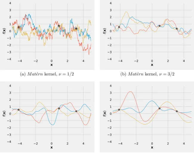
especially simple. Expressions for some of Matérn kernels are given below: kν=1/2(x,x0) = exp(−δ), (2.13) kν=3/2(x,x0) = 1 +√3δexp−√3δ, (2.14) kν=5/2(x,x0) = 1 +√5δ+ 1 3 √ 5δ2 exp(−√5δ), (2.15) kν=7/2(x,x0) = 1 +√7δ+ 2 5 √ 7δ2+ 1 15 √ 7δ3 exp(−√7δ). (2.16) It can be shown that when ν→ ∞ the Matérn kernel becomes squared exponential. In practice, we don’t generally have the prior knowledge about the existence of higher order derivative; so it is probably very difficult to distinguish between values of ν ≥ 7/2 (Rasmussen and Williams, 2006). Fig. 2.3 presents a visualisation of various kernel profiles and sample from posteriors.
Properties of Gaussian processes
There are several reasons for using Gaussian processes for function modelling:
• The posterior distribution can be computed exactly in closed form from kernel functions and some observations. This is rare among Bayesian non-parametric models.
• Taking advantages of the variety of covariance functions, Gaussian processes can express a wide range of functions. The covariance functions can also be combined in Gaussian processes to represent more complex structure of functions.
• Gaussian processes allows us to computemarginal likelihood of the data given a model (MacKay,1992), helping to compare different models for model selection purpose (MacKay and Mac Kay, 2003; Rasmussen and Ghahramani, 2001;
Duvenaud, 2014).
• Using Gaussian processes, overfitting problem is less of an issue since only few parameters need to be estimated (compare to neural networks for example).
4 2 0 2 4
x
4 3 2 1 0 1 2 3 4 f(x
)(a)M at´ernkernel,ν = 1/2
4 2 0 2 4
x
4 3 2 1 0 1 2 3 4 f(x
)(b)M at´ernkernel, ν= 3/2
4 2 0 2 4
x
4 3 2 1 0 1 2 3 4 f(x
)(c)M at´ernkernel,ν= 5/2
4 2 0 2 4
x
4 3 2 1 0 1 2 3 4 f(x
)(d) Squared exponential kernel
Figure 2.3: Example of various kernel profiles sampled from a Gaussian process posterior. Note that when ν increases, the function samples become smoother.
• The computational complexity of matrix inversion in Eq. (2.9) and Eq. (2.10) is O(t3), making exact computation of predictions slow for number of
ob-servations greater than a thousand. This problem can be overcome by using approximate inference methods (Hensman et al.,2013;Quiñonero-Candela and Rasmussen, 2005).
2.4.2
Random forests
Random forest is a standard machine learning technique for classification and re-gression problems (Breiman,2001). Random forest uses decision trees trained from random subsamples of data and averages the predictions of weak learners to produce accurate response surface.
As a surrogate model, random forest regression has been proposed as an express-ive and flexible statistical model for sequential model-based algorithm configuration (SMAC) (Hutter et al., 2011; Shahriari et al., 2016). Since decision tree is flex-ible with various data types, random forest can easily handle categorical data and conditional variables. In addition, because of the scalability and parallelism, ran-dom forest can be readily used for large evaluation budgets which is an advantage compare to the cubic complexity of exact Gaussian process. By subsampling of dimensions to fit decision rule at each iteration, using random forest as surrogate model also helps to deal with high dimensional search spaces (Hutter et al., 2011;
Shahriari et al., 2016).
Using random forest as a surrogate has certain drawbacks. First of all, random forest does not provide the uncertainty in the estimate. Hutter et al. proposed to use empirical variance across the tree predictions as the uncertainty of posterior (Hutter et al.,2011). This heuristic technique might not be accurate, but it has been shown to work well in the context of SMAC. Although being a good predictor for the neighbourhood of training data, random forest is terrible in predicting data points that are far from training data (Shahriari et al., 2016). Indeed, the predictions for those data points are almost identical, resulting in poor prediction (Shahriari et al., 2016). In addition, using variance estimate for the posterior’s uncertainty results in extremely confident intervals. Although Gaussian process is also poor
with extrapolation, it still produces uncertainty for posterior, making it suitable for exploitation and exploration trade-off. Finally, random forest’s response surface is discontinuous and non-differentiable so the acquisition functions using random forest are optimised by a combination of local and random search without using gradient-based methods (Shahriari et al.,2016).
2.4.3
Deep neural networks
Similar to random forest, Bayesian deep neural network is a surrogate model for Bayesian optimisation which provide scalability while maintaining the flexibility and characterisation of uncertainty (Snoek et al., 2015). In (Snoek et al., 2015), the authors proposed a Bayesian optimisation algorithm using deep neural networks called Deep Networks for Global Optimisation (DNGO). The aim of this work is to replace Gaussian process by Bayesian neural networks to retain most of desirable properties of Gaussian process such as flexibility and well-calibrated uncertainty (Snoek et al., 2015). However, since Bayesian neural networks are computationally expensive at large scale, the authors proposed to add a Bayesian linear regressor to the last hidden layer of a deep neural network. Only the output weights of the net are marginalised making the algorithm scale linearly with number of observations and cubically with number of dimensions in basis function (Snoek et al., 2015). For suitable design choice, the author showed that it is possible to create robust and effective Bayesian optimisation system that generalises across many problems (Snoek et al., 2015). The performance of DNGO is shown to be competitive with other GP-based approaches (Snoek et al.,2015).
In another line of work, Springenberg et al. (2016) used Bayesian neural networks to create a robust, scalable and parallel optimiser called Bayesian Optimisation with Hamiltonian Monte Carlo Artificial Neural Network (BOHAMIANN). This algorithm supports both single-task and multi-task optimisation and can be used for high-dimensional optimisation as well as parallel function evaluations. The authors also used scale adaptation technique to improve the robustness of Bayesian inference using stochastic gradient Hamiltonian Monte Carlo (Springenberg et al., 2016).
2.5
Acquisition functions
Thus far, we have discussed about popular probabilistic models used to represent our belief about objective function f at iteration t. We have not described the mechanism for sequentially selecting the next point xt+1 for function evaluation.
Naturally, one can choose an arbitrarily point xt+1 to be evaluated. However, it would be wasteful given information obtained from surrogate models. There is a rich literature that leverages the uncertainty of posterior models to guide the search. In this section, we will focus on the mechanism for selection of next query point xt+1,
often realised by constructing anacquisition function. Fig. 2.4shows some examples of acquisition functions.
The role of the acquisition function is to recommend the next sample for function evaluation. After defining an acquisition function,the original optimisation problem is approached by maximising the acquisition function α as follows:
xt+1 = arg max
x∈X α(x;Dt)
where Dt denotes the data set consists of t observations. Typically, the acquisition
function is defined such that its high value potentially leads to a high value of objective function f. The trade-off between exploring highly uncertain regions or exploiting promising areas is also represented in the acquisition function. Choosing acquisition function is a nontrivial task. In this section, we will discuss several different acquisition functions that have been proposed in the literature. We will first present traditional improvement-based and optimistic approaches, followed by more recent information-based acquisition functions.
2.5.1
Improvement-based policies
Improvement-based acquisition functions suggest points that are likely to improve upon a specific target. Probability of improvement (PI) is an early improvement-based acquisition function in literature proposed by Kushner (1964). This ac-quisition function measures the probability that an input x leads to a function value that is greater than the best function value discovered so far f(x+), where
2 0 2 4 6 8 10
x
2 1 0 1 2f(x)
Target Observations Prediction 95% confidence interval
2 0 2 4 6 8 10 0.0 0.5 1.0
PI
=0.01 =0.1 =1.0 2 0 2 4 6 8 10 0.0 0.2 0.4EI
=0.01 =0.1 =1.0 2 0 2 4 6 8 10 0.0 2.5 5.0UCB
=1 =3 =5Figure 2.4: Examples of acquisition functions. The top plot is the Gaussian model with 3 observations. The remaining plots are the acquisition functions for the Gaus-sian process: PI - Probability Improvement (see Eq. (2.17)), EI - Expected Im-provement (see Eq. (2.19)), UCB - Upper Confidence Bound (see Eq. (2.21)). The yellow triangle makers are the maximum of the acquisition functions.
x+ = argmax
xi∈x1:tf(xi). Since the posterior of the objective functionf is Gaussian,
the probability of improvement acquisition function can be analytically computed as follows: αP I(x;Dt) = P f(x)≥f(x+) = Φ µ(x)−f(x +) σ(x) ! where Φ(x) = √1 2π x −∞e −z2/2
dzis the standard normal cumulative distribution func-tion. This acquisition function prefers points that have a high probability of being greater than f(x+) rather than points that might return larger gain but having
higher uncertainty. In other words, probability of improvement acquisition function is highly exploitative. One can overcome this issue by adding a trade-off parameter
ξ ≥0: αP I(x;Dt) = P f(x)≥f(x+) +ξ = Φ µ(x)−f(x +)−ξ σ(x) ! . (2.17)
As recommended by Kushner, ξ can be set fairly high early in the optimisation to encourage exploration and decreased toward zero as the optimisation continues. The empirical impact of different values of parameter ξ has been studied in several domains (Jones, 2001;Lizotte, 2008).
An alternative approach is to maximise the expected improvement (EI) that involves the improvement function defined by Mockus et al. (1978) as follows:
I(x) = maxn0, ft+1(x)−f(x+)
o
. (2.18)
The probability of the improvement function I(x) can be computed from the density function of the normal distribution N(µ(x), σ2(x)) as:
P (I(x)) = √ 1 2πσ(x)exp " −(µ(x)−f(x +)−I)2 2σ2(x) # .
αEI(x;Dt) = E[I(x)] = I=∞ I=0 I √ 2πσ(x)exp " −(µ(x)−f(x +)−I)2 2σ2(x) # dI.
This integral can be evaluated analytically (Mockus et al.,1978;Jones et al.,1998), yielding the following results:
αEI(x;Dt) = zσ(x)Φ(z) +σ(x)φ(z) if σ(x