Robust Algorithms for Low-Rank and Sparse Matrix Models

(1)

Robust Algorithms for Low-Rank and Sparse

Matrix Models

by Brian E. Moore

A dissertation submitted in partial fulfillment of the requirements for the degree of

Doctor of Philosophy (Electrical Engineering: Systems)

in The University of Michigan 2018

Doctoral Committee:

Associate Professor Raj Rao Nadakuditi, Chair Professor Jeffrey A. Fessler

Professor Alfred O. Hero III Assistant Professor Shuheng Zhou

(2)

Brian E. Moore [email protected] ORCID iD: 0000-0001-7914-1794

c

(3)

(4)

ACKNOWLEDGEMENTS

I would first like to thank my advisor Prof. Raj Nadakuditi. Thank you for your guidance, your support, and your endless supply of creative research ideas. You gave me direction when I needed it, empowered me to pursue projects when the opportunities arose, and exposed me to many interesting concepts that I would not have encountered otherwise. I admire your enthusiasm for your work and your “why not?” mentality; this mindset has rubbed off on me—both in research and life—and compelled me to pursue my passions with confidence. I am especially grateful for our flexible working relationship that allowed me to work remotely over the last year as I moved to be with my wife. It was a pleasure to have been in your group, and I look forward to continued work on our untapped projects!

I would also like to thank the rest of my committee—Prof. Jeff Fessler, Prof. Al Hero, and Prof. Shuheng Zhou—for their mentorship and invaluable feedback through-out my dissertation work. Prof. Fessler, thank you for adopting me as a de facto mem-ber of your research group. Your passion for your work is infectious, and I greatly admire your unique blend of professionalism and attentiveness to your students. I learned much from you about optimization, and I appreciate your input on our nu-merous collaborations. You have significantly and positively impacted this thesis. Prof. Hero, thank you as well for your valuable guidance and feedback on my work. Your vast knowledge of signal processing and data science was a great resource. I even learned from you during my qualification exam when you were supposed to be evaluating me! Prof. Zhou, thank you for your flexibility and willingness to join my committee. I particularly enjoyed our conversations about statistical signal estima-tion, which provided some valuable context for our work on robust PCA theory.

Thank you to Sai, Andrew, Chen, and Raj Tejas for our enjoyable and fruitful collaborations. Working with you was truly a pleasure, and I am proud of the research we produced together. Thank you also to Curtis, Nick, Arvind, Madison, Gopal, David, and the other members of the Nadakuditi and Fessler research groups for the many stimulating discussions about research, coursework, current events, philosophy, logic puzzles, and general socializing that made our time in the office enjoyable.

(5)

Lastly—and most importantly—thank you to my wife Meriah for your uncondi-tional love and support. Thank you for enduring a temporary long distance relation-ship as we pursued our educations; I am thrilled for our future together. This work is dedicated to you.

(6)

LIST OF FIGURES

Figure

2.1 Singular values of acn×n matrix with i.i.d. Gaussian entries for two values ofn. Left: singular value scree plots. Right: empirical singular value historgrams. The red curve denotes the limiting Marcenko-Pastur law (2.10). . . 10 2.2 Singular value spectrum ofXe_ndrawn from the model (2.5) withr = 3

and {θ1, θ2, θ3} = {4, 3, 2}. The noise Xn is drawn from the Marcenko-Pastur law with τ = 1. The blue X’s denote the singular values of Xe_n, the blue curve denotes their empirical histogram, and the red curve is the limiting spectrum predicted by Theorem II.1. All three signals are above the critical pointκ= 1, so the location of the extreme singular values are asymptotically given byρi =D−1µX(1/θ

2

i), for i= 1,2,3. . . 11 2.3 Singular value spectrum ofXe_ndrawn from the model (2.5) withr = 3

and {θ1, θ2, θ3} = {4, 3, 0.95}. The noise Xn is drawn from the Marcenko-Pastur law with τ = 1. The blue X’s denote the singular values of Xe_n, the blue curve denotes their empirical histogram, and the red curve is the limiting spectrum predicted by Theorem II.1. The third signal θ3 = 0.95 is less than the critical point κ = 1, so it does not separate from the bulk spectrum. . . 11 3.1 Two representative frames from the decompositions produced by the

proposed method (3.11) and the SVT-based method (3.8) on the Fountain sequence with parameters δ = 0.0025, τk = 0.5, ps = 0.15, andK = 0.5. The row labelsLandS denote the low-rank and sparse components, respectively, returned by each algorithm. The column labels denote the frame number (i.e., column ofLand S) that is dis-played. Each panel is displayed on the same intensity scale. NRMSE values are reported for the low-rank components using output of the SVT-based updates with ps = 0 as ground truth. . . 23 3.2 Example coil sensitivities for the cardiac perfusion data from [1]. . . 24 3.3 Examplek-space sampling masks for the cardiac perfusion data from [1]. 24

(12)

3.4 Four representative frames from the reconstructions on the cardiac perfusion dataset from [1]. The columns of each panel show the final reconstruction ˆL + ˆS, the low-rank component ˆL, and the sparse component ˆS, respectively, produced by each method. . . 25 3.5 Four representative frames from the reconstructions on the cardiac

perfusion dataset from [2, 3]. The columns of each panel show the final reconstruction ˆL+ ˆS, the low-rank component ˆL, and the sparse component ˆS, respectively, produced by each method. . . 27 4.1 The video registration process. The top row depicts raw video frames

Fk with SURF features annotated. The bottom row depicts the cor-responding registered framesFe_kcomputed via (4.5). Thekth column of the mask matrixM ∈ {0,1}mn×p _{encodes the support of}

e

Fkwithin the aggregate view; i.e., Mik = 0 for unobserved pixels, which are represented by white space in the registered frames above. . . 33 4.2 Summary of the proposed PRPCA algorithm. . . 46 4.3 A representative frame from the decompositions produced by each

method applied to the Hall sequence corrupted by 30 dB Gaussian noise. Left column: observations; L: reconstructed background; S: reconstructed foreground; L+S: reconstructed scene; right column: Hall sequence. . . 49 4.4 A representative frame from the decompositions produced by each

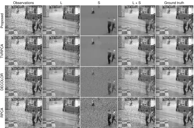
method applied to the Water Surface sequence corrupted by 20% outliers. Left column: observations; L: reconstructed background;

S: reconstructed foreground; L+S: reconstructed scene; fifth col-umn: Water Surface sequence; F: estimated foreground mask; right column: true mask. . . 50 4.5 A representative frame from the decompositions produced by each

method applied to the Water Surface sequence with 70% missing data. Left column: observations; L: reconstructed background; S: reconstructed foreground;L+S: reconstructed scene; Fifth column: original Water Surface sequence; F: foreground mask estimated by optimally thresholding S; right column: true foreground mask. . . . 50 4.6 Three representative frames from the decomposition produced by the

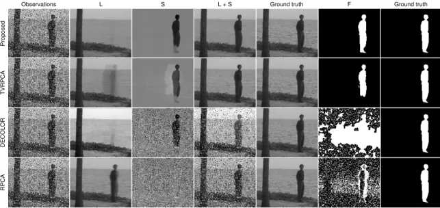
proposed PRPCA method applied to the Tennis sequence corrupted by 30% salt and pepper outliers. Left column: registered observa-tions; L: reconstructed registered background;S: reconstructed reg-istered foreground; L+S: reconstructed registered scene restricted to the current field of view; right column: registered Tennis sequence. 53 4.7 The decompositions from Figure 4.6 mapped to the perspective of

(13)

4.8 Three representative frames from the decomposition produced by the proposed PRPCA method applied to the Tennis sequence corrupted by 70% missing data. Left column: registered observations; L: re-constructed registered background; S: reconstructed registered fore-ground;L+S: reconstructed registered scene restricted to the current field of view; right column: registered Tennis sequence. . . 54 4.9 The decompositions from Figure 4.8 mapped to the perspective of

the original video . . . 54 4.10 Two representative frames from decompositions of the Paragliding

sequence corrupted by 10 dB Poisson noise. Top row: decomposi-tion produced by the proposed PRPCA method mapped to the per-spective of the original video; bottom row: decomposition produced by DECOLOR. Left column: observations; L: reconstructed back-ground; S: reconstructed foreground; L+S: reconstructed scene; right column: Paragliding sequence. . . 55 4.11 Per-iteration convergence of theL,E, andS components of the

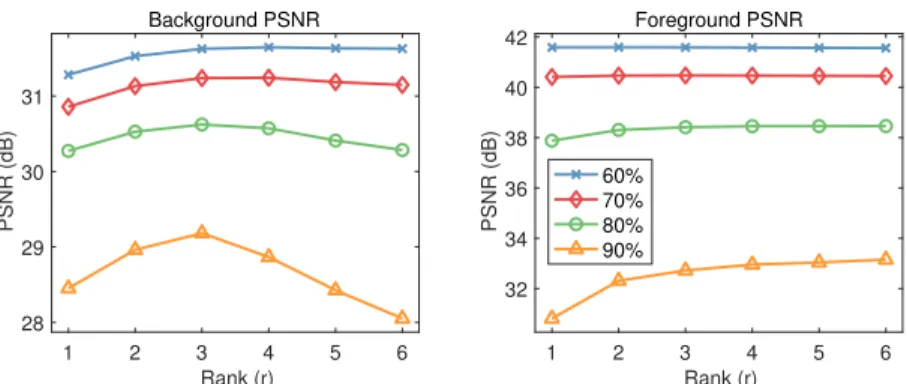
pro-posed PRPCA method on the Fountain sequence corrupted by out-liers at various percentages. . . 55 4.12 Foreground and background PSNRs as a function of OptShrink rank

parameterron the Tennis sequence for various missing data percent-ages. . . 56 5.1 Graphical depiction ofshrinkτ,λ for various values ofλ. Note that it

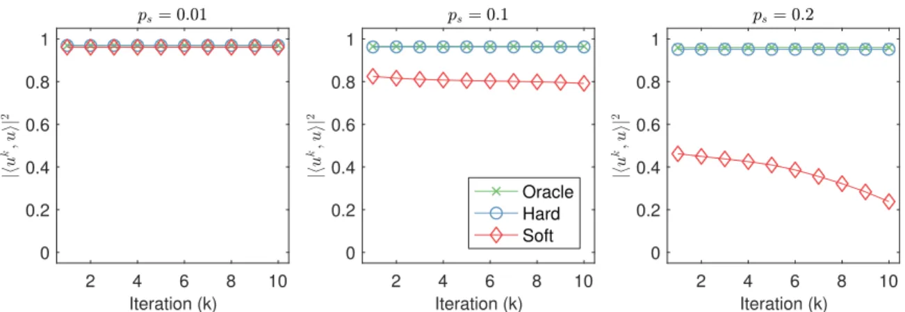
reduces to hard tresholding when λ = 0 and reduces to soft thresh-olding when λ=τ. . . 67 5.2 Empirical validation of Theorem V.8. The left figure plots the first

right singular vector accuracy |hv1,ev1i|

2

of the estimators Xe? (ora-cle), Xe_τHT (hard), Xe_τST (soft), and Xe (PCA) as a function of outlier probabilityps. The remaining figures plot (from left to right) the first right singular vectors of Xe?,Xe_τHT, andXe_τST reshaped into images for the particular choice ofps= 15% denoted by the solid markers in the left figure. . . 69 5.3 Accuracy of the first left singular vector uk of the low-rank updates

Lk_{from (5.29) and (5.30) as a function of iteration. Each panel} corre-sponds to a different outlier probability ps. The three curves in each panel depict the performance of the variations of alternating mini-mization where the S-updates are performed using hard thesholding (Hard), soft thresholding (Soft), and the oracle sparse estimator (Or-acle) that inserts zeros at the known outlier locations. . . 72 6.1 Images: Barbara, Boat, Hill, and a Microscopy image. . . 80 6.2 Algorithm behavior: Objective function (top left); NSRE (top right);

normalized changes between successive DiterateskDt−Dt−1kF/

√

J

(bottom left); and normalized changes between successive C iterates

kCt₋_Ct−1_k

(14)

6.3 8x undersampling: Frames 7 and 13 of the proposed DINO-KAT MRI (r= 1) reconstruction along with the reference frames. . . 84 7.1 Flowchart of the proposed online adaptive dictionary learning

alter-nating update scheme at time t. The input is a vector yt contain-ing the streamcontain-ing measurements for the current minibatch, and xt denotes the corresponding reconstructed frames. In the dictionary learning step, (D, Ct) are updated with xt held fixed by performing block coordinate descent over the columns ofCt_(the_{dictioanry atom}

update) and the columns of D (the sparse coding step). Then, the

framesxtare updated (theimage update step) with (D, Ct) held fixed. This process is repeated a few times, and the final frame estimates ˆ

xt are integrated into the streaming reconstruction, ˆx. . . 92 7.2 Two representative frames from the reconstructions produced by each

method on the Coastguard video with 80% missing pixels (top) and 80% pixels with 25 dB Gaussian noise added (bottom). The methods considered are the proposed online DINO-KAT learning method (r = 5), the online method with fixed DCT dictionary, the batch DINO-KAT learning method, and 3D interpolation. Top: the proposed method method achieves PSNR improvements of 2.0 dB, 1.0 dB, and 1.4 dB, respectively, compared to the other methods. Bottom: the proposed method achieves PSNR improvements of 1.0 dB, 1.0 dB, and 1.5 dB, respectively, compared to the other methods. . . 100 7.3 Two representative frames from the reconstructions produced by each

method on the Flower Garden video with 80% missing pixels. The methods considered are the proposed online DINO-KAT learning method (r = 5), the online method with fixed DCT dictionary, the batch DINO-KAT learning method, and 3D interpolation. The pro-posed method achieves PSNR improvements of 0.7 dB, 0.6 dB, and 1.3 dB, respectively, compared to the other methods. . . 101 7.4 Per-frame PSNR for the reconstructions produced by each method

on the Coastguard video with 70% missing pixels (left) and the Bus video with 50% missing pixels (right). The methods considered are the proposed online DINO-KAT learning method (r = 5), the pro-posed online method with unitary dictionary, the online method with fixed DCT dictionary, the batch DINO-KAT learning method, and 3D interpolation. . . 101 7.5 Dictionaries for the Bus video with 50% missing pixels. Top: the

initial DCT dictoinary; bottom: the learned dictionary produced by the proposed online DINO-KAT learning method with r = 5. Left: the first 8×8 slice of each atom; right: the y−t profiles of a vertical cross-section through each 8×8×5 tensor. . . 102

(15)

7.6 Two representative frames from a reference (fully sampled) recon-struction along with the corresponding frames from the proposed online DINO-KAT learning-based reconstruction on the cardiac per-fusion data with 12x undersampling (Cartesian sampling). The right four columns depict the corresponding reconstruction error maps (w.r.t. reference) for the proposed online DINO-KAT learning method, the online method with fixed DCT dictionary, the k-t SLR method, and the L+S method, respectively. The proposed online method achieves NRMSE improvements of 0.6 dB, 1.9 dB, and 0.7 dB, re-spectively, compared to the other methods. . . 105 7.7 Two representative frames from a reference (fully sampled)

recon-struction along with the corresponding frames from the proposed online DINO-KAT learning-based reconstruction on the PINCAT data with 7x undersampling (pseudo-radial sampling). The right four columns depict the corresponding reconstruction error maps (w.r.t. reference) for the proposed online DINO-KAT learning method, the online method with fixed DCT dictionary, the k-t SLR method, and the L+S method, respectively. The proposed online method achieves NRMSE improvements of 0.4 dB, 1.0 dB, and 2.3 dB, re-spectively, compared to the other methods. . . 106 7.8 Per-frame PSNR for the reconstructions produced by each method on

the PINCAT data with 9x undersampling (pseudo-radial sampling). The methods shown are the proposed online DINO-KAT learning method, the online method with fixed DCT dictionary, the k-t SLR method, and the L+S method. . . 106 7.9 Temporal (y−t) profiles of a spatial vertical line cross section for the

reference PINCAT reconstruction, the proposed online DINO-KAT learning method, the online method with fixed DCT dictionary, the k-t SLR mek-thod, and k-the L+S mek-thod for 14x undersampling (pseudo-radial sampling). . . 107 7.10 Dictionaries for the PINCAT data with 9x undersampling. Left: the

atoms of the initial DCT dictionary. Right: the real and imagi-nary parts of the learned dictioimagi-nary produced by the proposed online DINO-KAT learning method with r = 1. The dictionary atoms are 8×8×5 tensors, so only the first 8×8 slice of each atom is displayed.108 8.1 The LASSI reconstruction algorithms for Problems (P1) and (P2),

(16)

8.2 Behavior of the LASSI algorithms with Cartesian sampling and 8x undersampling. The algorithms are labeled according to the method used for xL update, i.e., SVT or OptShrink (OPT), and according to the type of sparsity penalty employed for the patch coefficients (`0 or `1 corresponding to (P1) or (P2)). (a) Objectives, shown

only for the algorithms for (P1) and (P2) with SVT-based updates, since the OptShrink-based updates do not correspond to minimiz-ing a formal cost function); (b) NRMSE; (c) Sparsity fraction of Z

(i.e., kZk0/mM) expressed as a percentage; (d) normalized changes

between successive dMRI reconstructions kxt_L+xt_S−xt_L−1−xt_S−1k2/

kxrefk2; (e) real and (f) imaginary parts of the atoms of the learned

dictionaries in LASSI (using`0sparsity penalty and OptShrink-based xL update) shown as patches – only the 8×8 patches correspond-ing to the first time-point (column) of the rank-1 reshaped (64×5) atoms are shown; and frames 7 and 13 of the (g) conventional L+S reconstruction [1] and (h) the proposed LASSI (with `0 penalty and OptShrink-based xL update) reconstruction shown along with the corresponding reference frames. The low-rank (L) and (transform or dictionary) sparse (S) components of each reconstructed frame are also individually shown. Only image magnitudes are displayed in (g) and (h). . . 126 8.3 NRMSE values computed between each reconstructed and reference

frame for LASSI, L+S, and k-t SLR for (a) the cardiac perfusion data [1, 4] at 8x undersampling, and (b) the PINCAT data at 9x undersampling. . . 130 8.4 LASSI reconstructions and the error maps (clipped for viewing) for

LASSI, L+S, and k-t SLR for frames of the cardiac perfusion data [1,4] (first row), PINCAT data [2,5] (second row), andin vivo myocar-dial perfusion data [2, 5] (third row), shown along with the reference reconstruction frames. Undersampling factors (top to bottom): 8x, 9x, and 8x. The frame numbers and method names are indicated on the images. . . 131 8.5 A frame of the reference PINCAT [2, 5] reconstruction is shown (left)

with a spatial line cross section marked in green. The temporal (x−

t) profiles of that line are shown for the reference, LASSI, DINO-KAT dMRI, L+S [1], and k-t SLR [2] reconstructions for pseudo-radial sampling and nine fold undersampling. The NRMSE values computed between the reconstructed and reference x−t profiles are 0.107, 0.116 , 0.153, and 0.131 respectively, for LASSI, DINO-KAT dMRI, L+S, and k-t SLR. . . 132 8.6 A frame of the reference PINCAT [2, 5] reconstruction is shown (left)

with a spatial line cross section marked in green. The temporal (x−

t) profiles of that line are shown for the reference, and the LASSI reconstructions at 5x, 9x, and 27x undersampling and pseudo-radial sampling. . . 132

(17)

8.7 LASSI reconstructions and error maps (clipped for viewing) for frames of the cardiac perfusion data [1,4] at 4x, 12x, and 20x undersampling (Cartesian sampling), shown along with the reference reconstruction frames. The images are labeled with the frame numbers and under-sampling factors. . . 133 8.8 Regions of interest containing the heart shown using green bounding

boxes for a frame of (a) the cardiac perfusion data [1], (b) PINCAT data [2, 5], and (c) in vivo myocardial perfusion MRI data [2, 5], respectively. . . 133 8.9 Study of LASSI models, methods, and initializations at various

un-dersampling factors for the cardiac perfusion data in [1,4] with Carte-sian sampling: (a) NRMSE for LASSI with `0 “norm” for sparsity

and with xL updates based on SVT (p = 1), OptShrink (OPT), or based on the Schatten p-norm (p= 0.5) or rank penalty (p= 0); (b) NRMSE for LASSI with `1 sparsity and with xL updates based on SVT (p = 1), OptShrink (OPT), or based on the Schatten p-norm (p= 0.5) or rank penalty (p= 0); (c) NRMSE for LASSI when ini-tialized with the output of the L+S method [1] (used to initialize xS with x0_L = 0) together with the NRMSE for the L+S method; (d) NRMSE for LASSI when initialized with the output of the k-t SLR method [2] or with the baseline reconstruction (performing zeroth order interpolation at the nonsampled k-t space locations and then backpropagating to image space) mentioned in Section 8.4.1 (these are used to initializexS withx0L= 0), together with the NRMSE val-ues for k-t SLR; (e) NRMSE versus dictionary size at different accel-eration factors; (f) NRMSE improvement (in dB) achieved withr = 1 compared to the r = 5 case in LASSI; (g) NRMSE for LASSI with different dictionary initializations (a random dictionary, a 320×320 1D DCT and a separable 3D DCT of the same size) together with the NRMSEs achieved in LASSI when the dictionary is fixed to its ini-tial value; and (h) NRMSE versus the fraction of nonzero coefficients (expressed as percentage) in the learned Z at different acceleration factors. . . 136 8.10 The normalized sparse representation error (NSRE)kY−DCHkF/kYkF

for the 320×320 dictionaries learned on the 8×8×5 overlapping spa-tiotemporal patches of the fully sampled cardiac perfusion data [1]. The results are shown for various choices of the `0 sparsity penalty parameter λZ corresponding to different fractions of nonzero coef-ficients in the learned C and for various choices of the atom rank parameter r. . . 139 9.1 Mean angular errors (in degrees) of the estimated normal vectors for

the DiLiGenT Cat dataset as a function of number of images used during reconstruction. . . 158

(18)

9.2 Mean angular errors (in degrees) of the estimated normal vectors for the DiLiGenT Harvest dataset as a function of number of images used during reconstruction. . . 158 9.3 Mean angular errors (in degrees) of the estimated normal vectors for

the DiLiGenT Pot2 dataset with 20 images versus SNR. . . 158 9.4 Normal vector reconstructions for the DiLiGenT Pot2 dataset with

20 images and 5 dB Poisson noise. . . 159 9.5 Normal vector error maps (in degrees) for the DiLiGenT Pot2 dataset

with 20 images and 5 dB Poisson noise. . . 159 9.6 Normal vector error maps (in degrees) computed with PDLNV for

the DiLiGenT Cat dataset with 20 images and varying SNR. . . 160 9.7 Mean angular errors (in degrees) of estimated normal vectors for the

Hippo dataset with 20 images versus SNR. . . 161 9.8 Normal vector reconstructions for the Cat dataset with 20 images

and 5 dB Poisson noise. . . 162 9.9 Normal vector error maps (in degrees) for the Cat dataset with 20

images and 5 dB Poisson noise. . . 162 9.10 Surfaces computed from the estimated normal vectors of the Cat

dataset with 20 images and 5 dB Poisson noise. . . 163 9.11 Cost function, normal vector angular errors (in degrees), and sparsity

of the sparse coding matrix B for the PDLNV method with p = 2 applied to the DiLiGenT Cat dataset with 20 images and 20 dB Poisson noise for several different dictionary sizes. . . 165 9.12 Mean angular error (in degrees) of the estimated normal vectors for

PDLNV with multiple values of p on the DiLiGenT Pot1 dataset as a function of number of images used. . . 165 9.13 Initial and final learned dictionaries for the PDLNV method with

p= 2 applied to the full DiLiGenT Pot1 dataset. . . 166 10.1 Reconstructions of the Tent surface with SNR = 20 dB. . . 172 10.2 Reconstructions of the Vase surface with SNR = 30 dB. . . 172 10.4 Surface reconstructions for the Frog dataset with SNR = 17 dB. . . 174 D.1 Illustration of the notation defined in Section D for two possible

out-lier distributions. . . 188 D.2 Graphical depiction of (∆HT_X )ij as a function ofGij+Sij for two fixed

values of Lij. . . 191 E.1 Graphical depiction of (∆ST

X )ij as a function of Gij+Sij for two fixed values of Lij. . . 203

(19)

LIST OF TABLES

Table

3.1 NRMSE values as percentages for reconstructions of the cardiac per-fusion data from [1] as a function of retrospective noise varianceC/n2

p. The best NRMSE for each trial is in bold. . . 26 3.2 NRMSE values in percent for reconstructions of the cardiac perfusion

data from [2, 3] as a function of retrospective noise variance C/n2

p. The best NRMSE for each setting is in bold. . . 27 4.1 Performance metrics for each method on sequences from the I2R

dataset corrupted by 20% outliers. . . 47 4.2 Performance metrics for each method on sequences from the I2R

dataset corrupted by 30 dB Gaussian noise. . . 48 4.3 Performance metrics for each method on sequences from the I2R

dataset corrupted by 70% missing data. . . 48 4.4 Performance metrics for each method on the Hall sequence as a

func-tion of outlier probability. . . 48 4.5 Performance metrics for each method on the Hall sequence as a

func-tion of SNR (Gaussian noise). . . 48 4.6 Performance metrics for each method on the Hall sequence as a

func-tion of missing data probability. . . 48 4.7 Performance metrics for each method on sequences from the DAVIS

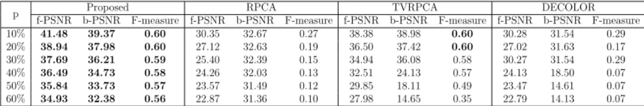
dataset corrupted by 30% outliers. *DECOLOR raises an error when run on the Tennis sequence due to the significant camera motion, so it is omitted. . . 49 4.8 Performance metrics for each method on sequences from the DAVIS

dataset corrupted by 10 dB Poisson noise. . . 51 4.9 Performance metrics for each method on sequences from the DAVIS

dataset corrupted by 70% missing data. . . 51 4.10 Performance metrics for each method on the Tennis sequence as a

function of outlier probability. DECOLOR raises an error when run on the Tennis sequence due to the significant camera motion, so it produces no decompositions. . . 51 4.11 Performance metrics for each method on the Tennis sequence as a

(20)

4.12 Performance metrics for each method on the Tennis sequence as a function of missing data probability. . . 51 5.1 Effective SNRs for Theorem V.8 . . . 66 6.1 Inpainting PSNR values in decibels (dB) at various percentages of

measured pixels for the initial image, the result with cubic interpo-lation, the results using (P2) with r = 1, r = 2, r = 3, and r = 8, and for the reconstructions obtained with fixed dictionary in our al-gorithm. Results are for the Microscopy image. The best PSNRs are marked in bold. . . 82 6.2 NRMSE values at several undersampling factors for the L+S method

and for the algorithm for (P2) with r= 5 (full rank), r = 1 (DINO-KAT MRI) and fixed dictionary cases. The best NRMSE values for each undersampling are marked in bold, and the improvements by DINO-KAT MRI are indicated in decibels (dB). . . 83 7.1 PSNR values in decibels (dB) for video inpainting on three videos

from the BM4D dataset at various percentages of missing pixels. The methods considered are the proposed online DINO-KAT learn-ing method with r = 5, the proposed online method with unitary dictionary, online inpainting with a fixed DCT dictionary, the batch DINO-KAT learning method with r= 5, 2D (frame-by-frame cubic) interpolation, and 3D interpolation The best PSNR for each under-sampling on each video is in bold. . . 98 7.2 PSNR values in decibels (dB) for video inpainting on the Coastguard

video corrupted by Gaussian noise with 25dB PSNR at various per-centages of missing pixels. The methods considered are the proposed online DINO-KAT learning method with r = 5, the proposed on-line method with unitary dictionary, the batch DINO-KAT learning method with r = 5, online inpainting with a fixed DCT dictionary, 2D (frame-by-frame cubic) interpolation, and 3D interpolation The best PSNR for each undersampling is in bold. . . 99 7.3 Left: NRMSE values as percentages for the cardiac perfusion data

at several undersampling factors with Cartesian sampling. Right: NRMSE values as percentages for the PINCAT data at several under-sampling factors with pseudo-radial under-sampling. The methods consid-ered are the proposed online DINO-KAT learning method withr= 1, the online scheme with fixed DCT dictionary, the batch DINO-KAT learning method with r= 1, the L+S method, the k-t SLR method, and a baseline reconstruction. The best NRMSE for each undersam-pling on each dataset is in bold. . . 105

(21)

7.4 NRMSE values as percentages for the cardiac perfusion data at sev-ersal undersampling factors with Cartesian sampling. The methods considered are the online scheme with a fixed dictionary learned from patches of a reference reconstruction, the proposed online DINO-KAT learning method with two passes over the frames, the proposed on-line DINO-KAT learning method with a single pass over the frames, the proposed online method with unitary dictionary, and the online scheme with fixed DCT dictionary. The best NRMSE for each un-dersampling is in bold. . . 107 8.1 NRMSE values expressed as percentages for the L+S [1], k-t SLR [2],

and the proposed DINO-KAT dMRI and LASSI methods at sev-eral undersampling factors for the cardiac perfusion data [1, 4] with Cartesian sampling. The NRMSE gain (in decibels (dB)) achieved by LASSI over the other methods is also shown. The best NRMSE for each undersampling factor is in bold. . . 128 8.2 NRMSE values expressed as percentages for the L+S [1], k-t SLR [2],

and the proposed DINO-KAT dMRI and LASSI methods at several undersampling factors for the PINCAT data [2, 5] with pseudo-radial sampling. The best NRMSE values for each undersampling factor are marked in bold. . . 129 8.3 NRMSE values expressed as percentages for the L+S [1], k-t SLR [2],

and the proposed DINO-KAT dMRI and LASSI methods at several undersampling factors for the myocardial perfusion MRI data in [2, 5], using pseudo-radial sampling. The best NRMSE values for each undersampling factor are marked in bold. . . 130 8.4 NRMSE values for an ROI (Figure 8.8(a)) in the cardiac perfusion

data [1] expressed as percentages for the L+S [1], k-t SLR [2], and the proposed DINO-KAT dMRI and LASSI methods at several un-dersampling factors and Cartesian sampling. The best NRMSE value at each undersampling factor is indicated in bold. . . 134 8.5 NRMSE values for an ROI (Figure 8.8(b)) in the PINCAT data [2, 5]

expressed as percentages for the L+S [1], k-t SLR [2], and the pro-posed DINO-KAT dMRI and LASSI methods at several undersam-pling factors and pseudo-radial samundersam-pling. The best NRMSE value at each undersampling factor is indicated in bold. . . 134 8.6 NRMSE values for an ROI (Figure 8.8(c)) in the myocardial perfusion

MRI data [2, 5] expressed as percentages for the L+S [1], k-t SLR [2], and the proposed DINO-KAT dMRI and LASSI methods at several undersampling factors and pseudo-radial sampling. The best NRMSE value at each undersampling factor is indicated in bold. . . 134 9.1 Mean angular errors of the estimated normal vectors for the full,

uncorrupted DiLiGenT datasets. . . 156 10.1 Quality of Tent (left) and Vase (right) surface reconstructions in

(22)

LIST OF APPENDICES

Appendix

A. Incorporating Missing Data into Existing Foreground-Background Sep-aration Algorithms . . . 179 B. Useful Results for Appendices C, D, and E . . . 184 C. Proof of Theorem V.7 . . . 185 D. Proof of Theorem V.8 for Hard Thresholding . . . 187 E. Proof of Theorem V.8 for Soft Thresholding . . . 200

(23)

ABSTRACT

Data in statistical signal processing problems is often inherently matrix-valued, and a natural first step in working with such data is to impose a model with structure that captures the distinctive features of the underlying data. Under the right model, one can design algorithms that can reliably tease weak signals out of highly corrupted data. In this thesis, we study two important classes of matrix structure: low-rankness and sparsity. In particular, we focus on robust principal component analysis (PCA) models that decompose data into the sum of low-rank and sparse (in an appropriate sense) components. Robust PCA models are popular because they are useful models for data in practice and because efficient algorithms exist for solving them.

This thesis focuses on developing new robust PCA algorithms that advance the state-of-the-art in several key respects. First, we develop a theoretical understanding of the effect of outliers on PCA and the extent to which one can reliably reject outliers from corrupted data using thresholding schemes. We apply these insights and other recent results from low-rank matrix estimation to design robust PCA algorithms with improved low-rank models that are well-suited for processing highly corrupted data. On the sparse modeling front, we use sparse signal models like spatial continuity and dictionary learning to develop new methods with important adaptive representational capabilities. We also propose efficient algorithms for implementing our methods, in-cluding an extension of our dictionary learning algorithms to the online or sequential data setting. The underlying theme of our work is to combine ideas from low-rank and sparse modeling in novel ways to design robust algorithms that produce accurate reconstructions from highly undersampled or corrupted data. We consider a variety of application domains for our methods, including foreground-background separa-tion, photometric stereo, and inverse problems such as video inpainting and dynamic magnetic resonance imaging.

(24)

CHAPTER I

Introduction

Data in statistical signal processing problems is often inherently matrix-valued. For example, in the canonical Netflix problem, one is interested in completing a large, highly undersampled matrix whose rows represent users, columns represent movies, and entries represent movie ratings. A natural first step in working with matrix-valued data is to impose some structure to make the desired task (estimation, detection, etc.) tractable. In this thesis, we focus on two important classes of matrix structure: low-rankness and sparsity.

1.1 Low-Rank and Sparse Matrix Models

Low-rank matrices arise in statistical signal processing problems for many rea-sons. In practice, low-rankness allows for dimensionality reduction, which is often an essential preprocessing step when working with high dimensional data. Low-rankness is also important from a theoretical perspective because it implies that the data has some inherent redundancy that can be leveraged to reliably tease weak signals out of highly corrupted data. Perhaps the most algorithm for low-rank models is principal component analysis (PCA). In PCA, one estimates the latent low-rank structure of a high-dimensional dataset by computing the subspace spanned by the first few sin-gular vectors of the data. Obtaining an accurate estimate of the underlying subspace is critically important to the success of subsequent inferential tasks. Although PCA is stable in the presence of relatively small noise, it is well-known that even a few large outliers in the data can cause PCA to breakdown completely. In this thesis, we contribute both theoretical understanding of the breakdown of PCA in the presence of outliers and algorithms to avoid this breakdown in practice.

Sparsity is another fundamental property of many datasets. Data may exhibit sparsity in many forms. It may simply contain few non-zero elements, i.e., have

(25)

sparse support; it may exhibit spatial or temporal continuity, i.e., be sparse in a total variation sense;, or it may be sparse with respect to a more general fixed or adap-tive transformation, i.e., as in dictionary learning. Each of these sparsity models will play an important role in this thesis. Depending on the application, the sparsity of a dataset can be an asset or a liability. For example, in conventional PCA, sparse corruptions are a nuisance that conspire to destroy the subspace estimate. However, in other applications—such as foreground-background separation and dynamic med-ical imaging, which we will consider in this thesis—sparsity may capture the critmed-ical dynamic features of the dataset that have physical meaning and importance.

Recently there has been great interest in methods that decompose data into low-rank and sparse (in an appropriate sense) components. These so-called robust PCA models are popular because they are useful models for data in practice and because simple algorithms exist for solving them. The bulk of this thesis is dedicated to developing new robust PCA algorithms that advance the state-of-the-art in several key aspects. On the low-rank front, we apply theoretical results from low-rank matrix estimation to design robust PCA algorithms with improved low-rank models. On the sparsity front, we develop new methods that exploit sparse signal models like spatial continuity and adaptive transform sparsity to achieve best-in-class results on practical problems in computer vision and inverse problems. The underlying theme of this work is to combine ideas from low-rank and sparse modeling in novel ways to design robust algorithms that produce accurate reconstructions from highly undersampled or corrupted data.

1.2 Contributions

The rest of this thesis is organized as follows. Chapter II briefly provides some common groundwork and motivation for our investigation, but the subsequent chap-ters are intended to be mostly self-contained.

In Chapter II, we present some background on the problem of estimating a low-rank matrix corrupted by noise. This fundamental problem underlies all of the robust PCA methods discussed in this thesis, because each algorithm uses an alternating minimization scheme where one step of the problem can be thought of as a low-rank matrix denoising step. We review the prevailing low-rank estimation methods in the literature, and then we present some recent theoretical results from random matrix theory on optimal low-rank matrix estimation that culminates in OptShrink, a recent data-driven low-rank matrix estimator that we employ throughout this thesis.

(26)

In Chapter III, we study the robust PCA problem of reliably recovering a low-rank signal matrix from a signal-plus-noise-plus-outliers matrix. We begin by analytically characterizing the effect of outliers on the data matrix, and we discuss why recent classical robust PCA algorithms will produce suboptimal low-rank matrix estimates in the presence of noise. Then we propose a new robust PCA algorithm that leverages OptShrink to improve low-rank matrix estimation quality. We demonstrates the state-of-the-art performance of our proposed method on a background subtraction task from computer vision and highly accelerated dynamic magnetic resonance imaging (MRI) reconstruction. This chapter is based on [6, 7].

In Chapter IV, we extend our work on background subtraction from Chapter III to the general case of foreground-background separation on freely moving camera video with dense and sparse corruptions. We propose a method that can produce a panoramic background component that automatically stitches together corrupted data from partially overlapping frames to reconstruct the full field of view, and we use a weighted total variation framework that enables our method to reliably decouple the true foreground of the video from sparse corruptions. We perform extensive numerical experiments on both corrupted static and moving camera video that demonstrate the state-of-the-art performance of our proposed method compared to existing methods both in terms of foreground and background estimation accuracy. This chapter is based on [8, 9].

Next, we take a theoretical aside and consider the problem of recovering a low-rank matrix corrupted by random noise and outliers in Chapter V. Motivated by the sparse estimation literature, we consider outlier rejection schemes that apply hard or soft thresholding, respectively, to the elements of the data matrix. We analyze the accuracy of the low-rank matrix estimated by applying PCA to the outlier-rejected data by comparing it to an oracle estimator that replaces the known outlier-corrupted entries of the data matrix with zeros. Our analysis reveals a surprising result: in the dense outlier regime, the hard thresholding-based estimator achieves oracle accuracy while the soft thresolding-based estimator breaks down completely. This is an in-teresting result because in the context of sparse signal estimation, hard and soft thresholding both exhibit similar performance. This chapter is based on [10, 11].

In Chapter VI, we shift our focus to sparse signal models based on adaptive dictionary learning. Traditional dictionary learning problems are non-convex and NP-hard, and the usual alternating minimization approaches for learning are often expensive and lack convergence guarantees. In this chapter, we investigate efficient methods for learning synthesis dictionaries with low-rank atoms. We propose a block

(27)

coordinate descent algorithm for our dictionary learning model that involves efficient updates, and we provide a convergence analysis of the proposed method. Finally, we provide numerical experiments that demonstrate the usefulness of our schemes for highly accelerated dynamic MRI reconstruction and video inpainting. This chapter is based on [12].

We extend our structured dictionary learning framework to the online setting in Chapter VII. In particular, we adapt our model from Chapter VI to process streaming images from a dynamic image sequence in minibathces. At each step, we jointly estimate the underlying images, a dictionary that adapts to all previous data, and the associated sparse coefficients of the model. Our proposed online algorithm involves efficient memory usage and simple and efficient updates of the images, low-rank atoms, and sparse coefficients. Our numerical experiments demonstrate the compelling performance of our algorithm in inverse problem settings, including video reconstruction from noisy, subsampled pixels and highly accelerated dynamic MRI reconstruction. This chapter is based on [13–15].

In Chapter VIII, we integrate our previous work on robust PCA and dictionary learning models into a single low-rank and adaptive sparse framework for highly ac-celerated dynamic imaging applications. Our model decomposes the temporal image sequence into a low-rank component and a component whose spatiotemporal (3D) patches are sparse in an adaptive dictionary domain. We investigate various formu-lations and efficient methods for jointly estimating the underlying dynamic signal components and the spatiotemporal dictionary from limited measurements. Our nu-merical experiments once again demonstrate the promising performance our proposed methods for highly accelerated dynamic MRI reconstruction. This chapter is based on [16, 17].

We return to computer vision in Chapter IX, where we apply adaptive dictionary learning models to the problem of robust photometric stereo. Photometric stereo is a method for reconstructing the normal vectors of an object from a set of images of the object under varying lighting conditions. Classical photometric stereo relies on a diffuse surface model that cannot handle objects with complex reflectance patterns, and it is sensitive to non-idealities in the images. In this chapter, we leverage our dictionary learning models from Chapter VI to develop three new models for photo-metric stereo that are robust to corruptions in the images. Specifically, we propose a preprocessing step that utilizes dictionary learning to denoise the images. We also present a model that applies dictionary learning to regularize and reconstruct the normal vectors from the images under the classic Lambertian reflectance model. We

(28)

then generalize the latter model to explicitly model non-Lambertian objects. This chapter is based on [18, 19].

Finally, in Chapter X, we apply our adaptive dictionary learning framework the problem of robustly reconstructing a surface from imperfect estimates of its normal vectors. Our model simultaneously integrates the gradient fields while sparsely rep-resenting the spatial patches of the reconstructed surface in an adaptive dictionary domain. We show that our formulation learns the underlying structure of the surface, effectively acting as an adaptive regularizer that enforces a smoothness constraint on the reconstructed surface. We revisit the photometric stereo problem from Chapter IX by applying our algorithm to robustly reconstruct a surface from photometric stereo normal vectors, which completes the story of performing robust surface reconstruction from possibly corrupted images of an object. This chapter is based on [20].

(29)

CHAPTER II

Background

This chapter provides a brief background on low-rank matrix models and intro-duces some recent results on low-rank matrix estimation from the random matrix theory literature that will play an important role throughout this thesis.1

2.1 Low-Rank Matrix Models

Suppose we have an arbitrary matrixXe that contains—in a vague sense for now— a low-rank matrix L of known rank r. One of the most basic estimators of L is the truncated singular value decomposition (TSVD) of Xe:

TSVDr(Xe) := r X i=1 e σieuiev H i , (2.1)

where Xe =UeΣeVeH is the SVD ofXe with singular values{σ_e_i}. The TSVD has many interpretations. For example, it is closely related to the ubiquitous principal compo-nent analysis (PCA) [21, 22], where one computes the rank-r subspace in which the data Xe has maximum variance. Alternatively, the well-known Eckart-Young theo-rem [23] asserts that TSVDr(Xe) is the closest rank-r matrix to Xe in the Frobenius norm sense. In other words, it is the solution to the rank-constrained optimization problem min X kXe−Xk 2 F s.t. rank(X)≤r. (2.2)

Thanks in part to the recent explosion of convex optimization, another popular

1_{Random matrix theory is a fascinating and deeply rooted area of mathematics. Here we present}

a brief selection of results that are relevant to this thesis, but each topic merits considerable further attention from an interested reader.

(30)

tool for estimatingL is the singular value thresholding (SVT) estimator [24]: SVTτ(Xe) := X i (_eσi−τ)+euiev H i , (2.3)

where τ >0 is a chosen parameter and (y)+:= max(y,0). The SVT estimator arises

as the solution to the convex optimization problem [25]:

arg min X 1 2kXe−Xk 2 F +τkXk?, (2.4) where kXk? = P_iσi(X) is the nuclear norm (sum of singular values) of X. The nuclear norm can be interpreted as the tightest convex relaxation of the rank penalty rank(X), and this fact is often invoked when convex relaxations of a nonconvex problem like (2.2) are proposed and solved in practice.

The TSVD and SVT estimators are two of the many possible methods for esti-mating a low-rank matrix from noisy observations. However, a natural question to ask is what is the quality of these estimators? And, in particular, is there an opti-mal strategy for estimating a low-rank matrix buried in noise? In order to formulate these questions as well-defined problems, one can adopt a random matrix theoretic framework where the matrix Xe is modeled as the sum of a deterministic low-rank matrix L and a noise matrix X whose elements are random variables. It turns out that, in this random matrix setting, one can in fact derive a provably optimal method (OptShrink) [26] for estimatingLfrom an observationXe. We describe this estimator in Section 2.3, but first we review some relevant results from random matrix theory literature on the singular values and vectors of perturbations of low-rank matrices.

2.2 Random Perturbations of Low-Rank Matrices

Consider the random matrix model

e

Xn =Ln+Xn, (2.5)

where Xe_n is an m×n observed data matrix, X_n is additive random noise matrix, and Ln =

Pr

i=1θiuiviH is a deterministic rank-r matrix with singular values θi and singular vectors {ui, vi}, respectively. We denote by Xe_n =

P

kσekeukev H

k the SVD of e

Xn with singular values σek and singular vectors {uek,evk}, respectively.

Intuitively, if the noiseXn is relatively “weak”, one expects the leadingrsingular values and vectors ofXen to be relatively close to the corresponding components ofL,

(31)

while one expects the singular vectors to become uncorrelated as the relative strength of the noise increases. Theorems II.1 and II.2 formalize this intuition in an asymptotic regime as m, n→ ∞.

Theorem II.1. (Singular Value Phase Transition [27]). Fix a sequence of rank-r matricesLnwith non-zero singular valuesθ1, . . . , θr, a constantc∈(0,1], and suppose

that Xn is drawn from a random noise model whose empirical singular value density

µXn converges almost surely weakly as m, n → ∞ such that m/n → c ∈ (0,1] to a

non-random probability measure µX supported on a single interval [a, b]. In addition,

suppose that the extreme singular values ofXnconverge almost surely to the endpoints

of the spectral support. Then, the extreme singular values of Xe_n exhibit the following

asymptotic behavior. For each 1≤i≤r:

e σi a.s. −−→    D_µ−1_X(1/θ_i2) if θ_i2 >1/DµX(b +₎ b otherwise, (2.6) where DµX(z) := Z _z z2₋_t2 dµX(t) × 1−c z + c Z _z z2₋_t2 dµX(t) (2.7)

is the D-transform of the measure µX, and

DµX(b

+_{) := lim}

z&bDµX(z). (2.8)

Theorem II.2. (Singular Vector Phase Transition [27]). Under the conditions of Theorem II.1, the extreme singular vectors {_eui,evi} of Xen drawn from the model (2.5)

exhibit the following behavior as m, n → ∞. For each 1 ≤ i ≤ r such that θ2

i > 1/DµX(b +₎_{, we have} |h_eui, uiihevi, vii| a.s. −−→ −2D 3/2 µX(ρi) D0 µX(ρi) , (2.9) where ρi :=D−1µX(1/θ 2

i) is the limit of eσi from Theorem II.1.

Theorems II.1 and II.2 characterize the asymptotic behavior of the extreme singu-lar values and vectors ofXe_n drawn from the model (2.5) in terms of theD-transform of the limiting noise singular value distribution. In particular, Theorem II.1 identi-fies a phase transition phenomenon around a critical point κ := 1/pDµX(b

+_{) that}

depends only on the limiting singular value noise distribution, µX. If θi > κ, then the ith singular value ofXen will separate from the bulk noise spectrum and converge

(32)

to a deterministic location ρi = Dµ−1X(1/θ

2

i) that depends only on the limiting noise distribution µX and the signal strength θi. However, if θi ≤ κ, then the ith largest singular value of Xe_n remains in the bulk noise spectrum.

Associated with each leading singular value, Theorem II.2 asserts that the per-turbed singular vectors _eui and evi contain a deterministic amount of information about the latent singular vectors ui and vi. Indeed, one can interpret the quan-tity αi := |huei, uiihevi, vii| ∈ [0,1] as a measure of the accuracy of eui and evi with respect to ui and vi, since αi = 1 if and only if eui =ui and evi =vi, and αi = 0 when either pair of singular vectors are orthogonal.

Theorems II.1 and II.2 assume that the singular value spectrum of the noise matrix

Xn converges to a non-random probability measure µX. Importantly, this condition is satisfied by a wide class of noise models [27–29]. For example, consider the setting where [Xn]ij are i.i.d. with zero mean, variance τ2/m, and bounded higher order moments. It is known that the spectral density ofXn converges almost surely to the Marcenko-Pastur law [30]

dµX(t) = p

(b2 ₋_t2₎₍_t2₋_a2₎

πcτ2_t , t ∈[a, b], (2.10)

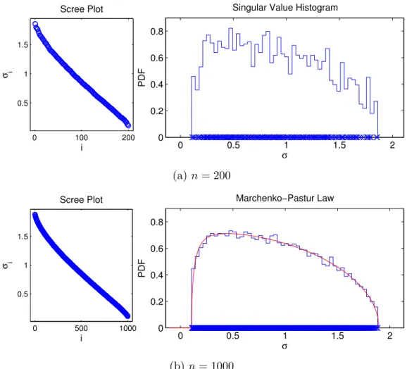
where a = τ(1−√c) and b = τ(1 +√c). Figure 2.1 shows the empirical singular value distributions of two i.i.d. random Gaussian matrices, one withn = 200 and the other with n = 1000. Clearly the empirical singular value distribution is converging to the Marcenko-Pastur law predicted by (2.10).

Figure 2.2 shows the singular value spectrum of a matrix Xe_n drawn from the model (2.5) withr= 3 and{θ1, θ2, θ3}={4, 3, 2}. The noiseXn is drawn from the Marcenko-Pastur law with τ = 1. In this case, one can show that the critical point is κ= 1. All three signals are above the critical point, so Theorem II.1 predicts that the leading 3 singular values ofXe_nwill separate from the bulk spectrum and converge asymptotically to the locationsρi =D−1µX(1/θ

2

i), fori= 1,2,3. Figure 2.2 corroborates this result. Conversely, Figure 2.3 shows a different realization of the same model where the third signal is nowθ3 = 0.95. In this case,θ3 < κ, so Theorem II.1 predicts

that _eσ3 will not separate from the bulk spectrum. Figure 2.3 again corroborates this

result.

Note that, although the theoretical results in this section are asymptotic in nature, Figures 2.1-2.3 demonstrate an important observation: random matrices of even mod-est sizes often closely follow their limiting behavior. This observation is important in practice. Indeed, it suggests that it is reasonable to design algorithms for matrix

(33)

0 100 200 0.5 1 1.5 Scree Plot i σ i 0 0.5 1 1.5 2 0 0.2 0.4 0.6 0.8 σ PDF

Singular Value Histogram

(a)n= 200 0 500 1000 0.5 1 1.5 Scree Plot i σ i 0 0.5 1 1.5 2 0 0.2 0.4 0.6 0.8 σ PDF Marchenko−Pastur Law (b)n= 1000

Figure 2.1: Singular values of acn×nmatrix with i.i.d. Gaussian entries for two values of n. Left: singular value scree plots. Right: empirical singular value historgrams. The red curve denotes the limiting Marcenko-Pastur law (2.10).

models that are based on asymptotic results, which can be expected to reasonably approximate the statistics of the empirical data. We now return to the problem of optimally estimating a low-rank matrix corrupted by random noise.

2.3 Optimal Low-Rank Matrix Estimation

Recall the low-rank plus noise model from (2.5):

e

Xn =Ln+Xn, (2.11)

where Ln = Pr

i=1θiuiviH is an unknown low-rank matrix of (known) rank r with singular valuesθi and singular vectors ui and vi, andXn is an additive noise matrix.

(34)

0 0.5 1 1.5 2 2.5 3 3.5 4 4.5 0 0.2 0.4 0.6 0.8 σ PDF Spiked Marchenko−Pastur

Figure 2.2: Singular value spectrum of Xe_n drawn from the model (2.5) with r = 3 and {θ1, θ2, θ3}={4, 3, 2}. The noise Xn is drawn from the Marcenko-Pastur law with τ = 1. The blue X’s denote the singular values of Xe_n, the blue curve denotes their empirical histogram, and the red curve is the limiting spectrum predicted by Theorem II.1. All three signals are above the critical point κ = 1, so the location of the extreme singular values are asymptotically given byρi =Dµ−1X(1/θ

2 i), fori= 1,2,3. 0 0.5 1 1.5 2 2.5 3 3.5 4 4.5 0 0.2 0.4 0.6 0.8 σ PDF Spiked Marchenko−Pastur

Figure 2.3: Singular value spectrum of Xe_n drawn from the model (2.5) with r = 3 and {θ1, θ2, θ3} ={4, 3, 0.95}. The noise Xn is drawn from the Marcenko-Pastur law withτ = 1. The blue X’s denote the singular values ofXe_n, the blue curve denotes their empirical histogram, and the red curve is the limiting spectrum predicted by Theorem II.1. The third signal θ3 = 0.95 is less than the critical point κ = 1, so it

does not separate from the bulk spectrum.

2.3.1 Oracle Denoising Problem

Suppose that we are interested in producing an estimate of Ln given an instance of Xe_n. One way to formulate this problem is the oracle denoising problem

w? = arg min [w1, ..., wr]T∈Rr r X i=1 θiuivHi − r X i=1 wieuiev H i F , (2.12)

(35)

where _eσi are the singular values and{eui,evi} are the singular vectors of Xen.

Problem (2.12) seeks the best approximation of the latent low-rank signal matrix

Ln by an optimally weighted combination of estimates of its left and right singular vectors. We refer to (2.12) as an oracle problem because it implicitly depends on the latent low-rank matrix Ln. Nonetheless, note that the TSVD of rank r and SVT are both feasible points for (2.12). Indeed, the truncated SVD corresponds to choosing weights wi = eσi1{i ≤ r} and SVT with parameter τ ≥ σer+1 corresponds to wi = (σei −τ)+. However, (2.12) can be solved in closed-form [26], yielding the expression w?_i = r X j=1 θj(eu H i uj)(ev H i vj), i= 1, . . . , r. (2.13) Of course, (2.13) cannot be computed in practice because it depends on the la-tent low-rank singular vectors ui and vi that we would like to estimate, but it gives insight into the properties of the optimal weights w?. Indeed, when u_ei and evi are good estimates of ui and vi, respectively, we expect eu

H

i ui and ev H

i vi to be close to 1. Consequently, from (2.13), we expect w?

i ≈ θi. Conversely, when eui and evi are poor estimates of ui and vi, respectively, we expect eu

H

i ui and viHevi to be closer to 0 and w?

i < θi. In other words, (2.13) shows that the optimal singular value shrinkage is inversely proportional to the accuracy of the estimated principal subspaces. As a special case, if θi → ∞, then clearlyue

H

i ui →1 and viHevi →1, so the optimal weights

w?_i must have the property that the absolute shrinkage vanishes as θi → ∞. This shows that, the SVT estimator, which applies a constant shrinkage to each singular value of its input, will necessarily produce suboptimal low-rank estimates in general. See [26] for more details.

Note that the constituent quantities {θj, ue H i uj, ev

H

i vj} of the solution (2.13) to (2.12) are exactly of the form analyzed in Section 2.2. Therefore, while we cannot compute (2.13) in practice, we can obtain asymptotic expressions for them in the large matrix limit whenXnis a suitable random matrix (e.g., an i.i.d. random matrix). The following theorem [26] formalizes this observation.

Theorem II.3. (Optimal Low-Rank Matrix Estimation [26]). Suppose that (Xn)ij

are i.i.d. random variables with zero-mean, variance σ2, and bounded higher order

moments, and suppose that θ1 > θ2 > . . . > θr > σ. Then, as m, n → ∞ such that

m/n→c∈(0,∞), we have that w_i?+ 2 DµXe (_eσi) D0 µ e X(eσi) a.s. −→0 for i= 1, . . . , r, (2.14)

(36)

where µ_X_e(t) = 1 q−r q X i=r+1 δ(t−_eσi), (2.15)

with q = min(m, n) is the empirical singular value density of Xe_n and D_µ

e

X is the

D-transform (2.7) of the measure µ_X_e.

Theorem II.3 establishes that the weightsw?_i—the solution to the oracle denoising problem (2.12)—converge in the large matrix limit to a certain non-random integral transformation of the limiting noise distribution µ

e

X. 2.3.2 Data-Driven OptShrink Estimator

In practice, Theorem II.3 suggests the following data-driven OptShrink estimator [26], defined for a given matrix Y ∈_Cm×n _{and rank} _r _as

OptShrink_r(Y) = r X i=1 −2 DµY(σi) D0 µY(σi) uiviH, (2.16)

where Y =UΣVH _{is the SVD of} _Y _{with singular values} _σ i and µY(t) = 1 q−r q X i=r+1 δ(t−σi) (2.17)

is the empirical mass function of the noise-only singular values of Y with q = min(m, n). Equation 2.16 approximates the optimal shrinkage from Theorem II.3 by plugging in the empirical distribution of the noise-only (non-leading) singular val-ues, µY, in place of the limiting distribution, µX, to which the empirical distribution is converging. By Theorem II.3, OptShrink_r(Xe) asymptotically solves the oracle denoising problem (2.12).

OptShrink has a single parameter r ∈ _N that directly specifies the rank of its output matrix. Rather than applying a constant shrinkage to each singular value of the input matrix as in SVT, the OptShrink estimator partitions the singular values of its input matrix into signals {σ1, . . . , σr} and noise {σr+1, . . . , σq} and uses the empirical mass function of the noise singular values to estimate the optimal (nonlinear, in general) shrinkage (2.14) to apply to each signal singular value. See [26, 27] for additional detail and intuition.

(37)

2.3.3 Computational Cost

The computational cost of OptShrink is the cost of computing a full SVD2 _plus

the O(r(m+n)) computations required to compute the D-transform terms in (2.16), which reduce to summations for the choice of µY in (2.17).

2_{In practice, one need only compute the singular values} _σ

1, . . . , σq and the leading r singular

(38)

CHAPTER III

Improved Robust PCA Using Optimal

Data-Driven Singular Value Shrinkage

3.1 Introduction

Principal component analysis (PCA) is a powerful technique for uncovering latent low-rank structure in high dimensional datasets. It is ubiquitous in statistical signal processing theory and practice and is the first step in many inferential procedures for detection, estimation and classification. It is well-known, however, that PCA is brittle in the sense that relatively few outliers can severely degrade the quality of low-rank components estimated from noisy data. This, in turn, degrades the performance of inferential tasks that utilize these estimated low-rank components. Robust PCA aims to mitigate such problems by producing the best (with respect to squared error) low-rank estimates that are robust to outlier contamination.

Recent breakthroughs [1, 31–33] have established that one can reliably recover a low-rank matrix in the presence of outliers by solving a convex optimization problem of the form

min

L,S kLk?+λkSk1 s.t. Y =L+S,

(3.1)

where Y is the observed data matrix, kLk? is the the nuclear norm (sum of singular values) of the low-rank component L, and kSk1 is the elementwise `1 norm of the

sparse component S. Indeed, sufficient conditions on L and S are given in [31, 32] to guarantee that the solution to (3.1) will exactly recover the low-rank and sparse components of the noiseless modelY =L+S. However, much less is known about the noisy setting—whenY is also corrupted by dense noise—except the unsurprising fact that one cannot expect error-free recovery. There is no theoretical reason to expect that a convex optimization-based model like (3.1) that was designed for the noiseless

(39)

setting will also be optimal in the noisy setting.

In [26] it is shown that, in the noisy but outlier-free setting, the low-rank compo-nents produced by solving any convex optimization problem are provably suboptimal. Indeed, [26] shows that the OptShrink estimator (described in Chapter II of this the-sis) provably outperforms convex optimization-based methods for low-rank matrix denoising. In this chapter, our goal is to apply these insights from low-rank matrix estimation in the context of performing robust PCA on noisy data.

3.1.1 Contributions

We first motivate the need for robust PCA algorithms by providing a first-principles analysis of the effect of outliers on the singular vectors of a noisy low-rank plus sparse matrix. Our analysis demonstrates that PCA is robust to noise but highly sensitive to even relatively few outliers in the data matrix. We then propose a new alternating minimization algorithm for robust PCA that uses the OptShrink estimator to improve the quality of the estimated low-rank component. Our proposed method is suitable for application in any inverse problem setting. Unlike existing methods, our algorithm does not correspond to a convex objective; however, we observe that it behaves well in practice. In particular, we demonstrate that our proposed method outperforms con-ventional robust PCA methods both in terms of quantitative reconstruction accuracy and qualitative interpretability of the components for two diverse applications: back-ground subtraction and dynamic magnetic resonance imaging (MRI) reconstruction from highly undersampled measurements.

3.1.2 Organization

This chapter is organized as follows. In Section 3.2, we formulate our robust PCA problem, and, in Section 3.3, we analytically characterize the effect of outliers on the singular vectors of the observed matrix. We describe the conventional convex optimization-based approach to robust PCA in Section 3.4, and we propose an im-proved algorithm in Section 3.5. In Section 3.6, we provide numerical experiments that demonstrate the promising performance of our method compared to existing robust PCA methods. Finally, we summarize our findings in Section 3.7.

(40)

3.2 Problem Formulation

Consider the setting where anm×nobserved signal-plus-noise-plus-outliers matrix

Y is modeled as Y = r X i=1 θiuiviH | {z } =:L +S+X, (3.2)

where, without loss of generality, we assumem≤n. In (3.2),L represents the rank-r

low-rank signal matrix that we are interested in reliably recovering, where ui and vi are the left and right singular vectors associated with singular value θi. The matrix

S is modeled as Sij =    Qij with probability ps 0 with probability 1−ps,

where Qij are elements drawn from an unknown distribution q with zero-mean, vari-anceσ2

q, and bounded higher order moments. The matrixSrepresents a sparse matrix of outliers (relative to L). We assume that the outlier probability ps logn/n to avoid any pathologies related to the sparsity pattern ofS interfering with the singular vectors of Y [34]. The matrixX has elements that are independently and identically distributed with zero mean, variance σ2_/n_{, and bounded higher order moments. In}

(3.2), we assume the outliers are sparse with respect to the standard Euclidean basis. If they are sparse with respect to some other basis (e.g., Fourier or wavelet), we can, without loss of generality, assume that (3.2) holds after an appropriate sparsifying transformation has been applied to the vectorized elements of the observed matrix.

3.3 Motivation for Robust PCA

Our goal is to estimate, as accurately as possible, the low-rank componentLfrom the matrix Y under the model (3.2). This objective is complicated by the presence of the outlier matrix S. Indeed, let

Y = m X i=1 e σieuiev H i (3.3)

be the SVD of Y. The following theorem extends results from random matrix theory [27] to quantify the degradation incurred when estimating the singular vectors of L