Robust mixture regression model fitting by Laplace distribution

(1)

ROBUST MIXTURE REGRESSION MODEL FITTING BY

LAPLACE DISTRIBUTION

by

YANRU XING

B.Eng., Tianjin Polytechnic University, China, 2002

LL.B., China University of Political Science and Law, China, 2005

A REPORT

submitted in partial fulﬁllment of the

requirements for the degree

MASTER OF SCIENCE

Department of Statistics

College of Arts and Sciences

KANSAS STATE UNIVERSITY

Manhattan, Kansas

2013

Approved by:

Major Professor

Weixing Song

(2)

Copyright

Yanru Xing

(3)

Abstract

A robust estimation procedure for mixture linear regression models is proposed in this

report by assuming the error terms follow a Laplace distribution. EM algorithm is

imple-mented to conduct the estimation procedure of missing information based on the fact that

the Laplace distribution is a scale mixture of normal and a latent distribution. Finite sample

performance of the proposed algorithm is evaluated by some extensive simulation studies,

together with the comparisons made with other existing procedures in this literature. A

sensitivity study is also conducted based on a real data example to illustrate the application

of the proposed method.

Key words and phrases:

Least Absolute Deviation; EM Algorithm; Mixture Regression

Model; Normal Mixture; Laplace Distribution

(4)

List of Figures

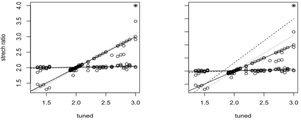
3.1 Figure 3.1 . . .

24 3.2 Figure 3.2 . . .

25 3.3 Figure 3.3 . . .

26

(6)

List of Tables

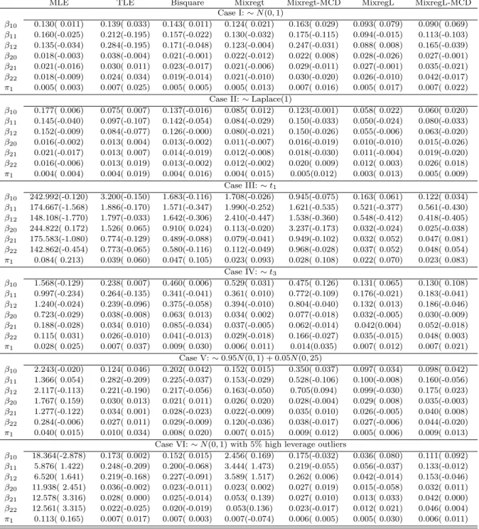
3.1 MSE(Bias) of Point Estimates for n = 100 . . . 21

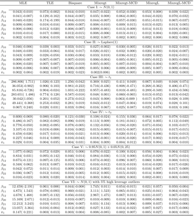
3.2 MSE(Bias) of Point Estimates for n = 200 . . . 22

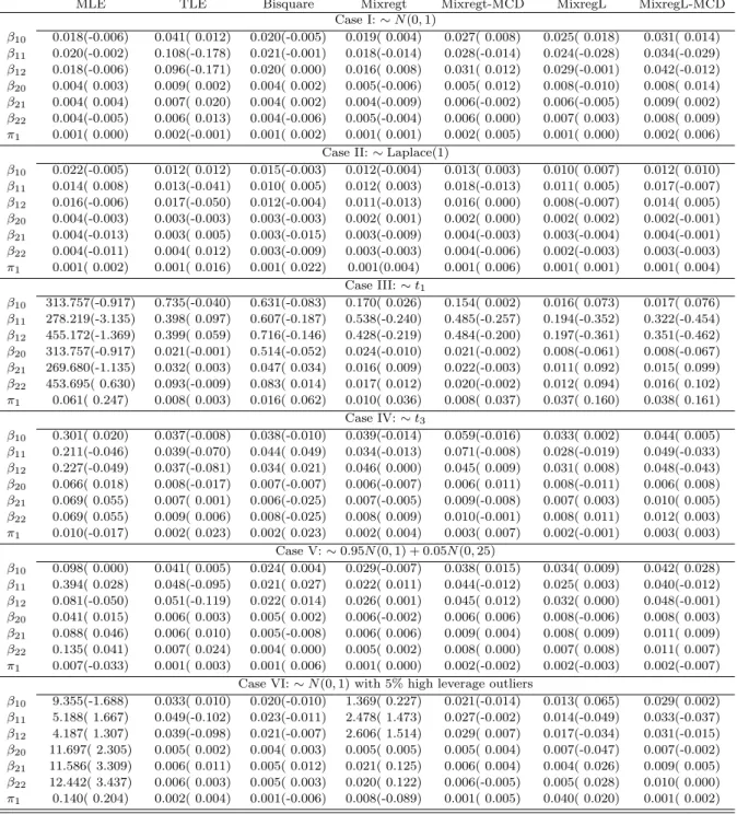
3.3 MSE(Bias) of Point Estimates for n = 400 . . . 23

(7)

Acknowledgments

I would like to express my deepest appreciation to Professor Weixing Song, who

continually and convincingly conveyed the spirit of insistence and creation in regard to

research. His exciting attitude in regard to teaching makes him be born for an instructor.

Without his guidance and persistent help, this report would not have been possible.

I also would like to thank Professor Kun Chen for his enthusiastic encouragement and

valuble critiques. I am grateful for Professor Weixin Yao's assistance and guidance. I obtain

most of the theoretical knowledge of Statistics by taking Professor Yao's classes.

Especially, I appreciate Professor Yao's contribution to part of the programming in the

simulation study.

I extend my sincere gratitude to Dr. Guihua Bai for providing me a GRA position.

Finally, I wish to thank my husband Huitao Liu for his support and encouragement

throughout my study.

(8)

Chapter 1 Introduction

Finite mixture models have been applied widely in practical and theoretical area over the

years because of its tractability. It can model complex distributions depending on the

choice of its appropriate components. Finite mixtures of distributions have constructed the

mathematical-based method to model various random phenomena; therefore, many science

ﬁelds adopt this kind of model to analysis data set, such as, biology, genetics, economics,

physical, medicine, social sciences, and so on. Over 100 years ago, famous biometrician Karl

Pearson (1894) used mixture models to analyzed the data set of measurements on the ratio

of forehead to body length of n=1000 crabs which were sampled from the Bay of Naples. The

mixture model was composed with two normal probability density functions with diﬀerent

means and variances in certain proportion respectively. He applied the method of moments

to ﬁt this mixture model and obtained his moments-based estimates of the ﬁve parameters.

Least absolute deviation (LAD) regression has been widely used in practice if robust

es-timates are desired. The research on its computation and theoretical properties is abundant

in the literature. A detailed survey on this topic can be found in Deilman (1984, 2005). In

this report, LAD will be applied to a class of mixture linear regression models to obtain

robust estimates of the regression coeﬃcients.

Wei (2012) proposed a robust estimation procedure for the mixture linear regression

models based on t distribution by extending McLachlan and Peel (2000)

s

work. The

re-search conducted in this report deals with the same questions as in Wei (2012), but with

(9)

the LAD technique, the Laplace distribution, instead of t-distribution, is used for achieving

robustness. In addition, the implementation of Wei (2012) procedure needs to specify the

degrees of freedom in the t-distribution, however, the laplace distribution does not need

to do the step of tuning parameters. Moreover, the natural connection between the LAD

procedure and the MLE procedure based on Laplace error makes the proposed procedure

more appealing.

1.1 Mixture Model Deﬁnition

Let

Y

1

,

. . .

,

Y

n

denote a random sample of size

n

from

g

components and suppose that the

mixture density

f

(

y

j

;

θ

) of

Y

j

can be expressed as following,

f

(

y

j

;

θ

) =

g

i=1

π

i

f

i

(

y

j

;

λ

i

)

,

(1.1)

where

π

i

is the weight or proportion of the

i

th

component, 0

≤

π

i

≤

1(

i

= 1

, . . . , g

), and

g

i=1

π

i

= 1.

θ

= (

π

1

, . . . , π

g

, λ

1

, . . . , λ

i

) is the set of unknown parameters and

λ

i

denote the

parameter vector of the density function

f

i

(

y

j

;

λ

i

). The

f

i

(

y

j

;

λ

i

) is the density function of

the

i

th

component. Let

z

j

be a categorical random variable over from 1 to

g

with probabilities

π

1

, . . . , π

g

, respectively.

1.2 Maximum Likelihood Estimation and EM

Algo-rithm

Maximum likelihood (ML) is the most commonly used approach to the ﬁtting of mixture

model. The estimate ˆ

θ

is obtained by an appropriate solution of the likelihood equation in

regular situation,

∂L

(

θ

)

(10)

The likelihood function of

θ

in model (1.1) is formed by the sample size

n

and given by

L

(

θ

;

y

) =

n

j=1

(

g

i=1

π

i

f

i

(

y

j

;

λ

i

))

.

(1.2)

It is equivalent to maximize the log likelihood function when we want to maximize the

likelihood function and the log likelihood function is suggested as

log

L

(

θ

;

y

) = log(

n

j=1

(

g

i=1

π

i

f

i

(

y

j

;

λ

i

)))

(1.3)

=

n

j=1

log(

g

i=1

π

i

f

i

(

y

j

;

λ

i

))

.

The ML estimate of parameters

θ

can be described as

ˆ

θ

= arg max

n

j=1

log(

g

i=1

π

i

f

i

(

y

j

;

λ

i

))

.

(1.4)

Hence, the solution of the following equation is the ML estimate of

θ

,

∂

log

L

(

θ

;

y

)

∂θ

= 0

.

It is obvious that the above equation does not have explicit solutions unless in trivial case.

However, the solutions of the likelihood equation can be obtained by the application of EM

algorithm (Dempster et al., 1977).

EM algorithm is a very useful method to handle the incomplete-Data problem. In the

procedure of ﬁtting parametric mixture model with EM algorithm, the observed data vector

y

= (

y

1

, . . . , y

n

)

T

is viewed as being incomplete as the associated component-label vectors,

z

= (

z

1

, . . . , z

n

)

T

, are not observable. Since each

y

j

come from one of the

g

components in

the mixture model,

z

j

is a

g

-dimensional vector where

z

ij

= (

z

j

)

i

= 1 or 0 depending on

whether

y

j

arise from the

i

th

component of the mixture model or not. The complete-data

vector is

(11)

The complete Log likelihood log

L

c

(

θ

;

y, z

) for complete-data vector

y

c

is given by

log

L

c

(

θ

;

y, z

) = log

n

j=1

(

g

i=1

(

π

i

f

i

(

y

j

;

λ

i

))

zij

)

(1.5)

=

n

j=1 g

i=1

z

ij

log(

π

i

f

i

(

y

j

;

λ

i

))

=

g

i=1 n

j=1

z

ij

(log

π

i

+ log

f

i

(

y

j

;

λ

i

))

.

The EM algorithm proceeds iteratively in two steps, E-step (expectation step) and

M-step (maximization M-step). E-M-step handles the unobservable data, which compute the

con-ditional expectation of complete log likelihood given observable vector

y

and using initial

parameter set

θ

(0)

_for

_θ

_{. The M-step on the (}

_k

_{+ 1)}

th

_{iteration maximize the expectation in}

the E-step with respect to

θ

and obtain the updated estimates

θ

(k+1)

_{. The EM algorithm}

(iterative procedure) can be summarized as:

1. Input initial values

θ

(0)

_{= (}

_π

(0) 1

, . . . , π

(0)

g

, λ

(0)₁

, . . . , λ

(0)g

) for the parameters.

2. E-step: For the (

k

+ 1)

th

iteration, compute

Q

(

θ, θ

(k)

) =

E

(log

L

c

(

θ

;

y, z

)

|

y, θ

(k)

)

(1.6)

=

E

(

n

j=1 g

i=1

z

ij

log(

π

i

f

i

(

y

i

;

λ

i

))

|

y, θ

(k)

)

=

n

j=1 g

i=1

E

(

z

ij

|

y, θ

(k)

) log (

π

i

f

i

(

y

j

;

λ

i

))

.

When compute the expectation of log

L

c

(

θ

;

y, z

), we only need to compute the

expecta-tion of

z

ij

given

y

and

θ

(k)

,

E

(

z

ij

|

y, θ

(k)

) =

τ

ij(k+1)

=

π

(k) i

f

i

(

y

j

;

λ

(ik)

)

g i=1

π

(k) i

f

i

(

y

j

;

λ

(ik)

)

.

(1.7)

3. M-step: compute the estimate of

θ

which maximizes

Q

(

θ, θ

(k)

_),

(12)

4. The E-step and M-step are repeated until certain criterion is satisﬁed.

1.3 Normal Mixture

Pearson (1894)’s experiment suggests that the normal mixture model is useful in ﬁtting the

data which have asymmetrical distributions. We use the normal mixture as an example to

conduct EM algorithm. The component normal density has mean

μ

i

and covariance

σ

i2

and

the mixture density function is given by

f

(

y

;

θ

) =

g

i=1

π

i

f

i

(

y

;

λ

i

) =

g

i=1

π

i

φ

i

(

y

;

μ

i

, σ

i2

) =

g

i=1

π

i

√

2 πσ

i

e

−(y−2σμi2_i)2

_.

_(1.8)

The EM algorithm for normal mixture model is showed as

1. Input initial values for parameters:

π

_i(0)

,

μ

(0)_i

, and

σ

_i2(0)

.

2. E-step: Compute the expectation of the complete log likelihood given

θ

(k)

_and

obser-vation

y

at the (

k

+ 1)

th

iteration. The procedure is the following:

Q

(

θ, θ

(k)

) =

E

(log

L

c

(

θ

;

y, z

)

|

y, θ

(k)

) =

n

j=1 g

i=1

E

(

z

ij

|

y, θ

(k)

) log (

π

i

f

i

(

y

j

;

λ

i

))

.

(1.9)

Let

τ

_ij(k+1)

=

τ

i

(

y

j

;

θ

(k)

) =

E

(

z

ij

|

y, θ

(k)

), then

Q

(

θ, θ

(k)

) =

n

j=1 g

i=1

τ

ij

log

π

i

−

1

2

n

j=1 g

i=1

τ

ij

log 2

πσ

i2

−

1

2

n

j=1 g

i=1

τ

ij

(

y

j

−

μ

i

)

2

σ

2 i

,

(1.10)

τ

(k+1) ij

=

π

(k) i

φ

i

(

y

j

;

μ

(ik)

, σ

2( k) i

)

g i=1

π

(k) i

φ

i

(

y

j

;

μ

i(k)

, σ

i2(k)

)

.

(1.11)

3. M-step: Take the derivative of

Q

(

θ, θ

(k)

_{) with respect to}

_θ

_{, we obtain}

π

(k+1) i

=

n

j=1

τ

(k+1) ij

/n,

(1.12)

μ

(k+1) i

=

n j=1

τ

(k+1) ij

y

j

n j=1

τ

(k+1) ij

,

(1.13)

σ

2(k+1) i

=

n j=1

τ

(k+1) ij

(

y

j

−

μ

(ik+1)

)

2

n j=1

τ

(k+1) ij

.

(1.14)

(13)

1.4 Mixture of Normal Linear Regression Models

Linear regression model has been studied and applied widely in the analysis of statistical

relations between variables. In practice, the data in a data set may originate from diﬀerent

normal population. Hence the mixture of normal linear regression models is very useful to

solve the practical problems in many ﬁelds, like marketing, biology, agriculture, economics,

and so on.

Let

Z

be a latent class variable and deﬁne

Z

=

i

(

i

= 1

,

2 , . . . , g

)

. Y

is the scalar response

variable which depends on the

p

-dimensional predictor

X

, and their relations could be

constructed by the following linear regression model:

Y

=

X

β

i

+

ε

i

, i

= 1

,

2 , . . . , g,

where

β

i

= (

β

i1

,

. . .

,

β

ip

)

,

ε

i

and

X

are independent. The density of

ε

i

follows normal

distribution

f

i

(

· ) with mean 0 and variance

σ

2i

. Suppose

P

(

Z

=

i

) =

π

i

, then the conditional

density of

Y

given

X

without observing

Z

is,

f

(

y

|

x, θ

) =

g

i=1

π

i

f

i

(

y

;

x

β

i

, σ

i2

)

,

(1.15)

where

θ

= (

π

1

, β

1

, σ

21

, . . . , π

g

, β

g

, σ

2g

)

.

Perform the procedures of EM algorithm as in section 1.3 for

f

(

y

|

x, θ

).

1. Take initial value

θ

(0)

_{= (}

_π

(0)

1

, . . . , π

(0) g

, β

1(0)

, . . . , β

(0) g

, σ

12(0)

, . . . , σ

2(0) g

)

.

2. E-step: For the (

k

+1)

th

iteration, compute the conditional expectation of the complete

log likelihood,

E

[

Z

ij

|

y, θ

(k)

] =

τ

ij(k+1)

=

π

(k) i

f

i

(

y

j

;

x

j

β

( k) i

, σ

2( k) i

)

g i=1

π

(k) i

f

i

(

y

j

;

x

j

β

i(k)

, σ

i2(k)

)

,

(1.16)

where

f

i

(

y

j

;

x

j

β

i(k)

, σ

2( k) i

) =

1 σ

(k) i

√

2 π

e

−(yj−xj β(ik))2 2σ_i2(k)

_.

_(1.17)

3. M-step: Update the value of parameters depending on

θ

(k)

_.

π

(k+1) i

=

n

j=1

τ

(k+1) ij

n

,

(1.18)

(14)

β

(k+1) i

= arg min

n

j=1

τ

(k+1) ij

(

y

j

−

x

j

β

i

)(

y

j

−

x

j

β

i

)

= (

n

j=1

τ

(k+1) ij

x

j

x

j

)

−1 n

j=1

τ

(k+1) ij

x

j

y

j

,

(1.19)

σ

2(k+1) i

=

n j=1

τ

(k+1) ij

(

y

j

−

x

j

β

i(k+1)

)

2

n j=1

τ

(k+1) ij

.

(1.20)

(15)

Chapter 2 EM Algorithm for Robust Mixture

Regression

2.1 Laplace Distribution

Let

X

be a p-dimensional vector of explanatory variables, and

Y

be a scalar response

variable. We use a linear regression model to investigate the relationship between

Y

and

X

. For the mixture linear regression setup, we assume that (

X

, Y

) come from one of the

following

g

≥

2 linear regression models with probability

π

i

,

i

= 1, 2,

. . .

,

g

,

Y

=

X

β

i

+

σ

i

ε

i

, i

= 1

,

2 , . . . , g,

(2.1)

where

g_i₌₁

π

i

= 1,

β

i

’s are unknown

p

-dimensional vectors of regression coeﬃcients,

σ

i

’s

are unknown positive scalars. The random error

ε

i

’s are assumed to be independent of

X

i

’s.

It is commonly assumed that the density functions of

ε

i

’s are members in a location-scale

family with mean 0 and variances 1. In this report the design variable

X

is assumed to be

random, but the proposed estimation procedure also works for the ﬁxed design.

If

g

= 1, LAD estimate of

β

is the minimizer of the target function

Q

(

β

) =

n_j₌₁

|

Y

j

−

X

j

β

|

, where (

X

j

, Y

j

)

n_j₌₁

is a sample from model (2.1). However, if

g >

1, the formulation of

LAD target function is not straightforward since for a sample, we simply do not know which

regression model an observation arises from. Our formulation of the LAD target function

is motivated by the fact that the maximum likelihood estimate of the regression coeﬃcients

(16)

given double exponentially distributed random error is indeed the LAD estimator for

g

= 1.

Therefore, for

g

≥

2 case, we assume that

ε

i

follows a double exponential distribution with

location 0 and scale parameter 1

/

√

2, which makes the variance of

ε

i

being 1,

i

= 1

,

2 , . . . , g

.

Then it is easily seen that for a sample

S

=

{

(

X

_j

, Y

j

)

, j

= 1

,

2 , . . . , n

}

from the model (2.1),

the log likelihood function of

θ

= (

β

1

, σ

12

, π

1

, β

2

, σ

22

, π

2

, . . . , β

g

, σ

g2

, π

g

) can be written as

log

L

(

θ

;

S

) =

n

j=1

log

g

i=1

π

i

√

2 σ

i

exp

(

−

√

2 |

Y

j

−

X

j

β

i

|

σ

i

)

.

(2.2)

Thus the maximum likelihood estimate of

θ

can be obtained by maximizing log

L

(

θ

;

S

)

with respect to

θ

. Usually no explicit solution can be obtained, and some numerical method

will be needed.

For the case

g

= 1, many algorithms are developed in the literature to tackle the

mini-mization problem ˆ

β

= arg min

Q

(

β

), such as the linear programming, least angle regression,

the modiﬁed maximum likelihood method by Li and Arce (2004), and others. An often

adopted but ad-hoc scheme for ﬁnding the solution

β

is to directly take the derivative of

Q

(

β

) with respect to

β

, and set it equal to 0. Here

σ

2

_{is treated as a nuisance parameter.}

By doing this, we obtain

∂Q

(

β

)

∂β

=

−

n

j=1

X

j

sgn

(

Y

j

−

X

j

β

) = 0

,

(2.3)

where

sgn

(

· ) is the sign function which takes -1, 0, 1 if the argument is negative, 0

and positive, respectively.

Let

w

j

= 1

/

|

Y

j

−

X

j

β

|

, and rewrite the equation (2.3) as

n

j=1

w

j

X

j

(

Y

j

−

X

j

β

) = 0. Thus by supplying an initial value

β

0

for

β

, the updated

value

β

can be found by the weighted least square solution

β

1

= (

n

j=1

w

j

X

j

X

j

)

−1 n

j=1

w

j

X

j

Y

j

.

(2.4)

By iterating the above procedure, one can eventually ﬁnd an approximate solution to

arg min

θ

Q

(

θ

).

(17)

stated above and an EM algorithm in conjunction with the Laplace distribution is found in

Phillips (2002). For the sake of completeness, we brieﬂy describe the procedure of Phillip

(2002) here.

Andrews and Mallows (1974) showed that a Laplace distribution in fact can be expressed

as a mixture of a normal distribution and another distribution related to exponential

dis-tribution. To be speciﬁc, supposed

Z

and

V

be two random variables,

V

has a distribution

with density function

v

−3

_exp

₍

₋

₍₂

_v

2

₎

−1

_),

_{v >}

_{0, and given}

_V

₌

_v

_{, the conditional}

distribu-tion of

Z

is normal with mean 0 and variance

σ

2

_/

₍₂

_v

2

_{). The joint density function}

_f

₍

_{z, v}

₎

of

Z

and

V

can be written as

f

(

z, v

) =

√

v

πσ

exp

(

−

v

2

_z

2

σ

2

)

1 v

3

exp

(

−

1

2 v

2

)

.

(2.5)

Hence,

Z

marginally has a Laplace distribution with density function

h

ε

(

z

) =

exp

(

−

√

2 |

z

|

/σ

)

/

(

√

2 σ

). Based on this ﬁnding, Phillips (2002) developed an EM algorithm to search for the

minimizer of

Q

(

β

).

Considering

V

as a latent variable, if

V

could be observed, then the complete

log-Likelihood function of

θ

= (

β, σ

2

_{), based on the sample}

_P

_{= (}

_X

j

, Y

j

, V

j

)

n_j₌₁

, is

log

L

(

θ

;

P

) =

−

n

2 log

πσ

2

₋

1 σ

2 n

j=1

V

2 j

(

Y

j

−

X

j

β

)

2

−

n

j=1

log

V

_j2

−

1

2

n

j=1

1 V

2 j

.

(2.6)

Following the two steps in EM algorithm procedure, assume that

θ

(k)

_{= (}

_β

(k)

_{, σ}

2(k)

_{) is the}

value in the

k

th

iteration, then in the (

k

+ 1)

th

iteration, we have to compute the conditional

expectation of the complete log likelihood function log

L

(

θ

;

P

) ﬁrst, given the observed data

set (

Y

j

, X

j

)

n_j₌₁

and

θ

=

θ

(k)

, the procedure is showed as

E

[log

L

(

θ

;

P

)

|

S

] =

−

n

2 log

πσ

2

₋

n j=1

E

[

V

j2

|

θ

( k)

_,

₍

_X

j

, Y

j

)

n_j₌₁

](

Y

j

−

X

j

β

)

2

σ

2

−

n

j=1

E

[log

V

_j2

|

θ

(k)

,

(

X

j

, X

j

)

n_j₌₁

]

−

1

2

n

j=1

E

[

1 V

2 j

|

θ

(k)

_,

₍

_X

j

, Y

j

)

n_j₌₁

]

.

(18)

For the next step, maximize the conditional complete log likelihood expectation with

respect to

θ

. Denote

w

j

=

E

[

V

j2

|

θ

(k)

,

(

X

j

, Y

j

)

n₍j=1)

], and we notice that the third and fourth

terms on the right hand side of the above function do not involve the unknown

regres-sion parameters, such that maximizing the above conditional expectation is equivalent to

maximizing the following terms with respect to

θ

,

−

n

2 log

σ

2

₋

n j=1

w

j

(

Y

j

−

X

j

β

)

2

σ

2

.

Phillips (2002) showed

w

j

=

E

[

V

j2

|

θ

(k)

,

(

X

j

, Y

j

)

n_j₌₁

] =

σ

(k)

/

(

√

2 |

Y

j

−

X

j

β

(k)

|

), this implies

that the solution of

β

(k+1)

_{indeed is the same as the one based on (2.4). It is also easy to}

see that

σ

2(k+1)

_{can be estimated by}

_σ

2(k+1)

_{= 2}

n

j=1

w

j

(

Y

j

−

X

j

β

(k+1)

₎

2

_/n

_{. The above}

methodology will be extended to mixture regression setting.

2.2 Mixture Model with Laplace Distribution

In model (2.1), assume that

ε

i

’s follow a Laplace distribution with mean 0 and scale

param-eter 1/

√

2. For

i

= 1

,

2 , . . . , g, j

= 1

,

2 , . . . , n,

denote

Z

ij

as latent Bernoulli variables such

that

Z

ij

=

1 if

j

th observation (

X

j

, Y

j

) is from

i

th component;

0 otherwise.

If the full data set

T

=

{

(

X

j

, Y

j

, Z

ij

)

}

_i₌₁_,₂_,...,g_;_j₌₁_,₂_,...,n

are observable, then the complete

log likelihood function of

θ

= (

β

1

, σ

21

, π

1

, β

2

, σ

22

, π

2

, . . . , β

g

, σ

g2

, π

g

) can be written as

log

L

(

θ

;

T

) =

n

j=1 g

i=1

Z

ij

log

√

π

i

2 σ

i

exp

(

−

√

2 |

Y

j

−

X

j

β

i

|

σ

i

)

.

(2.7)

From Andrews and Mallows (1974) mentioned above, we know that a Laplace distributed

random variable is a scale mixture of a normal random variable and another variable

re-lated to exponential distribution. Denote

V

j

, coupled with (

X

j

, Y

j

), as the latent scale

variable,

j

= 1

,

2 , . . . , n

, then the complete log likelihood function of

θ

, based on

D

=

(19)

{

X

j

, Y

j

, V

j

, Z

ij

}

_i₌₁_,₂_,...,g_;_j₌₁_,₂_,...,n

, has the form

log

L

(

θ

;

D

) =

n

j=1 g

i=1

Z

ij

log

π

i

√

V

j

πσ

i

exp

(

−

V

2 j

(

Y

j

−

X

j

β

i

)

2

σ

2 i

)

1 V

3 j

exp

(

−

1

2 V

2 j

)

(2.8)

=

n

j=1 g

i=1

Z

ij

log

π

i

−

1

2

n

j=1 g

i=1

Z

ij

log

πσ

2i

−

n

j=1 g

i=1

Z

ij

V

2 j

(

Y

j

−

X

j

β

i

)

2

σ

2 i

−

n

j=1 g

i=1

Z

ij

log

V

j2

−

1

2

n

j=1 g

i=1

Z

ij

V

2 j

.

Based on EM algorithm principle, for the E-step, we have to calculate the conditional

expectation

E

[

L

(

θ

;

D

)

|

S, θ

(0)

_{], where}

_θ

(0)

_{= (}

_β

(0) 1

, σ

2(0) 1

, π

(0) 1

, . . . , β

(0) g

, σ

g2(0)

, π

(0)g

) is a proper

initial value for

θ

and

S

=

{

(

X

j

, Y

j

)

}

nj=1

. Since the last two terms in (2.8) do not involve

the unknown regression parameters, we can simply drop them from the analysis. Thus, to

ﬁnd

E

[

L

(

θ

;

D

)

|

S, θ

(0)

_{], we only need to calculate the following two terms}

τ

ij

=

E

[

Z

ij

|

S, θ

(0)

]

,

δ

ij

=

E

[

V

j2

|

S, θ

(0)

, Z

ij

= 1]

.

(2.9)

Refer to section 1.3, we obtain

τ

(1) ij

=

π

(0) i

σ

i−1(0)

exp

(

−

√

2 |

Y

j

−

X

j

β

i(0)

|

/σ

i(0)

)

g m=1

π

(0) m

σ

m−1(0)

exp

(

−

√

2 |

Y

j

−

X

j

β

m(0)

|

/σ

(0)m

)

.

(2.10)

Follow the same thread as in Phillips (2002) to compute

δ

ij

δ

(1) ij

=

σ

(0) i

√

2 |

Y

j

−

X

j

β

i(0)

|

.

(2.11)

In the M-step, the following expression will be maximized with respect to

π

i

’s,

β

i

’s, and

σ

2 i

’s,

n

j=1 g

i=1

τ

ij

log

π

i

−

1

2

n

j=1 g

i=1

τ

ij

log

σ

i2

−

n

j=1 g

i=1

τ

ij

δ

ij

(

Y

j

−

X

j

β

i

)

2

σ

2 i

.

(2.12)

(20)

2.3 EM Algorithm

We propose the following EM algorithm to maximize function (2.12).

1. Choose an initial value for

θ

= (

β

1

, σ

12

, π

i

, . . . , β

g

, σ

g2

, π

g

).

2. E-Step: at the (

k

+ 1)

th

iteration, calculate

τ

_ij(k+1)

and

δ

_ij(k+1)

from equation (2.10) and

(2.11) with (0) replaced by (

k

).

3. M-Step: at the (

k

+ 1)th iteration, use the following formulas to calculate the

maxi-mizer of (2.12):

π

(k+1) i

=

1 n

n

j=1

τ

(k+1) ij

,

(2.13)

β

(k+1) i

= (

n

j=1

τ

(k+1) ij

δ

(ijk+1)

X

j

X

j

)

−1

(

n

j=1

τ

(k+1) ij

δ

ij(k+1)

X

j

Y

j

)

,

(2.14)

and

σ

2(k+1) i

=

2

n_j₌₁

τ

_ij(k+1)

δ

_ij(k+1)

(

Y

j

−

X

j

β

i(k+1)

)

2

n j=1

τ

(k+1) ij

.

(2.15)

4. Repeat steps 2 and 3 until the convergence is obtained.

If we further assume that all

σ

2

i

are equal, then in the above EM algorithm, a common

initial value for

σ

2

i

should be used, and

σ

2

can be updated in M-Step by

σ

2(k+1)

₌

2

n j=1

g i=1

τ

(k+1) ij

δ

( k+1) ij

(

Y

j

−

X

j

β

i(k+1)

)

2

n

.

(2.16)

The robustness of the above EM procedure follows from the adoption of LAD regression.

It is also obvious from the formulae of the updated

β

i

’s in each iteration. Note that the

factor reciprocally related to the term

|

Y

j

−

X

j

β

i(k)

|

, meaning that larger residuals give smaller

values of

δ

(_ijk+1)

, hence, down-weight the corresponding observations when calculating the

estimates.

It is easy to see that when updating

β

_i(k+1)

, the weight

δ

ij

can be simpliﬁed to

δ

ij

=

1 /

|

Y

j

−

X

j

β

i(k)

|

. After updating

β

(

k+1)

(21)

in one population case, we can update

σ

i

using formula

σ

(k+1) i

=

√

2

n_j₌₁

τ

_ij(k+1)

δ

_ij(k+1)

|

Y

j

−

X

j

β

i(k+1)

|

n j=1

τ

(k+1) ij

.

(2.17)

Accordingly, when all

σ

2

i

´s are assumed to be equal, then one can update the common

variance by

σ

(k+1)

₌

√

2

n_j₌₁

g_i₌₁

τ

_ij(k+1)

δ

_ij(k+1)

|

Y

j

−

X

j

β

i(k+1)

|

n

.

(2.18)

The EM algorithm proposed above for calculating the estimate of

β

indeed is an iterated

reweighted least square (IRLS) procedure, as the one proposed in Schlossmacher (1973) for

one population case and the weights are given by

τ

_ij(k+1)

δ

_ij(k+1)

in the (

k

+ 1)

th

iteration.

Extra attention should be paid when programming the proposed EM algorithm. In the case

of

g

= 1, Schlossmacher (1973) warned that if a perfect LAD ﬁt occurs, i.e.,

Y

j

−

X

j

β

ˆ

i

= 0

for some

i, j

and ˆ

β

i

, then the algorithm will eventually gives

Y

j

−

X

j

β

ik

≈

0 when iteration

proceeds. As a result,

δ

(_ijk+1)

which is reciprocally related to

|

Y

j

−

X

j

β

ik

|

will be very large,

and numerical instability would follow. Although Phillips (2002) noticed that this problem

rarely arises in the case of

g

= 1, this does occur often in our case, which is not out of

expectation, simply because more than one regression models provide more chance for a

perfect LAD ﬁtting. But simply adopting Schlossmacher (1973)’s weight scheme by setting

δ

(k+1)

ij

= 0 whenever

|

Y

j

−

X

j

β

ik

|

< e

for a pre-assigned

e >

0 is not quite reasonable. It makes

much sense to allocate big weights for small residuals and small weights for big residuals.

A cogent argument on this issue is provided in Phillips (2002). In our simulation study, we

simply adopt a hard threshold rule to control the extremely small LAD residuals in each

iteration step. Under this rule,

δ

_ij(k+1)

will be assigned a value of 10

6

_{for any perfect LAD ﬁt.}

We also tried other threshold values, such as 10

8

_{, 10}

10

_{in the simulation, all these choices}

generate almost identical results. For the sake of brevity, we only report the simulation

results by using 10

6

_{as the threshold value.}

It is well known that in IRLS procedure, numerical instability could occur if the weights

are very small. A common way to deal with this issue is to impose a hard threshold on

τ

_ij(k+1)

(22)

obtained in the (

k

+ 1)

th

iteration. Namely, for a pre-speciﬁed value

e

say, if

τ

_ij(k+1)

> e

, then

τ

(k+1)

ij

itself will be used for the next iteration; otherwise,

e

will be used as the weight for

the next iteration. Same technique is used in Wei (2012). In our simulation study,

e

= 10

−6

is adopted.

2.4 Trim high leverage points

Similar to the traditional M-estimate for linear regression and Wei (2012)’s mixture

re-gression by

t

-distribution, the above EM algorithm based on Laplace distribution is robust

against outliers along

y

-direction, but not in

x

-direction, which is also conﬁrmed by the

sensitivity study conducted in Chapter 3. As a consequence, if there are any high leverage

points in the data sets, then the proposed EM algorithm might not follow our expectation,

and certain modification would be necessary. An obvious modification is first to identify

these high leverage points, then just discard them.

A commonly used method is to calculate the leverage value for each observation using

the following formula,

h

jj

=

n

−1

+ (

n

−

1)

−1

MD

j

,

where

MD

j

= (

X

j

−

X

¯

)

S

−1

(

X

j

−

X

¯

), ¯

X, S

are the sample mean and sample covariance

matrix of

X

j

’s, respectively. The

j

th observation will be identiﬁed as a high leverage point

if

h

jj

>

2 p/n

, where

p

is the dimension of

X

. To avoid the masking eﬀect caused by using

¯

X

and

S

in detecting the high leverage points, like some high leverage points may inﬂuence

other high leverage points to be identiﬁed, some robust estimation of the population mean

and covariance matrix of

X

can be used instead of the sample mean and sample

covari-ance. Wei (2012) adopted the minimum covariance determinant (MCD) estimators for the

population mean and covariance matrix, which is implemented by the Fast MCD algorithm

developed in Rousseeuw and Van Driessen (1999). Certainly, other robust estimates of the

population mean and covariance matrix could be also used for this purpose, for example, the

Stahel-Donoho (SD) estimator from Stahel (1981) and Donoho (1982). The

j

th observation

(23)

will be considered as a high leverage point if the resulting

MD

j

exceeds the threshold

χ

2p,0.975

.

This threshold is proposed by Pison et al. (2002). In the simulation studies, we apply the

proposed EM algorithm based on Laplace distribution after removing the observations with

(24)

Chapter 3 Numerical Studies

In this chapter, an extensive simulation study will be conducted to assess the ﬁnite sample

performance of the proposed robust estimation procedure. It is well known that the label

switching is always an issue when evaluating diﬀerent estimation methods in mixture

mod-els, and there is no widely accepted labeling standard. In our simulation, similar to Wei

(2012), we simply choose the labels by minimizing the distance to the true parameter values.

The eﬀects of labeling schemes on comparison diﬀerent estimation procedures deserve an

independent research in the future.

3.1 Simulation Studies

In the simulation study, let all components have equal variance. The reason for doing this

is that, if the variances are not the same, the log-likelihood function (2.7) is unbounded and

goes to inﬁnity if one observation exactly lies on one component line and its corresponding

variance goes to 0, which makes the simulation very unstable.

To compare our proposed method with some existing estimation procedures, we generate

sample data (

X

j1

, X

j2

, Y

j

)

nj=1

from the following two-component mixture regression models

which are also used in Wei (2012):

Y

=

0 +

X

1

+

X

2

+

ε

1

,

if Z=1,

0 −

X

1

−

X

2

+

ε

2

,

if Z=2,

(25)

where

Z

indicates which component an observation comes from. That is, the data are

generated from a two-component mixture linear regression model with

β

1

= (

β

10

, β

11

, β

12

)

=

(0

,

1 ,

1)

and

β

2

= (

β

20

, β

21

, β

22

)

= (0

,

−

1 ,

−

1)

. The predictors

X

1

∼

N

(0

,

1) and

X

2

∼

N

(0

,

1) are independent. The random error

ε

1

and

ε

2

are also independent and have the

same distribution as

ε

. To check the eﬀects of diﬀerent distributions of

ε

and the high

leverage outliers in

x

-direction on various estimation methods, the following six cases are

considered:

Case I :

ε

∼

N

(0

,

1), standard normal distribution.

Case II:

ε

∼

Laplace distribution with mean 0 and variance 1.

Case III:

ε

∼

t

1,

t

-distribution with 1 degree of freedom or the Cauchy distribution.

Case IV:

ε

∼

t

3

,

t

-distribution with 3 degrees of freedom.

Case V:

ε

∼

0 .

95 N

(0

,

1) + 0

.

05 N

(0

,

25), a mixture with two normal distributions.

Case VI:

ε

∼

N

(0

,

1) with 5% high leverage outliers being

X

1

=

X

2

= 20 and

Y

= 100.

Case I is often used to evaluate the eﬃciency of diﬀerent estimation methods compared

to the traditional MLE when the error is exactly normally distributed and there are no

outliers. For Case II, the estimation methods proposed in this report will provide the MLE

of unknown parameters, which, as in the ﬁrst case, would serve a reference line to evaluate

the performance of other estimation procedures. Both Case III and IV are heavy tailed

distributions and often used in literature to mimic the outlier situations. Case V would

produce 5% data likely to be low leverage outliers, and in Case VI, 5% observations are

replicated serving as the high leverage outliers, which will be used to check the robustness

of estimation procedures against the high leverage outliers.

Seven estimation methods will be compared in the simulation study:

1. Maximum likelihood estimate based on normality assumption (MLE).

(26)

2. Trimmed likelihood estimator (TLE) proposed by Neykov et al. (2007).

3. Robust modiﬁed EM algorithm based on bisquare (Bisquare) proposed by Bai et al.

(2012).

4. Robust mixture regression based on

t

-distribution (Mixregt) proposed by Wei (2012).

5. Trimmed mixture regression based on

t

-distribution with MCD trimming method

(Mixregt-MCD).

6. The proposed robust EM mixture regression based on Laplace-distribution (MixregL).

7. Trimmed mixture regression based on Laplace-distribution with MCD trimming method

(MixregL-MCD).

In all simulation studies, the iteration is terminated whenever the diﬀerence of the

like-lihood functions from the current step and the previous step is less than 10

−6

_.

The simulation results are shown in the following tables (Table 1, 2, and 3), which report

the mean squared errors (MSE) and bias (Bias) of the parameter estimates for each case

in diﬀerent estimate methods. Sample sizes are 100, 200, and 400 for each case. From the

simulation studies, we can see that if the true distribution of

ε

is normal, the MSEs of MLE

procedure are slightly bigger than our proposed method for the ﬁrst regression component

when the sample size is 100, but MLE will show its superiority over all other methods when

the sample size gets bigger. For other cases when the distribution of

ε

has a heavier tail,

contaminated by some outliers, or there are high leverage outlier in the data set, then MLE

fails to provide reasonable estimates regardless of sample size.

TLE and Bisquare perform very well for all the cases where

ε

has a lighter tail, except

case III where

ε

has a

t

-distribution with 1 degree of freedom. The overall performance of

the Mixregt proposed by Wei (2012) is satisfying when sample size gets bigger except for

the Case VI when high leverage points present in the data set, but this disadvantage could

be remedied by the modiﬁed procedure Mixregt-MCD.

(27)

The simulation results also suggest that the proposed method in this report outperforms

or at least is comparable to any other methods. It is rather unexpected that our proposed

method performs better than the Mixregt and Mixregt-MCD procedures even when

ε

has

a

t

-distribution. The bigger MSEs in the latter two procedures might be resulted from the

extra step involved in the algorithm, the selection of

v

, which is the degrees of freedom of

the

t

-distribution.

MCD estimator is mentioned above, which is used in Mixregt-MCD and MixregL-MCD

to remove high leverage outliers. For case VI, Mixregt-MCD performs better than Mixregt,

but MixregL-MCD doesn’t show obvious improvment to MixregL in this simulation.

A common criticism about the EM algorithm is its slow convergence. This can also be

seen from our simulation study. The average numbers of iterations to achieve convergence

using the MixregL procedure are 96, 97, 78, 98, 102, and 10 for cases from I to VI,

respec-tively, when the sample size is 100; 110, 99, 65, 105, 117, 14 when the sample size is 200;

and 124, 111, 41, 123, 119, 17 when the sample size is 400. The number of iterations depend

on the choice of the stopping rule. For example, if the iteration is terminated whenever the

diﬀerence of the likelihood functions from the current step and the previouse step is less

than 10

−4

_{, then the average numbers of iterations to achieve convergence using the MixregL}

procedure are 62, 62, 36, 63, 64, 10 for cases from I to VI, respectively, when the sample

size is 100. Some accelerating methods might be used here to speed up the convergence,

but we shall not seek this possibility in the current report.

3.2 Real Data Example

In this section, a sensitivity study will be conducted which is based on a real data set to

compare how outliers aﬀect various diﬀerent estimation procedures. A typical real data

set suitable for mixture regression modeling is the tone data collected in a tone perception

experiment of Cohen (1984). In the experiment, a pure fundamental tone was played to

a trained musician and electronically generated overtones were added, determined by a

Robust mixture regression model fitting by Laplace distribution