Redundancy and Complexity Metrics for Big Data Classification: Towards Smart Data

(1)

Date of publication xxxx 00, 0000, date of current version xxxx 00, 0000. Digital Object Identifier 10.1109/ACCESS.2017.DOI

Redundancy and Complexity Metrics for

Big Data Classification: Towards Smart

Data

JESUS MAILLO1_{, ISAAC TRIGUERO}2_{, (Member, IEEE), and FRANCISCO HERRERA}1,3_, (Senior Member, IEEE)

1_{The Department of Computer Science and Artificial Intelligence, University of Granada, 18071 Granada, Spain}

2_{Computational Optimisation and Learning Lab (COL), School of Computer Science, University of Nottingham, Nottingham NG8 1BB, United Kingdom} 3

Faculty of Computing and Information Technology, King Abdulaziz University (KAU) Jeddah, Saudi Arabia Corresponding author: Jesus Maillo (e-mail: [email protected]).

ABSTRACT

It is recognized the importance of knowing the descriptive properties of a dataset when tackling a data science problem. Having information about the redundancy, complexity and density of a problem allows us to make decisions as to which data preprocessing and machine learning techniques are most suitable. In classification problems, there are multiple metrics to describe the overlapping of the features between classes, class imbalances or separability, among others. However, these metrics may not scale up well when dealing with big datasets, or may not simply be sufficiently informative in this context. In this paper, we provide a package of metrics for big data classification problems. In particular, we propose two new big data metrics: Neighborhood Density and Decision Tree Progression, which study density and accuracy progression by discarding half of the samples. In addition, we enable a number of basic metrics to handle big data. The experimental study carried out in standard big data classification problems shows that our metrics can quickly characterize big datasets. We identified a clear redundancy of information in most datasets, so that, discarding randomly 75% of the samples does not drastically affect the accuracy of the classifiers used. Thus, the proposed big data metrics, which are available as a Spark-Package, provide a fast assessment of the shape of a classification dataset prior to applying big data preprocessing, toward smart data.

INDEX TERMS Big Data, Smart Data, Classification, Redundancy, Complexity, Apache Spark

I. INTRODUCTION

In many different applications, we are collecting large amounts of data with the purpose of obtaining useful insights through a Knowledge Discovery in Databases process [1]. Their nature is very diverse, with implications for society in all its fields, such as theoretical physics in studies carried out at CERN [2], implications for politics [3], new challenges posed in social media [4] or advances in medical applications [5], among others.

Despite the ease of finding/gathering large amounts of data in a multitude of fields, this data needs to be preprocessed to discard those samples that are disruptive, and select the data that provides quality information for machine learning. This process, included in the denominated Smart Data technolo-gies [6], aims to obtain quality data [7] through the applica-tion of data preprocessing algorithms [8]. In [9], we discussed the use of the k Nearest Neighbors (kNN) algorithm [10] as

a key technique capable of imputing missing values [11] and reducing redundant [12] and noisy data [13] to obtain quality data from big datasets. In addition, there are contributions as proposed by Liu et al. [14], where the results are improved and the runtime reduced in classification problems by select-ing the appropriate classification rule accordselect-ing to a given neighborhood, instead of using the complete dataset. In [15], the authors deal with the large dissimilarity data by proposing an evidential clustering method that obtains good results with the random selection of part samples to decrease the runtime and space complexity.

The main assumption of most current research in big data is that having more data would enable better insights. However, having more data does not necessarily imply that we can obtain more relevant information, and may result in unnecessary computational cost. Smart data technologies alleviate this issue [9]. However, the application of very

(2)

so-phisticated big data preprocessing algorithms may also not be needed if, for example, we identify high levels of redundancy. With this hypothesis and the problem highlighted, we ask the following question:

• When is Big Data too much data for machine learning? To appropriately answer this question, we need to know the characteristics of the dataset to be addressed before applying any big data preprocessing or machine learning algorithm. In that way, we may avoid running time-consuming techniques without knowing if they are necessary. To achieve this, there are metrics that mainly measure three aspects: complexity [16], which is defined as the difficulty in classifying unseen samples; redundancy [17] that refers to the existence of in-stances where the information they provide is already present in other instances; and density [18] which represents a high number of instances in relation to the domain of the problem. These metrics are commonly used in the field of auto machine learning [19] as extracted features from a dataset, which help determine the best pipelines (i.e. combination of preprocessing and learning algorithms) for a new given dataset [20]. However, existing metrics were developed for standard problems [21], quality measures present problems of computational scalability in order to tackle big datasets. These problems come from their design, for example: density metrics based on the pruning of completely connected graphs [22], or complexity metrics based non-linearity of classifier based on sequential classification algorithms [23], both with very high computational complexity.

In this paper, we postulate that the big data literature is often neglecting the fact that there is redundancy in the data. Collect and store data for the sake of it may cause data storage and computational problems. Therefore, it is necessary to characterize a problem by means of complexity, redundancy and density metrics prior to applying big data preprocessing or machine learning algorithms.

We propose two new big data metrics to measure den-sity and complexity, called Neighborhood Denden-sity (ND) and Decision Tree Progression (DTP) respectively, to detect the redundancy of information in big datasets and reduce their size when necessary, alleviating the issues mentioned above.

The main contributions of this paper are: A) We proposed two new big data metrics:

• ND presents the proximity of samples by calculating the percentual difference of the Euclidean distance, which is calculated with all available data, and with the half of them randomly chosen.

• DTP measures complexity and redundancy by train-ing two decision trees with the totality of the data, and discarding half of them randomly. The percentual difference of the accuracy obtained with each model is calculated to reflect the loss of information. Moreover, we implement some of the best-known met-rics in the literature [21] re-designed for execution in big datasets. An open source Spark-based [24] package has been developed that includes the two proposed

metrics and a set of literature metrics, which is available on the spark-packages platform: https://spark-packages. org/package/JMailloH/ComplexityMetrics

B) Redundancy has been analized.An experimental study has been carried out composed of ND and DTP, as well as literature metrics adapted to the big data environment and three classification algorithms. In addition, a ran-dom data subsampling analyis has been carried out at different levels to investigate the effect of the sample size.

The remainder of this paper is organized as follows. Section II introduces state-of-the-art on scalable complexity metrics selected for experimental study. Then, Section III de-tails the two proposed metrics and analyze their complexity. Section IV and Section V describe the experimental setup and multiple analyses of results, respectively. Finally, Section VI outlines the conclusions and future work.

II. COMPLEXITY MEASURES

This section provides insights about the complexity metrics existing in the literature that have been selected to be devel-oped in Spark. Thus, these metrics can be calculated over large datasets. Lorena et al. [21] perform an extensive review of existing metrics in the literature to study the complexity of problems.

For the definition of metrics, we consider a dataset T formed by nsamples. Each sample is composed of (x, y), where the input variables is described as an array x = [x1, ..., xm], also named in the document as features. The

output variableyis composed byncclasses.

A. F1. MAXIMUM FISHER’S DISCRIMINANT RATIO This metric measures the overlap between the features of the different classes of the problem. Specifically, it calculates the overlap of each feature separately, and takes the highest.

Orriols puig et al. [25] propose different equations for the F1 metric, differentiating continuous or ordinal features. However, for the development of this publication we selected the proposal of Mollineda et al. [26] which deals with binary problems (classification problems composed of two classes) and multiclass problems. F1 is calculated for each feature separately, and finally the most restrictive of all is returned:

F1=maxm

i=1 rfi (1)

rfiis computed as defined Equation 2.

rfi= Pnc j=1ncj(µ fi cj −µ fi₎2 Pnc j=1 Pncj l=1(x j li−µ fi cj)2 (2)

Wherencj is the number of instances of the classj,µ fi cj is

the average of thei-th feature of the samples of the classj, µfi _{is the average of the}_i_{-th feature of all instances and}_xj

li

is the specific value of thei-th feature for a particular sample x.

(3)

The F1 is a complexity metric with a reduced computa-tional cost, and this makes it of high interest for big data prob-lems. However, it only studies overlapping domains between instances of different classes, considering single feature. This decreases the quality of the extracted information.

Its computational complexity is O(m · n). The metric domain is[0,+∞], and it is inversely proportional, meaning that if the resulting value is high, the complexity of the problem will be low.

B. F2. VOLUME OF OVERLAPPING REGION

The F2 metric calculates the overlap between the samples of the different classes. In this case, it considers the domain (maximum and minimum values) of all features. For this reason, it is called “Volume” of overlapping region. Cummins [27] proposes the metric defined in Equation 3.

F2=

m

Y

i

max{0,minmax(fi)−maxmin(fi)}

maxmax(fi)−minmin(fi)

(3) Letfiandcjbe thei-th feature and thej-th class

respec-tively, where:

· minmax(fi) =min(max(fic1),max(f c2

i ). . .max(f cj i ))

· minmin(fi) =min(min(fic1),min(f c2

i ). . .min(f cj i ))

· maxmax(fi) =max(max(fic1),max(f c2

i ). . .max(f cj i ))

· maxmin(fi) =max(min(fic1),min(f c2

i ). . .min(f cj i ))

Although it has a computational cost higher than F1, it represents a more realistic simulation of the operation of the classifiers because it considers multiple features. However, it does not count the number of affected instances in the overlapping area, it only considers the overlapping domain.

Its computational complexity isO(m·n·nc)and its domain

is[0,1]. It is directly proportional, therefore, a value 1 in the metric means a high complexity.

C. F3. MAXIMUM INDIVIDUAL FEATURE EFFICIENCY The basis of this complexity metrics is to account for whether classes are linearly separable by a single feature [25]. To do this, it calculates the ratio of examples that are not in the overlap area and the total number of examples:

F3=maxm_i₌₁n−no(fi)

n (4)

Where no(fi) is the number of samples found in the

overlap area, whose membership is defined by Equation 5.

no(fi) = n

X

j=1

I(xji>maxmin(fi)∧xji<minmax(fi))

(5) I returns value 1 if the condition is satisfied, and 0 if the condition is unsatisfied. Thus, it counts the number of samples in the overlap area.

With the equations presented, the efficiency of each feature is defined as the fraction of all remaining instances separable

by the mentioned feature. Thus, the highest separability ob-tained by a single feature is counted. F3 is a restrictive com-plexity metric, because it considers its separability by only one feature. Data mining algorithms extract knowledge and patterns related to all features and the relationship between them.

The F3 metric addresses the major disadvantage of the F1 and F2 metrics by counting the number of samples affected. However, similar to F1, it only considers a single feature.

Its computational complexity is O(m · n ·nc), with a

domain of[0,1]. The metric is inversely proportional to the complexity.

D. F4. COLLECTIVE FEATURE EFFICIENCY

The F4 metric [25] is a natural extension of the F3 metric, which adds a more restrictive component by considering all features. The process of calculating the metric consists of the following three iterative steps:

1) F3 is computed to determine which feature is the most discriminatory.

2) The instances that are outside the overlap area corre-sponding to the feature selected in step 1 are discarded. 3) The feature selected in step 1 is removed, and the

procedure is repeated until all features are considered. It is formally described in Equation 6.

F4= n−no(fmax(Tl))

n (6)

Considering that the setTi is subject to the changes

de-scribed in the iterative procedure,fmax(Ti)is:

fmax(Ti) ={fj|maxjm=1n−no(fj))} (7)

The F4 metric is the most appropriate in the literature for studying the complexity of a classification problem. It counts the number of samples affected, and also considers all features in an iterative process. As a disadvantage, it is the slowest of the proposed metrics because of its counting and iteration process.

Its computational complexity is higher than F3, because it iterates on all features O(m2_·_n_·_n

c). In the same way as

F3, complexity is inversely proportional to the value of the metric, and its domain is[0,1].

E. C1. ENTROPY OF CLASS PROPORTIONS

Lorena et al. [28] proposes an entropy-based metric to mea-sure the imbalance between classes [29]. The mathematical expression is presented in Equation 8.

C1=− 1 log(nc) nc X i=1 pilog(pi) (8)

Wherepirepresents the proportion of instances of the class

i(pi=ni/n).

It has a computational complexity ofO(n). The metric do-main is[0,1]and is inversely proportional to the complexity.

(4)

A value of 1 indicates a perfect balance between the number of instances of the different classes.

F. C2. IMBALANCE RATIO

It is the most widely used metric in the literature to measure class imbalance in classification problems. The selected ap-proach is proposed by Tanwani et al. [30] to handle multiclass problem. The Equation 9 presents the mathematical expres-sion to calculate C2. C2=nc−1 nc nc X i=1 ni n−ni (9) C2 is an important metric for the information it provides and its fast calculation. Classifiers significantly reduce the quality of their results when fed with imbalanced datasets [31], knowing about the imbalance ratio allows the correct application of preprocessing techniques to balance the num-ber of class instances. Thus improve the results obtained by classifiers.

Its computational complexity is O(n), and the metric domain is[1,+∞]. The relationship between the metric and the complexity of the problem is directly proportional, so a value of 1 indicates a perfect balance between classes.

III. BIG DATA METRICS: NEIGHBORHOOD DENSITY AND DECISION TREE PROGRESSION

This section presents the two proposed metrics specifically designed to deal with big datasets. Section III-A motivates the design and development of the two proposed metrics. Neighborhood Density (Section III-B) takes as its basis the distance between samples and how discarding half of the samples affects it. Decision Tree Progression (Section III-C) shows the progression of the accuracy obtained by Decision Tree with all instances and dropping half of them. Finally, it summarizes the implemented metrics (Section III-D) that compose the open source packageComplexityMetrics.

A. MOTIVATION

To the best of our knowledge, there are no specific metrics for big data problems in the literature. The design and creation of complexity and density metrics capable of providing valuable information and scaling up to big datasets is an underde-veloped area. From this necessity, we designed two specific metrics with the nearest neighbors (1NN) and DT algorithms to study density and complexity respectively.

The ND metric is based on the 1NN algorithm, using the Euclidean distance as a measure of similarity. By discarding instances, the distance increases and the percentage differ-ence determines the density. The 1NN algorithm is used because using larger values for the number of neighbors would dilute the information provided by the metric. The main goal of this metric is to compute the churn in density of the dataset when removing randomly a subset of instances. To do this, we calculate the average distance between instances. If we use k>1 the probability of using the same instances to

compute the average distance among instances will increase, and therefore the metric would lose information. The DTP metric is based on the Decision Tree classifier. Decision Tree was selected because of its high scalability in both the training and classification stages, to quickly characterize the problem. Using accuracy as a metric, the percentage difference is calculated by randomly discarding half of the instances. Any classifier that satisfies these characteristics can be replaced to have a complexity metric based on a classifier with a different behavior.

In order to propose density and complexity metrics for big data problems, percentage values have been prefixed in terms of the number of instances involved. Thus, a balance is obtained between runtime and a quality representation of the density and complexity of the dataset. These values are the following: 10% validation and 90% training, as well as a random sub-sampling of 50%. In addition, using very high or low percentages may lead the metric to extreme situations. This is why we suggest those values.

B. ND. NEIGHBORHOOD DENSITY

In this subsection, we present an original proposal for esti-mating density loss in a dataset based on neighborhood. For the design of the ND metric, we based on the hypothesis that the distance ratio represents the density of the dataset. However, simply the distance between the samples is not enough information, as it varies depending on the dataset without implying a higher or lower density. In order to pro-vide valuable information, we will calculate the variation of the mean distance between the samples of a dataset, counting the whole dataset, and reducing it by half.

To do this, the mean distance between all instances is calculated, considering the nearest neighbor. Afterwards, half of the samples are randomly drawn, and the procedure is repeated to obtain the mean distance again. The percentage increase of the distance will be the value that indicates the density.

Figure 1 and Algorithm 1 describe the workflow for calcu-lating the ND metric, which is explained below:

1) We start from the complete dataset, and split it into 2, leaving 90% of the data in a set that we will call neighborhood and the remaining 10% in one that will be named validation.

2) The average distance of all instances of thevalidation

set is calculated, along to theneighborhoodset. The dis-tance is calculated as performed by the 1NN algorithm. The average distance obtained will then be namedd. 3) It takes half of the instances of theneighborhoodset and

calculates again the average distance of all the instances

fromvalidationset. The average distance obtained will

be namedds.

4) Once calculateddandds, the result of the metric will be

the percentage difference of the distances. Equation 10 presents the mathematical expression performed.

(5)

Neighborhood KNN-IS distance ҧ 𝑑 KNN-IS distance 𝑑𝑠 50% 𝑠𝑢𝑏𝑠𝑎𝑚𝑝𝑙𝑒 Validation Dataset 90% 𝑠𝑢𝑏𝑠𝑎𝑚𝑝𝑙𝑒 10% 𝑠𝑢𝑏𝑠𝑎𝑚𝑝𝑙𝑒

FIGURE 1:Neighborhood Density Workflow

Algorithm 1Neighborhood Density Require: data

1: neighborhood, validation←randomSplit(data,90%,10%) 2: neighborhoodsub←sample(50%)

3:

4: d←averageDistance(neighborhood, validation) 5: ds←averageDistance(neighborhoodsub, validation)

6: return (d−ds/d)·100

ND= d−ds

d ·100 (10)

Going deeper at the technical level, the development of the ND metric code uses the kNN-IS algorithm [32] to calculate 1NN, KNN-IS algorithm gets the exact nearest neighbors, implemented on the Spark platform.

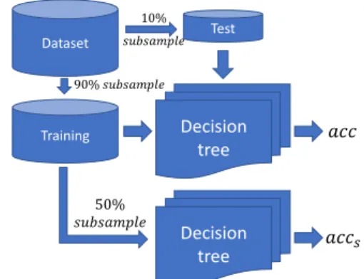
C. DTP. DECISION TREE PROGRESSION

In this section, we detail the second original proposal for estimating accuracy loss in a dataset with the decision tree algorithm. In this occasion, for the design of the DTP metric, we take the accuracy of the decision tree classifier as a measure of complexity. However, accuracy by itself does not enable us to know how complexity evolves with respect to the number of instances of the dataset. To obtain valuable information, we calculate the accuracy loss by excluding half of the instances in the training.

To do this, a small sample is taken to be used as a test set and then a DT is trained with the complete set and half of the data. Accuracy is calculated with the two trained models by classifying the same test set. The metric consists of the percentage difference between the accuracy. If it returns a negative value, it implies that you have obtained a better result with the model trained with half of the data.

The metric workflow is presented in Figure 2 and the Algorithm 2, which is composed of the following steps:

1) We start from the complete dataset, and split it into 2, leaving 90% of the data in a set that we will calltraining

and the remaining 10% in one that will receive the name oftest. Training Decision tree 𝑎𝑐𝑐 Decision tree 𝑎𝑐𝑐𝑠 50% 𝑠𝑢𝑏𝑠𝑎𝑚𝑝𝑙𝑒 Test Dataset 90% 𝑠𝑢𝑏𝑠𝑎𝑚𝑝𝑙𝑒 10% 𝑠𝑢𝑏𝑠𝑎𝑚𝑝𝑙𝑒

FIGURE 2:Decision Tree Progression Workflow

Algorithm 2Decision Tree Progression Require: data

1: training, test←randomSplit(data,90%,10%) 2: trainingsub←sample(50%)

3:

4: acc←accuracyDT(training, test) 5: accs←accuracyDT(trainingsub, test)

6: return (acc−accs/acc)·100

2) Afterwards, the DT is trained with the training set, and the test set is classified, calculating the accuracy (acc). 3) One-half of the instances of the training set are

dis-carded, and will be calledtraining_sub. We train a new DT withtrainingsubset, and classify thetestset,

keep-ing the accuracy (accs).

4) Once calculated acc and accs, we calculate the accuracy

percentage difference, following the Equation 11. DTP= acc−accs

acc ·100 (11)

The DT code used is the one available in the MLLib library. Its parameters are: Gini as impurity measure. Max-imum depth equal to 20 and maxMax-imum number of samples per bins set to 32.

D. SOFTWARE PACKAGE: COMPLEXITY METRICS All metrics presented in this paper are as a free software package ComplexityMetrics hosted in the spark-packages [33] library available at: https://spark-packages.org/package/ JMailloH/ComplexityMetrics.

The metrics have been developed under the Map Reduce paradigm [34] providing them with scalability to address large datasets. Specifically, the Apache Spark framework [24] has been selected due to its popularity and results against other distributed proposals [35]. In particular, the literature metrics have been implemented using the official machine learning library, MLlib [36], specifically with the Statistics class. The Statistics class calculates in a very efficient way the maximum, minimum and average values of each feature of the complete dataset. With these statistical values, the mathematical expressions for each metric described in the Section II are computed, obtaining the overlap by filtering

(6)

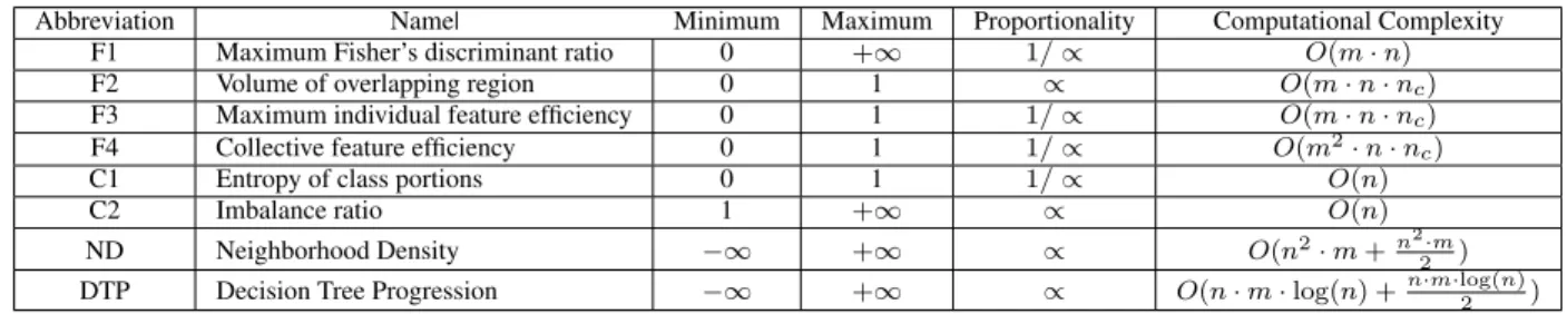
TABLE 1:Summary of the metrics

Abbreviation Name| Minimum Maximum Proportionality Computational Complexity

F1 Maximum Fisher’s discriminant ratio 0 +∞ 1/∝ O(m·n)

F2 Volume of overlapping region 0 1 ∝ O(m·n·nc)

F3 Maximum individual feature efficiency 0 1 1/∝ O(m·n·nc)

F4 Collective feature efficiency 0 1 1/∝ O(m2_·_n_·_nc₎

C1 Entropy of class portions 0 1 1/∝ O(n)

C2 Imbalance ratio 1 +∞ ∝ O(n)

ND Neighborhood Density −∞ +∞ ∝ O(n2_·_m₊n2·m

2 )

DTP Decision Tree Progression −∞ +∞ ∝ O(n·m·log(n) +n·m·log(₂ n))

the instances when it is necessary. The technical details of the original proposals have already been described in the Sections III-B and III-C.

Table 3 summarizes the abbreviation and name of each metric, indicating also the minimum and maximum value they can take, whether the complexity is directly or inversely proportional (∝ and 1/ ∝, respectively) to the value of the metric (Column Proportionality), and the computational complexity.

The computational complexity indicated is the sequential execution one. All implementations have been adapted to be executed in a distributed way using Spark’s primitive operations, providing high scalability to all of them.

IV. EXPERIMENTAL SET-UP

This section presents the details of the experimental set-up. It describes the datasets used (Section IV-B), the classification algorithms used and their parameters (Section IV-C), and fi-nally, the hardware and software characteristics under which the experimentation has been carried out (Section IV-A).

A. SOFTWARE AND HARDWARE SPECIFICATION The experiments have been executed in a cluster dedicated to distributed computing. The cluster is composed of a master node, and 14 compute nodes. Regarding software configura-tion: Spark (version 2.2.1), Scala (version 2.11.6) and HDFS (Version 2.6.0-cdh5.8.0) on the CentOS operating system (version 6.5).

The hardware performance of each machine is as follows: two Intel Xeon CPU E5-2620 processors (2 GHz), with 12 threads each (6 cores), 64 GB main memory and 15 MB cache memory. The connection between the machines is Infiniband at 40 Gb/s speed. With this configuration, the cluster can host a total of 256 map operations in parallel.

B. DATASETS

The experimental study consists of 6 standard big classi-fication datasets extracted from the UCI repository [37]. They have been selected for their high relevance in previous experimental studies in the field of big data classification. Table 2 summarizes the number of samples, features, and classes for each dataset.

For the experimentation carried out, a 5 fold cross-validation scheme was followed, with 80% dedicated to training and 20% to testing. In addition, the experimentation

TABLE 2:Description of the datasets Dataset #Samples #Features #Classes

Higgs 11,000,000 28 2 Ht_sensor 928,991 11 3 Skin 245,057 3 2 Susy 5,000,000 18 2 Watch_acc 3,540,962 20 7 Watch_gyr 3,205,431 20 7

TABLE 3:Instances for each dataset version

Dataset #Instances #Instances Training

Test 100% 75% 50% 25% Higgs 2,200,000 8,800,000 6,600,000 4,400,000 2,200,000 Ht_sensor 185,798 743,193 557,395 371,596 185,798 Skin 49,011 196,046 147,034 98,023 49,011 Susy 1,000,000 4,000,000 3,000,000 2,000,000 1,000,000 Watch_acc 708,192 2,832,770 2,124,577 1,416,385 708,192 Watch_gyr 641,086 2,564,345 1,923,259 1,282,172 641,086

has the particularity of making versions of each dataset by random subsampling, this technique is typically known as random undersampling (RUS) [38]. RUS is used in problems of class imbalance, to reduce the number of samples of the majority class and facilitate the learning of the classification algorithm used later. However, our objective is different, we want to know if we need all the samples or if they contain redundant information. Thus, following the cross validation scheme, on the one hand, RUS is applied to the training parti-tion maintaining the same proporparti-tion of classes. On the other hand, RUS is not applied to the test partition, allowing to compare the accuracy results between the different classifiers and different sub-sampling levels performed. Table 3 shows the number of instances in the test and train partitions for each applied subsampling level.

C. CLASSIFIERS AND PARAMETERS

All metrics described in Section II have been used for exper-imentation. In addition, in order to cover a larger behavior in the experimental study, we have used three classification algorithms with different characteristics. These three algo-rithms are developed for Big Data problems, and represent three families of algorithms: based on instances or similarity, entropy and weight optimization. The algorithms used and their parameters are listed below:

• Local Hybrid Spill tree Fuzzy k Nearest Neighbors (LHS-FkNN) [39]1: This algorithm is based on similar-ity, namely the Euclidean distance. The parameter used 1_{https://spark-packages.org/package/saurfang/spark-knn}

(7)

is k = 7, both in the class membership degree stage and the classification stage.

• Decision Tree (DT)2: This classifier is based on entropy and information gain. In the experiment carried out, it has been used a maximum depth of 20 and a maximum number of samples per leaf equal to 32. Gini impurity measure how often a randomly instance of the dataset is wrongly classified if it will be randomly labeled according to the distribution of labels of the dataset. • Multilayer Perceptron (MLP)3 _{: classifier based on}

weight adjustment, is a type of artificial feedforward neural network. For this experiment, we have used 2 hidden layers of 10 and 5 neurons, respectively. With a block size of 1000 and the maximum number of iterations equal to 500.

In Map Reduce-like implementations, it is also important to know the number of map tasks used. In all cases, 256 map operations have been used, which coincide with the maximum available in the cluster.

As we are dealing with standard classification problems, the accuracy metric was used to measure the quality of the results of the three classification algorithms used. The accu-racy is calculated by dividing the number of well-classified samples by the number of total samples.

V. ANALYSIS OF RESULTS

In this section, we study the results obtained by the classifi-cation algorithms and the metrics developed (Section V-A), its implications with data redundancy (Section V-B) and the scalability through the runtime (Section V-C).

A. METRICS AND ACCURACY ANALYSIS

The study is designed to analyze the importance of the quality and quantity of the data available in a big data problem. Specifically, a sub-sampling study is performed at 75%, 50% and 25% to analyze whether a large amount of available data is necessary, or the dataset contains redundant information.

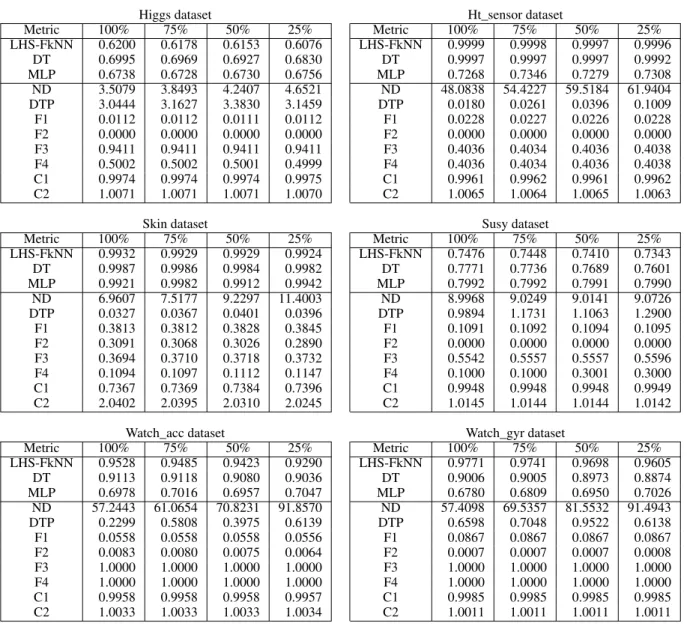
Table 4 show for the three classifiers used and each one of the metrics, the value obtained with the complete set (100%), and with the subsamples made, keeping 75%, 50% and 25% of the samples.

According to the results obtained, we can present the following conclusions:

• Focusing on the ND metric, there is an incremental pro-gression from 100% of the samples as they are discarded in blocks of 25%. This shows how dropping instances also reduces the density of the dataset. Reducing the density in the dataset leads to a lack of representation in the problem, and consequently, to an increase in its com-plexity. However, if we compare the density obtained with the complete dataset, and the density with 25%, the difference presented is very small. This shows us that we can discard instances without drastically affecting the 2_{https://spark.apache.org/docs/2.2.1/ml-classification-regression.html#decision-tree-classifier}

3_{https://spark.apache.org/docs/2.2.1/ml-classification-regression.html#multilayer-perceptron-classifier}

density obtained. To ensure this behavior, we can see the slight decrease in accuracy in the classifiers used, even slightly increasing with MLP.

• If we consider the DTP metric, it always keeps under 1 except for the Higgs dataset, up to 3. These low values represent the low loss of accuracy involved in discarding half of the dataset while training the DT classifier. In fact, if we compare DTP with 100% versus 25%, the differences are minimal. This information shows us that by discarding 75% of the instances, there is a minimal difference in the percentage loss of accuracy with re-spect to having all the instances.

• The accuracy of the classification algorithms does not drastically change even when 75% of the samples are drop randomly, which shows a clear redundancy of information. Going deeper into the analysis, we see how LHS-FkNN and DT are affected more by density loss. In the case of LHS-FkNN it is because it bases its learning on similarity, specifically on the Euclidean distance, thus defining the boundaries between classes. DT bases its learning on entropy, and specifically on the value taken by each node of the tree when deciding which class it belongs to. However, MLP learns by adjusting the weights of each neuron. For this reason, accuracy is maintained at similar values, improving slightly its results if we compare having 100% of the samples versus taking 25%.

• The F1 metric remains stable despite discarding in-stances. This shows how discarding instances does not affect the complexity of the problem. In addition, if we support the results of F1 with the accuracy obtained, it consolidates the existence of redundancy, and how discarding instances does not significantly harm the classifiers, improving the results for the MLP algorithm. • C1 and C2 metrics, related to the problem of class imbalance, measure the entropy of classes and the ratio of imbalance respectively. Both show the almost per-fect balance of all the datasets, except Skin, where C2 indicates us that there are double as many instances of one class with respect to the other. These metrics alone do not provide all the information desired to address a big data problem, and therefore require new metrics specific to large datasets. Joining several metrics gets useful information. An example would be the following: we have a dataset with C2 greater than 1, with DTP and ND with low values. This presents a high density and redundancy of information, with a moderate com-plexity. Thus, it would be more appropriate to apply sub-sampling techniques (such as instance selection or random undersampling) to reduce the size of the dataset as opposed to applying over-sampling techniques (such as prototype generation or random oversampling). • Finally, to highlight a weakness detected in the metrics

F2, F3 and F4, that belonging to the state-of-the-art in non-big data classification problems. The information they provide is contrary to that reflected by the

(8)

accu-TABLE 4:Progression of results with each subsampling

Higgs dataset Ht_sensor dataset

Metric 100% 75% 50% 25% Metric 100% 75% 50% 25% LHS-FkNN 0.6200 0.6178 0.6153 0.6076 LHS-FkNN 0.9999 0.9998 0.9997 0.9996 DT 0.6995 0.6969 0.6927 0.6830 DT 0.9997 0.9997 0.9997 0.9992 MLP 0.6738 0.6728 0.6730 0.6756 MLP 0.7268 0.7346 0.7279 0.7308 ND 3.5079 3.8493 4.2407 4.6521 ND 48.0838 54.4227 59.5184 61.9404 DTP 3.0444 3.1627 3.3830 3.1459 DTP 0.0180 0.0261 0.0396 0.1009 F1 0.0112 0.0112 0.0111 0.0112 F1 0.0228 0.0227 0.0226 0.0228 F2 0.0000 0.0000 0.0000 0.0000 F2 0.0000 0.0000 0.0000 0.0000 F3 0.9411 0.9411 0.9411 0.9411 F3 0.4036 0.4034 0.4036 0.4038 F4 0.5002 0.5002 0.5001 0.4999 F4 0.4036 0.4034 0.4036 0.4038 C1 0.9974 0.9974 0.9974 0.9975 C1 0.9961 0.9962 0.9961 0.9962 C2 1.0071 1.0071 1.0071 1.0070 C2 1.0065 1.0064 1.0065 1.0063

Skin dataset Susy dataset

Watch_acc dataset Watch_gyr dataset

racy reported by the classifiers, generating interest and relevance to the proposed metrics.

B. REDUNDANCY ANALYSIS

Once all metrics have been analyzed, we are ready to answer the question raised:

When is Big Data too much data for machine learning? Much data is not necessary, in the datasets used, based mainly on three aspects that occur when 75% of the instances are randomly dropped:

• First, DTP shows how complexity remains very low ei-ther with the complete set or after discarding instances. • Second, ND shows a slight increase despite gradually

discarding 25% of the instances, if the density of the datasets were low, this increase should be more abrupt and the metric values should be higher.

• Third, accuracy does not suffer a high loss for LHS-FkNN and DT, increasing slightly for MLP.

C. SCALABILITY ANALYSIS

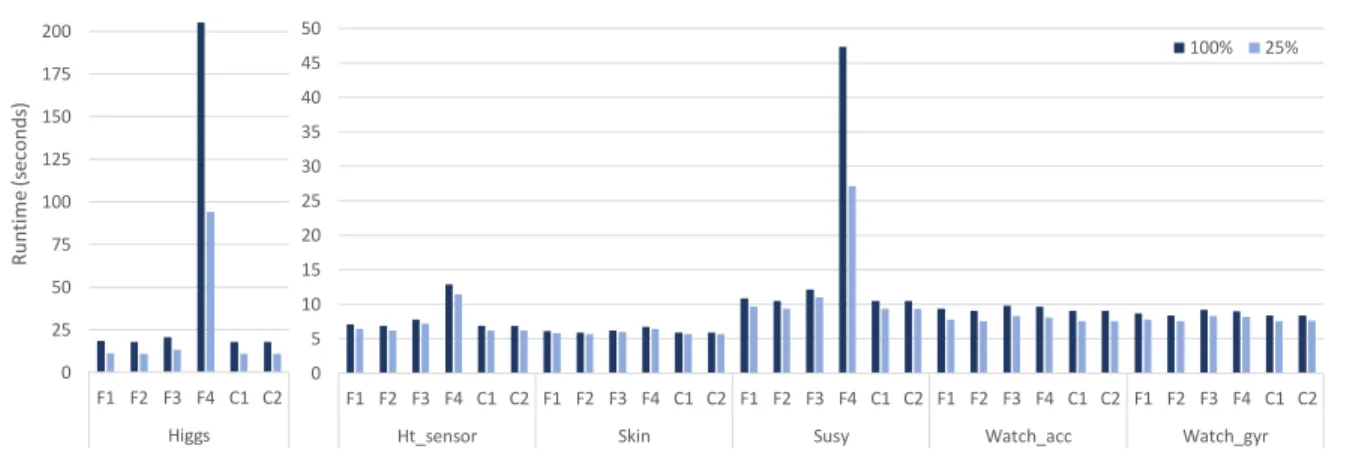
Below we present the runtime results of classifiers and met-rics, with the aim of analyzing the scalability of the models and the influence of the number of samples. Figures 3 and 4 plot the runtime for literature metrics and our proposals, respectively, showing for each of them the 4 sub-sampling levels.

According to these runtimes, we extract the following analysis:

• The metrics in the literature have very fast runtimes, reaching a maximum of approximately 200 seconds for the Higgs dataset. In addition, the difference between the runtime of 100% of the data and 25% is not very high, which shows an excelent scalability of the metrics. • In relation to the proposed metrics, ND obtains higher runtimes than the other metrics. In addition, it increases considerably if we compare 25% against 100%. This shows how the number of instances affects runtime.

(9)

0 5 10 15 20 25 30 35 40 45 50 F1 F2 F3 F4 C1 C2 F1 F2 F3 F4 C1 C2 F1 F2 F3 F4 C1 C2 F1 F2 F3 F4 C1 C2 F1 F2 F3 F4 C1 C2

Ht_sensor Skin Susy Watch_acc Watch_gyr

100% 25% 0 25 50 75 100 125 150 175 200 F1 F2 F3 F4 C1 C2 Higgs R un ti m e (s ec o nd s)

FIGURE 3:Runtime of literature metrics

0 2000 4000 6000 8000 10000 12000 Higgs Susy R unt im e (s ec o nds ) 0 100 200 300 400 500 600 700

Ht_sensor Skin Watch_acc Watch_gyr 100% 75% 50% 25%

(a)ND: Neighborhood Density

0 50 100 150 200 250 300 350 Higgs Susy R unt im e (s ec o nds ) 0 10 20 30 40 50 60 70 80

Ht_sensor Skin Watch_acc Watch_gyr 100% 75% 50% 25%

(b)DTP: Decision Tree Progression

FIGURE 4:Runtime of proposed metrics

0 100 200 300 400 500 600 700 LH S-Fk N N _DT M LP Higgs R un ti m e (s ec o nd s) 0 20 40 60 80 100 120 140 160 180 200 LH S-Fk N N _DT M LP LH S-Fk N N _DT M LP LH S-Fk N N _DT M LP LH S-Fk N N _DT M LP LH S-Fk N N _DT M LP

Ht_sensor Skin Susy Watch_acc Watch_gyr 100% 25%

FIGURE 5:Runtime of classifiers

DTP is faster than ND and is more robust in scalability, as it is less affected by the number of instances. It is very important to remember the results obtained in the previous section, where it is shown that ND and DTP are the metrics that provide best information to the problem. Thus, obtaining the values of the proposed metrics allows us to know if we are facing problems

where we can discard instances and keep the results very close.

After analyzing the scalability of the metrics, it is neces-sary to analyze the impact of the instance reduction in the classifiers. For this purpose, Figure 5 shows the runtime of the three classifiers with the 6 datasets, for their full version (100%) and maximum subsample applied (25%).

As expected, all the algorithms show a great reduction in runtime. LHS-FkNN and MLP achieve the greatest reduction in runtime. The reason is the LHS-FkNN algorithm is an instance-based method and reducing the number of instances decreases the number of comparisons to be made at the classification stage. On the other hand, MLP is based on weighting through an iterative process, for this reason, a high number of instances is affected in complexity by the number of iterations performed to train the model. DT remains more stable, slightly affected by the number of instances due to the design of the algorithm to train the tree in a distributed way.

The most relevant analysis that can be extracted involves the runtime. The time spent in obtaining the metrics can lead us to the conclusion of reducing the dataset by half, or keeping only 25% without significantly affecting the quality of the classifier. In addition, it allows us to perform more

(10)

experiments to determine which is the algorithm that learns most about our problem and optimize the parameters of the classifiers. For example, we can see a realistic scenario: we find a problem where the ND and DTP metrics obtain low values, and in addition the C1 and C2 metrics show us a class imbalance problem. We can apply random undersampling, to produce a balance between classes and improve the quality of the results. Moreover, by reducing the size of the dataset, we can spend more time on finding a better solution to the problem, such as using preprocessing techniques to filter noisy instances or optimize the parameters of the classifier.

VI. CONCLUSIONS AND FURTHER WORK

In this paper, two metrics have been proposed to study the complexity and density in big data problems: ND and DTP study density and accuracy progression by discarding half of the samples randomly. In addition, some basic metrics have been adapted from the literature to handle big dataset. The design based on Spark allows us to characterize large datasets in a short period of time, obtaining valuable information. The developed metrics are available in the open source repos-itory Spark-packages called ComplexityMetrics at: https:// spark-packages.org/package/JMailloH/ComplexityMetrics

According to the study carried out through the proposed metrics, it is common for big datasets to show redundancy information in their samples. This high redundancy allows us to reduce the size to 25% of the samples without drastically affecting the accuracy obtained by the classifiers, achieving a significant faster runtimes. This shows that the number of instances in big datasets used is more than necessary, and highlights the need to prioritize preprocessing techniques to obtain smart data.

As a final conclusion, we have to emphasize the fact of redundancy in many big data classification problems, where with a much smaller set, a small quality dataset, we can have similar or better results. Here the challenge is in obtaining smart data with the minimum necessary size.

As future work we believe that the proposed metrics have a great potential to be integrated in the area of auto machine learning techniques [19] in the big data context. A good starting point would be to design a technique that allows us to determine the necessary size to tackle a big data classifica-tion problem, reducing the number of instances significantly without affecting the results obtained, toward a reduced smart data.

In addition, complexity metrics similar to DTP can be developed by changing the base classifier, to study how the reduction of the dataset affects other classifier families.

ACKNOWLEDGMENTS

This contribution has been supported by the Spanish National Research Project TIN2017-89517-P. J. Maillo hold a FPU scholarship from the Spanish Ministry of Education.

REFERENCES

[1] T. B. Ho, “Knowledge discovery,” inKnowledge Science. CRC Press, 2016, pp. 70–93.

[2] P. V. Coveney, E. R. Dougherty, and R. R. Highfield, “Big data need big theory too,”Philosophical Transactions of the Royal Society A: Mathemat-ical, Physical and Engineering Sciences, vol. 374, no. 2080, p. 20160153, 2016.

[3] R. J. Gonzalez, “Hacking the citizenry?: Personality profiling, big data and the election of donald trump,”Anthropology Today, vol. 33, no. 3, pp. 9– 12, 2017.

[4] Z. Tufekci, “Big questions for social media big data: Representativeness, validity and other methodological pitfalls,” inEighth International AAAI Conference on Weblogs and Social Media, 2014.

[5] T. B. Murdoch and A. S. Detsky, “The inevitable application of big data to health care,”Jama, vol. 309, no. 13, pp. 1351–1352, 2013.

[6] J. A. Ramos, J. B. Rollins, and D. G. Wilhite, “Smart data caching using data mining,” Mar. 22 2011,Google PatentsUS Patent 7,912,812. [7] D. Ardagna, C. Cappiello, W. Samá, and M. Vitali, “Context-aware data

quality assessment for big data,”Future Generation Computer Systems, vol. 89, pp. 548–562, 2018.

[8] S. García, J. Luengo, and F. Herrera, Data preprocessing in data mining. Springer, 2015.

[9] I. Triguero, D. García-Gil, J. Maillo, J. Luengo, S. García, and F. Herrera, “Transforming big data into smart data: An insight on the use of the k-nearest neighbors algorithm to obtain quality data,”Wiley Interdisciplinary Reviews: Data Mining and Knowledge Discovery, vol. 9, no. 2, p. e1289, 2019.

[10] T. M. Cover, P. Hart et al., “Nearest neighbor pattern classification,”IEEE transactions on information theory, vol. 13, no. 1, pp. 21–27, 1967. [11] J. Luengo, S. García, and F. Herrera, “On the choice of the best imputation

methods for missing values considering three groups of classification methods,”Knowledge and Information Systems, vol. 32, no. 1, pp. 77–108, 2012.

[12] M. H. ur Rehman, C. S. Liew, A. Abbas, P. P. Jayaraman, T. Y. Wah, and S. U. Khan, “Big data reduction methods: a survey,”Data Science and Engineering, vol. 1, no. 4, pp. 265–284, 2016.

[13] D. García-Gil, F. Luque-Sánchez, J. Luengo, S. García, and F. Herrera, “From big to smart data: Iterative ensemble filter for noise filtering in big data classification,”International Journal of Intelligent Systems, vol. 34, no. 12, pp. 3260–3274, 2019.

[14] Z. Liu, Q. Pan, J. Dezert, and G. Mercier, “Hybrid classification system for uncertain data,”IEEE Transactions on Systems, Man, and Cybernetics: Systems, vol. 47, no. 10, pp. 2783–2790, Oct 2017.

[15] T. Denœux, S. Sriboonchitta, and O. Kanjanatarakul, “Evidential cluster-ing of large dissimilarity data,”Knowledge-Based Systems, vol. 106, pp. 179 – 195, 2016.

[16] L. P. F. Garcia, A. C. Lorena, M. C. P. de Souto, and T. K. Ho, “Classifier recommendation using data complexity measures,” in24th International Conference on Pattern Recognition (ICPR), Aug 2018, pp. 874–879. [17] I. Muslea, S. Minton, and C. A. Knoblock, “Selective sampling with

redundant views,” inAAAI/IAAI, 2000, pp. 621–626.

[18] M. Sugiyama, T. Suzuki, and T. Kanamori, Density ratio estimation in machine learning. Cambridge University Press, 2012.

[19] F. Hutter, L. Kotthoff, and J. Vanschoren, Automated Machine Learning. Springer, 2019.

[20] M. Feurer, A. Klein, K. Eggensperger, J. T. Springenberg, M. Blum, and F. Hutter, Auto-sklearn: Efficient and Robust Automated Machine Learning. Cham:Springer International Publishing, 2019, pp. 113–134. [21] A. C. Lorena, L. P. Garcia, J. Lehmann, M. C. Souto, and T. K. Ho, “How complex is your classification problem?: A survey on measuring classification complexity,” ACM Computing Surveys (CSUR), vol. 52, no. 5, p. 107, 2019.

[22] L. P. Garcia, A. C. de Carvalho, and A. C. Lorena, “Effect of label noise in the complexity of classification problems,”Neurocomputing, vol. 160, pp. 108–119, 2015.

[23] A. Hoekstra and R. P. Duin, “On the nonlinearity of pattern classifiers,” inProceedings of 13th International Conference on Pattern Recognition, vol. 4. IEEE, 1996, pp. 271–275.

[24] M. Zaharia, M. Chowdhury, T. Das, A. Dave, J. Ma, M. McCauly, M. J. Franklin, S. Shenker, and I. Stoica, “Resilient distributed datasets: A fault-tolerant abstraction for in-memory cluster computing,” inPresented as part of the 9th USENIX Symposium on Networked Systems Design and Implementation NSDI 12, 2012, pp. 15–28.

(11)

[25] A. Orriols-Puig, N. Macia, and T. K. Ho, “Documentation for the data complexity library in c++,” Ph.D. dissertation, Universitat Ramon Llull, La Salle, 2010.

[26] R. A. Mollineda, J. S. Sánchez, and J. M. Sotoca, “Data characterization for effective prototype selection,” inIberian Conference on Pattern Recog-nition and Image Analysis. Springer, 2005, pp. 27–34.

[27] L. Cummins, “Combining and choosing case base maintenance algo-rithms,” PhD Thesis, University College Cork, 2013.

[28] A. C. Lorena, I. G. Costa, N. Spolaôr, and M. C. De Souto, “Analysis of complexity indices for classification problems: Cancer gene expression data,”Neurocomputing, vol. 75, no. 1, pp. 33–42, 2012.

[29] N. V. Chawla, Data Mining for Imbalanced Datasets: An Overview. Boston, MA: Springer US, 2010, pp. 875–886.

[30] A. K. Tanwani and M. Farooq, “Classification potential vs. classification accuracy: a comprehensive study of evolutionary algorithms with biomed-ical datasets,” inLearning Classifier Systems. Springer, 2009, pp. 127– 144.

[31] A. Fernández, S. García, M. Galar, R. C. Prati, B. Krawczyk, and F. Her-rera, Learning from imbalanced data sets. Springer, 2018.

[32] J. Maillo, S. Ramírez, I. Triguero, and F. Herrera, “kNN-IS: an iterative spark-based design of the k-Nearest Neighbors classifier for big data,” Knowledge-Based Systems, vol. 117, pp. 3–15, 2017.

[33] Spark packages contributors, “Spark Packages: A community index of third-party packages for Apache Spark,” 2020, https://spark-packages. org/, [Online; accessed 15 January 2020].

[34] J. Dean and S. Ghemawat, “Map Reduce: A flexible data processing tool,” Communications of the ACM, vol. 53, no. 1, pp. 72–77, 2010.

[35] C.-F. Tsai, W.-C. Lin, and S.-W. Ke, “Big data mining with parallel computing: A comparison of distributed and mapreduce methodologies,” Journal of Systems and Software, vol. 122, pp. 83 – 92, 2016.

[36] X. Meng, J. Bradley, B. Yavuz, E. Sparks, S. Venkataraman, D. Liu, J. Freeman, D. Tsai, M. Amde, S. Owen, and et al., “Mllib: Machine learning in apache spark,”The Journal of Machine Learning Research, vol. 17, no. 1, p. 1235–1241, Jan. 2016.

[37] D. Dua and C. Graff, “UCI machine learning repository,” 2017. [Online]. Available: http://archive.ics.uci.edu/ml

[38] S.-J. Yen and Y.-S. Lee, Under-Sampling Approaches for Improving Prediction of the Minority Class in an Imbalanced Dataset. Springer Berlin Heidelberg, 2006, pp. 731–740.

[39] J. Maillo, S. García, J. Luengo, F. Herrera, and I. Triguero, “Fast and scalable approaches to accelerate the fuzzy k nearest neighbors classifier for big data,”IEEE Transactions on Fuzzy Systems, 2019 - In press.

JESUS MAILLO received the B.Sc. and M.Sc.

degrees in computer science from the University of Granada, Granada, Spain, in 2014 and 2015. He is currently pursuing the Ph.D. degree in the De-partment of Computer Science and Artificial Intel-ligence in the University of Granada. His research interests include data mining, data preprocessing and big data.

ISAAC TRIGUERO received his M.Sc. and

Ph.D. degrees in Computer Science from the Uni-versity of Granada, Granada, Spain, in 2009 and 2014, respectively. He is currently an Assistant Professor of Data Science since June 2016. His work is mostly concerned with the research of novel methodologies for big data analytics. Dr Triguero has published more than 70 international publications in the fields of Big Data, Machine Learning and Optimisation (H-index=24 and more than 2200 citations on Google Scholar). He is a Section Editor-in-Chief of the Machine Learning and Knowledge Extraction journal, and an associate editor of the Big Data and Cognitive Computing journal, and the IEEE Access journal. He has acted as Program Co-Chair of the IEEE Conference on Smart Data (2016), the IEEE Conference on Big Data Science and En-gineering (2017), and the IEEE International Congress on Big Data (2018). Dr Triguero is currently leading a Knowledge Transfer Partnership project funded by Innovative UK and the energy provider E.ON that investigates Smart Metering data.

FRANCISCO HERRERA(SM’15)received his

M.Sc. in Mathematics in 1988 and Ph.D. in Math-ematics in 1991, both from the University of Granada, Spain. He is a Professor in the Depart-ment of Computer Science and Artificial Intelli-gence at the University of Granada and Director of the Andalusian Research Institute in Data Science and Computational Intelligence (DaSCI). He’s an academician in the Royal Academy of Engineer-ing (Spain).

He has been the supervisor of 49 Ph.D. students. He has published more than 500 journal papers, receiving more than 82000 citations (Scholar Google, H-index 139). He has been selected as a Highly Cited Researcher (in the fields of Computer Science and Engineering, respectively, 2014 to present, Clarivate Analytics).

He currently acts as Editor in Chief of the international journal "Informa-tion Fusion" (Elsevier). He acts as editorial member of a dozen of journals.

He received the several honors and awards, among others: ECCAI Fellow 2009, IFSA Fellow 2013, 2010 Spanish National Award on Computer Science ARITMEL to the "Spanish Engineer on Computer Science", In-ternational Cajastur "Mamdani" Prize for Soft Computing (Fourth Edition, 2010), IEEE Transactions on Fuzzy System Outstanding 2008 and 2012 Paper, 2011 Lotfi A. Zadeh Prize Best paper Award (IFSA Association), 2013 AEPIA Award to a scientific career in Artificial Intelligence, 2014 XV Andalucía Research Prize Maimónides, 2017 Andalucía Medal (by the regional government of Andalucía), 2018 “Granada: Science and Innovation City” award.

His current research interests include among others, Computational In-telligence (including fuzzy modeling, computing with words, evolutionary algorithms and deep learning), information fusion and decision making, and data science (including data preprocessing, prediction, singular problems, and big data).