QUANTIFYING RIVER FORM VARIATIONS IN THE MISSISSIPPI BASIN USING REMOTELY SENSED IMAGERY
Zachary F. Miller
A thesis submitted to the faculty at the University of North Carolina at Chapel Hill in partial fulfillment of the requirements for the degree of Master of Science in the Department of
Geological Sciences.
Chapel Hill 2013
Approved by:
Tamlin M. Pavelsky
Jonathan M. Lees
ABSTRACT
Zachary F. Miller: Quantifying River Form Variations in the Mississippi Basin Using Remotely Sensed Imagery
(Under the direction of Tamlin M. Pavelsky)
Geographic variations in river shape are often estimated using the framework of
downstream hydraulic geometry (DHG), which links spatial changes in discharge and channel
width, depth, and velocity through power-law models. Because these empirical relationships are
derived from in situ data and may not describe all variability in channel form, we create a dataset
of 1.2x10⁶ river widths in the Mississippi Basin measured from remotely sensed imagery. We
construct DHG for the Mississippi drainage by linking DEM-estimated discharge values to each
width measurement. Well-developed DHG exists over the entire Mississippi basin, while
individual sub-basins vary substantially from existing width-discharge scaling. Comparison of
depth predictions from traditional depth-discharge relationships with one incorporating width
into the DHG framework shows that including width improves depth estimates in basins with
high width variability. Results suggest that channel geometry derived from remotely sensed
ACKNOWLEDGEMENTS
I would like to thank my advisor, Dr. Tamlin Pavelsky, for his guidance and support
during this thesis project. Dr. Ben Mirus and Dr. Jonathan Lees provided valuable feedback and
comments on the paper. Dr. Jason Barnes was an excellent resource during the research phase of
the project. Funding for this project was provided through NASA New Investigator Grant
#NNX12AQ77G to Dr. Tamlin Pavelsky and by the UNC Department of Geological Sciences
Martin Fund. Finally, I thank my family for their support and encouragement throughout this
TABLE OF CONTENTS
LIST OF FIGURES ... vii
LIST OF TABLES ... viii
LIST OF SYMBOLS AND ABBREVIATIONS ... ix
CHAPTER I: Quantifying River Form in the Mississippi Basin Using Remotely Sensed Imagery ... 1
1. INTRODUCTION ... 1
2. DOWNSTREAM HYDRAULIC GEOMETRY: A BRIEF REVIEW ... 5
3. DATA AND METHODS ... 7
3.1 Calculating River Widths ... 7
3.2 Estimating river discharge ... 9
3.3 Construction of downstream hydraulic geometry ... 10
3.4 Width validation ... 12
3.5 Depth estimation ... 12
4. RESULTS ... 13
4.1 Measurement and distribution of river widths ... 13
4.2 Width measurement accuracy ... 16
4.3 Estimation of discharge ... 18
4.4 Mississippi Basin downstream hydraulic geometry ... 20
4.5 Estimating depth ... 21
LIST OF FIGURES
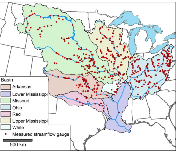
Figure 1. Major sub-basins of the Mississippi and USGS gauging stations ... 4
Figure 2. Inputs, intermediate steps, and products for calculation of river width ... 8
Figure 3. Discharge-drainage area relationships for sub-basins of the Mississippi ... 10
Figure 4. Linking RivWidth and DEM measurements ... 11
Figure 5. Mississippi Basin width map ... 14
Figure 6. Width distributions in the Mississippi Basin ... 14
Figure 7. Percentage of USGS gauging stations measured in this study ... 16
Figure 8. Width measurement error ... 17
Figure 9. NLCD image of the Upper Mississippi River near MacGregor, IA ... 18
Figure 10. Estimated and USGS measured mean discharges for 346 gauging stations in the Mississippi basin. ... 19
Figure 11. Density plots of width versus discharge for the Ohio, Upper Mississippi, Missouri, and entire Mississippi basin ... 21
Figure 12. 8 x 10⁵ mean depths in the Mississippi basin estimated using multiple regression ... 22
LIST OF TABLES
Table 1. Measurement coverage and density ... 15
Table 2. Estimated discharge-measured discharge regressions ... 19
LIST OF SYMBOLS AND ABBREVIATIONS
A ... Drainage area
a ... Width coefficient
b ... Width exponent
c ... Depth coefficient
d ... Channel depth
DEM ... Digital elevation model
DHG ... Downstream hydraulic geometry
f ... Depth exponent
k ... Velocity coefficient
m ... Velocity exponent
n ... Number of measurements
MAE ... Mean absolute error
NLCD ... National Land Cover Dataset
Q ... Channel discharge
v ... Channel velocity
w ... Channel width
CHAPTER 1: QUANTIFYING RIVER FORM IN THE MISSISSIPPI BASIN USING REMOTELY SENSED IMAGERY
1. INTRODUCTION
Rivers systems connect the terrestrial and oceanic reservoirs of the hydrologic cycle and
play a crucial role in landscape development and freshwater resources. Because spatial changes
in river form are physical expressions of interaction between a river’s flow and the surrounding
environment, they are critical to a wide range of scientific and engineering fields. For example,
channel geometry, which includes the key variables of width, depth, velocity, and slope, reflects
local and regional uplift in bedrock and alluvial rivers and responds to changes in bedrock
lithology [Whipple, 2004; Montgomery, 2004; Harbor, 1998; Amos and Burbank, 2007;
Montgomery and Gran, 2001]. River width and depth play a vital role in CO2 and nutrient
exchange [Butman and Raymond, 2011; Alexander et al, 2000; Wollheim, et al., 2006; Peterson
et al., 2001]. Aquatic habitat distribution is largely dependent on channel geometry, which both
influences the spatial extent of habitats and acts as a barrier to terrestrial species migration
[Jowett, 1998; Newson and Newson, 2000; Ayres and Clutton-Brock, 1992; Hayes and Sewlal,
2004]. Humans depend on accurate assessments of river form for understanding flooding
hazards, transportation planning, and fisheries management [Hobley, et al., 2012; Apel, et al.,
2009; McCartney, 1986; Troitsky, 1994; Prevost et al., 2003]. Channel shape is also a principal
parameter in hydrologic and hydrodynamic models [Paiva, et al., 2013; Neal et al., 2012;
spatial patterns of channel shape have been studied for more than a century [Humphreys and
Abbott, 1867; Bellasis, 1913].
The framework of downstream hydraulic geometry (DHG), developed by Leopold and
Maddock [1953], relates spatial patterns of river form to variations in constant-frequency
discharge throughout a basin. Three fundamental power-law equations relate width (w), depth
(d), and velocity (v) to downstream changes in discharge (Q):
! =!!! (1a)
! =!!! (1b)
! =!!! (1c)
where b, f, m,a, c, and k are empirically calculated exponents and coefficients. To facilitate
comparison of channel shapes over a large geographic extent, the discharge used in DHG is
spatially variable and considered to be of a magnitude equaled or exceeded the same percent of
time at different locations. Due to the difficulty in obtaining spatially continuous measurements
of channel geometry, these relationships are often used to estimate channel characteristics in
studies of landscape evolution [Tucker and Bras, 1998], nutrient flux [Butman and Raymond,
2011; Carleton and Mohamoud, 2013], width distributions [Andreadis, et al., 2013] and the
movement of materials, energy, and organisms [Sabo and Hagen, 2012].
Traditional investigations of geographic variability in equilibrium channel form rely on in
situ measurements of river geometry, which are usually available only at widely-spaced
locations. This methodology faces two fundamental obstacles in characterizing spatial variations
in width and depth. First, the time-intensive nature of in situ channel measurement limits the
number of data points to a maximum of hundreds [Moody and Troutman, 2002] to thousands
[e.g. Wolman, 1955] or the density of measurements to wide spacing over larger areas [e.g.
Moody and Troutman, 2002; Leopold and Maddock, 1953]. Second, in situ channel
measurements are often acquired at permanent streamflow gauging sites where accuracy of
discharge measurements is usually prioritized, potentially biasing site selection towards desired
features such as stable, single-channel cross-sections that may not accurately represent the full
range of channel characteristics [Rantz, 1982; Ibbitt, 1997]. These factors suggest that traditional
investigations of river shape may not always encompass the full range of spatial variability in
channel geometry.
Due to the importance of river form and the difficulty of obtaining wide-scale in situ
channel measurements, remote sensing has increasingly been used to characterize river width,
depth, and velocity [e.g. Legleiter, 2012; Fonstad and Marcus, 2005; Pavelsky and Smith, 2009;
Mersel, et al., 2013]. As the river parameter most readily observable from remotely sensed data,
river width has been quantified using a variety of passive and active sensors since the early
stages of the Landsat satellite program in the 1970s [Rango and Salomonson, 1974; Watson,
1991; Smith et al., 1996, Allen et al., 2013]. While remote sensing of channel width has
generally covered single rivers or limited spatial extents, recognition of the potential for
large-scale width measurement has recently led to regional and global studies [Pavelsky, et al., in
review; Yamazaki, et al., in review; Andreadis, et al., 2013].
The RivWidth software tool provides automated and spatially continuous channel width
measurements from a variety of data sources at the native image resolution [Pavelsky and Smith,
2008]. In this study, we use RivWidth and the Landsat-based National Land Cover Dataset
(NLCD) to quantify the spatial variability of river width at a constant-frequency discharge in the
measurements with mean annual discharge values estimated from discharge-drainage area
relationships to construct DHG relationships for the basin as a whole and for major sub-basins.
Finally, we use our measured widths and estimated discharge values and in situ channel width,
area, and discharge measurements from U.S. Geological Survey (USGS) streamflow gauging
stations to estimate continuous mean channel depths using a multiple linear regression
framework. With these high-resolution, spatially extensive datasets we both test the large-scale
applicability of the power laws of downstream hydraulic geometry and create a dataset that
replaces DHG-based estimates in many applications.
2. DOWNSTREAM HYDRAULIC GEOMETRY: A BRIEF REVIEW
The first studies of river form focused on quantifying equilibrium channel shapes in
man-made canals that balanced discharge, width, and sediment load for engineering purposes [Lacey,
1930]. The modern framework of downstream hydraulic geometry was proposed by Leopold
and Maddock [1953] to explain large-scale changes in channel form and applied to a range of
natural rivers. Since then, the initial power-law relationships have been expanded to include
sediment properties, slope, and shear stress [Ferguson, 1986; Lee and Julien, 2006]. In addition
to hydrologic analyses of spatial changes in river from and flow, DHG is now commonly used in
studies linking channel networks with formation of the landscapes they create [Attal et al., 2008;
Tucker and Hancock, 2010; Allen et al., 2013].
Investigations of discharge and channel geometry show consistent relationships between
width and increasing downstream flow. Lacey [1930] found width in stable canals to vary with
the square root of discharge, while numerous subsequent analyses of natural channels obtained
similar width exponents (b ≈ 0.5, Equation 1a), as well as consistency in depth and velocity
exponents (f ≈ 0.4; m ≈ 0.1, Equations 1b,c) [Leopold and Maddock, 1953; Leopold and Miller,
1956; Stall and Fok, 1968; Moody and Troutman, 2002; Chaplin, 2005]. Although these studies
find similarity of DHG exponents across a wide range of river sizes and settings, coefficients a,
c, and k vary for individual basins, regions, or spatial scales [Leopold and Maddock, 1953;
Moody and Troutman, 2002]. While DHG relationships were initially empirical, observed
consistency in exponents led to theoretical explanations based on minimum energy expenditure
in conjunction with sediment transport and slope-area discharge methods like the
Manning-Strickler formula [Yang et al., 1981; Ferguson, 1986; Molnar and Ramirez, 2002; Eaton and
Other studies finding either substantial variation in DHG exponents or high variability in
channel shape unrelated to discharge suggest that the framework sometimes fails to capture
variations in river form. Exponents deviating substantially from previously assumed values are
often related to variations in basin size, tectonic activity, bedrock lithology, channel vegetation,
and levels of human influence [Park, 1977; Klein, 1981; Montgomery and Gran, 2001;
Montgomery, 2004; Piestch and Nanson, 2011]. Wohl [2004] found evidence that
“well-developed” DHG (defined as two of the three primary hydraulic variables having r2 values
greater than 0.5 in relation to discharge) exists where the stream power to sediment size ratio is
high, implying that the erosive potential of a river relative to its bank strength governs its ability
to adjust channel geometry to increasing flow. Finally, the framework of DHG does not provide
for channel narrowing downstream, a characteristic observed in rivers crossing tectonic or
lithologic discontinuities [Harbor, 1998; Montgomery and Gran, 2001; Allen, et al., 2013].
These deviations from DHG highlight its limitations in describing large-scale variations in river
form.
Development of DHG relationships in a basin requires measurements of channel
variables at constant-frequency discharge [Leopold and Maddock, 1953]. While bankfull
discharge is often used in DHG studies because it approximates the dominant channel-forming
flow [e.g. Wolman, 1955; Leopold and Miller, 1956; Chaplin, 2005; Pietsch and Nanson, 2011],
other constant-frequency discharges such as mean annual discharge have also been used
successfully [Leopold and Maddock, 1953; Griffiths, 1980; Molnar and Ramirez, 2002]. While
mean annual flows are usually lower than channel-forming discharges, comparison of DHG
exponents from a range of flow frequencies shows only minor variation [Knighton, 1974;
3. DATA AND METHODS 3.1. Calculating river widths
The RivWidth software tool, described in detail by Pavelsky and Smith [2008], is an
algorithm implemented in the IDL programming language that calculates a continuous sequence
of river centerline pixels and channel width perpendicular to flow at each pixel. To extract river
width data, the RivWidth software tool requires a binary image of inundation extent. Both the
minimum river size measured and accuracy of RivWidth are highly dependent on the resolution
of the imagery used. Previous studies have used inputs from MODIS, Landsat, and SPOT-5
satellite images [Pavelsky and Smith, 2008; Smith and Pavelsky, 2008; Allen et al., 2013]. In this
study, we use the open water classification from the U.S. Geological Survey’s National Land
Cover Dataset (NLCD). The NLCD is a continuous land cover classification based on tasseled
cap transformations of Landsat 5 and 7 satellite imagery for three growing seasons [Homer et al.,
2004]. While ideal data for this study would include images from known periods of mean annual
or bankfull discharge, we hypothesize that the NLCD water classification depicts rivers in an
approximately mean discharge state because it represents an integration of river extent from
early, peak, and late growing seasons. We test this hypothesis as described in sections 3.4 and
4.2. Although the extreme northernmost portion of the Mississippi Basin extends slightly
outside the coverage of the NLCD into Canada, this area is not included in our analysis because
the techniques used to classify open water would be inconsistent with the rest of the basin.
To prepare the NLCD water class for input into RivWidth, the open water classification
was masked using the ENVI software suite (Figure 2a, 2b) and subset into major hydrologic
regions as defined in the USGS’s hydrologic unit code system [Seaber et al., 1987]. These
(Missouri/Arkansas-Red—14N; Upper and Lower Mississippi—15N; Ohio—17N) and further divided into
hydrologic accounting units (~3 x 10⁴ km2). To create as complete and continuous a dataset as
possible, bridges and other small gaps were manually filled.
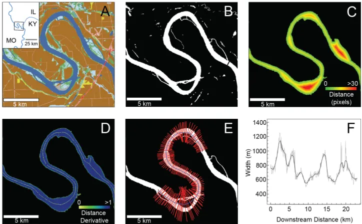
Figure 2: Inputs, intermediate steps, and products for calculation of river width in this study: A) National Land Cover Dataset; B) binary water mask of the open water classification; C) distance image based on a filled channel mask; D) derivative of distance image used to calculate the centerline; E) flow width measurements along orthogonal line segments to each centerline pixel; F) plot of raw (grey) and smoothed (black) continuous widths.
For each accounting unit, RivWidth then automatically executes five steps. It 1) creates a
channel mask by removing water bodies not connected to the river channel; 2) fills in islands in
the channel to create a mask of spatial river extent; 3) determines the distance from each river
pixel to the nearest non-river pixel and calculates the derivative of the resulting distance image
(Figure 2c, 2d); 4) determines the river centerline based on the derivative map, in which
centerline pixels have values close to zero and all other river pixels have values of approximately
each centerline pixel (Figure 2e). For this study, start points and endpoints of 320 individual
river segments were manually selected to exclude in-channel lakes and reservoirs. The final
RivWidth output is a text file containing widths, the associated UTM coordinates, and the
number of river channels in the cross-section. Further descriptions, updates and downloads are
available from Pavelsky and Smith [2008] and at http://www.unc.edu/~pavelsky/.
3.2. Estimating river discharge
In addition to channel width, construction of DHG relationships requires knowledge of
downstream changes in constant-frequency discharge. Because spatially continuous river
discharge is not currently measurable, we use drainage area (A) as a proxy for flow. A linear
relationship between discharge and contributing area is commonly assumed in studies of stream
power, incision, and downstream hydraulic geometry in smaller basins [Pazzaglia et al., 1998;
Montgomery and Gran, 2001]. Drainage area was calculated for 318 channel segments by
extracting river centerlines using USGS HydroSHEDS 3 arc-second (~90 m) digital elevation
models and the hydrology tools in ArcGIS. Once DEM channels were delineated, we sampled
flow accumulation rasters to determine drainage area at each pixel and re-projected the resulting
pixel locations into the appropriate UTM zone for the respective basin. At small spatial scales the
assumption of discharge-drainage area linearity often holds true, but for larger rivers this
relationship may become nonlinear if the basin includes variations in topography, climate, or
land use [Stall and Fok, 1968; Galster et al., 2006; Tague and Grant, 2004]. We develop
discharge-drainage area relationships using values of Q and A for all USGS stations of any
drainage area with ≥10 years of approved mean annual discharge. Because discharge-drainage
calculated least-squares linear regressions for each hydrologic accounting unit in the Ohio,
Upper Mississippi, and much of the Missouri and Lower Mississippi basins. In 7 of the 34
accounting units in the Missouri, 12 of 22 in the Lower Mississippi, and all of the Arkansas basin
(excluding the White River), lack of gauging stations, substantial precipitation variability, or
large-scale water withdrawals precluded gauge-based discharge estimation.
Figure 3: Discharge-drainage area relationships for sub-basins of the Mississippi; exponents close to one indicate a nearly linear fit in the Ohio, Upper and Lower Mississippi sub-basins, but there is substantial deviation from unity in the Missouri and Arkansas sub-basins.
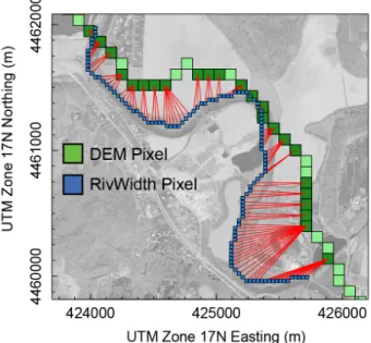
3.3. Construction of downstream hydraulic geometry
Since RivWidth centerlines are based on higher resolution data than Hydrosheds
area relationships therefore required linking each RivWidth measurement to the nearest DEM
pixel. Using the methodology developed by Allen et al. [2013], we assigned the nearest drainage
area value to each RivWidth pixel (Figure 4). Although the two datasets match closely in
comparatively steep channels in the mountainous areas towards the eastern and western
boundaries of the basin, discrepancies of more than a kilometer are common in flatter terrain and
for wider rivers. Once the two datasets were merged, we estimated discharge corresponding to
width measurements using the discharge-drainage area relationships described in section 3.2.
To assess the applicability of Equation 1a in describing width-discharge relationships, we
perform a least-squares linear regression of log-transformed width and discharge. Because the
Mississippi basin contains broad ranges of topography, climate, and human influence, we
investigate these relationships for all available RivWidth measurements and discharge estimates
throughout the basin and individually for the Ohio, Upper Mississippi, and Missouri drainages.
3.4. Width validation
To assess the accuracy of RivWidth measurements and the appropriateness of the NLCD
for describing channel form at mean flows, we compared in situ USGS channel data
corresponding to long-term mean annual discharges to validate width measurements. For many
stations throughout the Mississippi Basin, the USGS measured width, depth, and velocities taken
to develop discharge rating curves are available online [waterdata.usgs.gov/NWIS; Juracek and
Fitzpatrick, 2009]. Although unpublished, these data have been used in investigations of channel
geometry [Bowen and Juracek, 2011; Stover and Montgomery, 2001]. The number of
measurements at each gauge location varies from fewer than ten to thousands across a range of
flows. For each gauge, we estimated the width, depth, and velocity corresponding to mean
annual discharge by calculating the mean value of all channel measurements acquired within
+/-10% of long-term mean annual discharge. Measurements that are clearly erroneous, listed as
“poor” by the USGS, taken more than 60 m (two pixels upstream or downstream from the gauge
location), or measured using a crane along a bridge not perpendicular to the river (therefore not
representing true channel width) were removed. We then projected these gauge locations into
UTM coordinates and calculated total error in our width measurements by comparing in situ
gauge width from the 456 stations meeting our criteria against the mean of the five closest
RivWidth measurements.
3.5. Depth estimation
We evaluated three methods of calculating spatial depth distributions, each using channel
measurements from 358 USGS gauging stations in regions of the Missouri, Upper Mississippi,
available. First, we performed a multiple linear regression of log-transformed in situ depth
against log-transformed in situ width and discharge measurements. We then used our measured
widths and estimated discharge values to calculate depth at each pixel. In previous studies [e.g.
Alexander et al, 2000] depth variations in large river basins have instead been estimated using
traditional DHG relationships, and we develop such a relationship for the Mississippi to evaluate
whether including river width as a variable improves depth estimates over previously used
depth-discharge methods. We also estimate depth using the global depth-depth-discharge equation developed
by Moody and Troutman [2002]. Finally, we assess the effectiveness of including the influence
of width in depth estimation by calculating the mean percentage error of all three depth estimates
relative to USGS-measured depth values at the widest 151 gauging locations. Due to increasing
uncertainty in RivWidth measurements and discharge estimations for smaller rivers, we limited
this depth validation to rivers wider than 100 m.
4. Results
4.1. Measurement and distribution of river widths
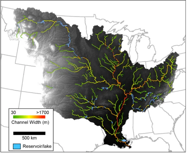
Using the National Land Cover Dataset, we measured 1.194 x 10⁶ individual channel
widths representing 4.2 x 10⁴ km of rivers in the Mississippi basin (Figure 5). Widths ranged
from the minimum pixel size of 30 m to 7400 m in the inundated areas of the Upper Mississippi.
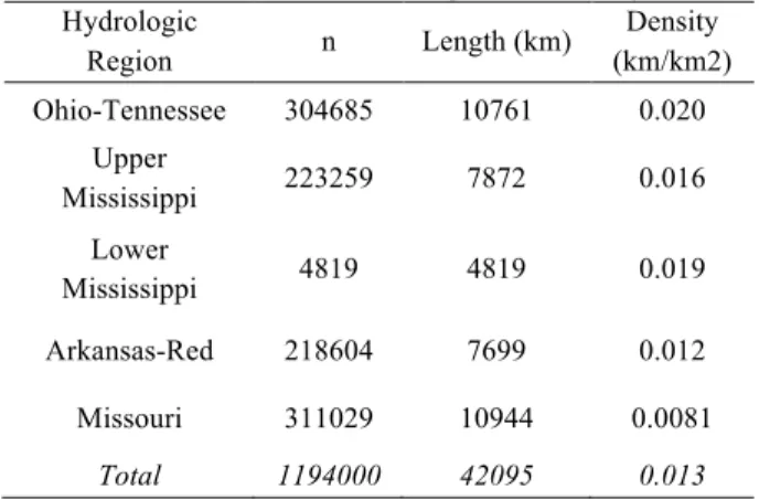
This corresponds to an overall measured drainage density of ~0.013 km/km2. Measurement
count, length and density for each of the five sub-regions of the Mississippi are shown in Table
1. Overall distribution of river widths greater than 100 m and less than 1500 m (Figure 6)
closely follows a negative power-law distribution:
Figure 5: Mississippi River width map (shown with USGS HydroSHEDS DEM) of ~1.2 x 10⁶ observations at 30 m resolution based on the NLCD open water classification.
Table 1: Measurement coverage and density
Hydrologic
Region n Length (km)
Density (km/km2)
Ohio-Tennessee 304685 10761 0.020
Upper
Mississippi 223259 7872 0.016
Lower
Mississippi 4819 4819 0.019
Arkansas-Red 218604 7699 0.012
Missouri 311029 10944 0.0081
Total 1194000 42095 0.013
To evaluate the completeness of this dataset and assess its accuracy, we downloaded
historical channel measurements from 2,466 USGS streamflow gauges taken at long-term mean
annual discharge. Of these, widths are greater than 30 m (the minimum width theoretically
measurable) at 854 locations. Figure 7 shows the percentage of gauges measured in 10 m
increments. Almost all (> 99%) gauge locations wider than 90 m are measured, while the most
substantial decrease occurs as width falls below 60 m (two NLCD pixels). The failure to
measure two 100 m gauges resulted from classification differences in the NLCD (e.g. woody
wetlands rather than open water). At widths between 60 and 100 m, unmeasured stations are
more common because not all channels in this size range are adequately visible in the NLCD for
RivWidth to calculate an accurate river centerline. The rapid reduction in the percentage of
gauges measured at less than 60 m is likely related to difficulties in classifying mixed land-water
pixels, which will often represent the entire river as width decreases below twice the pixel
resolution.
Because USGS gauge station data indicate that RivWidth measured ~68% of gauges
50-100 m, the actual number of channels this size in the basin is likely higher than the number we
(Figure 6). This suggests that although equation (2) is based on width measurements greater
than 100 m, it may also describe the frequency distribution of widths narrower than 100 m.
Figure 7: Percentage of USGS gauging stations measured in this study, binned by in situ channel width; grey fractions indicate number measured out of total gauges per 10-m width range.
4.2. Width measurement accuracy
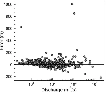
Compared to widths at mean annual discharge from 456 gauging stations in the
Ohio/Tennessee, Upper Mississippi, Missouri, and Arkansas regions, mean absolute width error
(MAE) is 38 m (Figure 8). Because of high variability in USGS measurements and difficulty in
distinguishing channels from inundated floodplains in the Lower Mississippi, gauging stations
not on the main stem are excluded. Total mean and median errors of 20 m and 11 m indicate a
slight positive bias in RivWidth measurements, although outliers with positive errors of more
than 600 m skew these numbers substantially. This error can be partitioned into three groups:
water mask misclassification, RivWidth error, and inaccuracies in USGS measurements. At
gauging stations on the Mississippi River at Winona, MN and MacGregor, IA (Figure 9),
classifies much of the adjacent floodplain as open water. At station 07157950 (Cimarron River
near Buffalo, OK; Q = 3.2 m3/s) USGS measurements of channel width at mean discharge of 26
m contrast with a RivWidth measurement of 651 m. Without these gauges, MAE is reduced to
33 m. While stations with Q > 20 m3/s (n=379) show a relatively small positive bias of only 15
m, stations where Q < 20 m3/s (n=77) have a positive bias of 41 m. This pattern is expected
given that such small rivers approach the narrowest width discernable in 30 m input imagery.
Classification of mixed pixels along banks also imparts a theoretical uncertainty of ½ the pixel
resolution for each bank crossing (i.e. a minimum of 30 m for single-channel rivers at 30 m
resolution; Pavelsky and Smith, 2008).
Figure 8: Width measurement error based on in situ channel measurements from 456 USGS streamflow gauging stations.
Inaccuracies associated with the measurement mechanics of RivWidth are limited to
orthogonal angle errors. Uncertainty results from the predefined spacing of endpoints used to
define orthogonals to each centerline pixel. In highly sinuous channels where centerlines change
direction rapidly, over-measurement can occur when orthogonals are not truly perpendicular to
101 102 103 104
-200 0 200 400 600 800 1000
Discharge (m3/s)
showed that inaccuracies are minimized when 11-pixel centerline segments are used, as we do
here. Finally, although not quantifiable, error associated with US Geological Survey
measurements is minimized through standardized data collection methods [Buchanan and
Somers, 1969; Rantz, 1982] and the careful selection of stations as described in section 3.4.
Figure 9: NLCD image of the Upper Mississippi River near MacGregor, IA; inundated floodplains are extensively connected to channels, leading to high width error.
4.3. Estimation of discharge
Using the methods described in section 3.2, we estimated discharge for rivers totaling 2.8
x 104 km in length and covering 2.2 x 10⁶ km2 of the Mississippi Basin. To assess discharge
accuracy, we compared mean discharges from 346 gauging stations in the measured drainage
area to the mean of the nearest 5 discharge estimations. Figure 10 shows the nearly 1:1
relationships between estimated discharge and gauge-measured discharge for individual
sub-basins and for the entire Mississippi. Because ordinary least-squares linear regressions are
to derive robust linear regressions for each sub-basin (Table 2). We use the non-parametric
Spearman’s ρ to characterize goodness-of-fit, as discharges are not normally distributed.
Regression slopes close to one and strong correlation between predicted and measured values
indicate that estimates of discharge are likely accurate.
Figure 10: Estimated and USGS measured mean discharges for 346 gauging stations in the Mississippi basin.
Table 2: Estimated discharge-measured discharge regressions
Ohio Upper Mississippi/
Lower main stem Missouri Total
Regression y=1.00x-0.59 y=0.98x+1.8 y=0.95x+2.0 y=0.98x+0.8
4.4. Mississippi Basin downstream hydraulic geometry
Using spatially continuous discharge estimates, we construct width-discharge
relationships for the Mississippi Basin and, separately, three of its major sub-basins (Figure
11a-d). Linear least-squares regression of log-transformed width and discharge for the 857,808 width
measurements in the basin shows that their relationship can be described by the power-law
equation:
! =16.0!!.!" (r2 = 0.62) (3)
However, these values include 38654 discharge measurements less than 10 m3/s, which
represents a low discharge for a river greater than 30m wide. 89% (34573) of these
low-discharge measurements are found in the Missouri sub-basin, where braided streams with high
width-depth ratios are common. Of 38 USGS gauging station with mean discharge <10 m3/s,
width is overestimated in all with an mean bias of 52 m (Figure 8). It is then likely that
basin-wide widths for discharges below 10 m3/s are erroneously high. If we remove these anomalous
measurements, the width DHG equation is:
! =13.4!!.!" (r2 = 0.64) (4)
These values of coefficient a and exponent b fall close to the range of values calculated for world
rivers by Moody and Troutman (2002). However, individual sub-basins show substantial
variation from these values, with exponents ranging from 0.3 in the Missouri to 0.63 for the
Upper Mississippi (Figure 11). With the exception of the Missouri, variations in discharge
account for > 50% of width variability (r2 = 0.67 and 0.73 for the Upper Mississippi and Ohio),
indicating that in those sub-basins changes in discharge are the primary control on downstream
Figure 11: Density plots of width versus discharge for the Ohio, Upper Mississippi, Missouri, and entire Mississippi basin. Linear fits represent downstream hydraulic geometry relationships analogous to Equation 1a.
4.5. Estimating depth
Using channel measurements from all gauges located on streams measured by RivWidth
with corresponding discharge estimates, we compared methods of estimating depth with and
without width data. The first method is a simple least-squares linear regression of
log-transformed depth and discharge from the gauge station dataset, which results in a power-law
! = 0.18!!.!" (5)
The second method is a multiple linear regression of transformed depth against
log-transformed discharge and width, which yielded the equation
ln ! =0.44−0.82ln ! +0.83 ln (!) (6)
Figure 12 shows depths calculated from equation 6 for the Ohio, Upper Mississippi, Missouri,
and main stem of the Lower Mississippi using our estimated discharge and measured widths.
Figure 12: 8 x 10⁵ mean depths in the Mississippi basin estimated using multiple regression of d against Q and w; lakes shown in blue.
Basin-wide mean depth error is 40% for the two DHG estimations, and 31% for the
multiple regression method (Table 3). Figures 13a-b compare the percentage error of equation
Moody and Troutman [2002]). Although mean relative error is nearly identical in the Ohio and
Upper Mississippi sub-basins, the two discharge-based methods both substantially overestimate
depth for seven gauging stations along the Platte River in the Missouri sub-basin, leading to
relative errors of 50%. The disparity between approaches in the Missouri accounts for the higher
error of the discharge-based equations in the basin as a whole.
Table 3: Mean absolute depth errors (%)
Sub-basin Equation 5 Equation 6 Troutman
Moody-Ohio 29% 29% 31%
Upper
Mississippi 38% 36% 36%
Missouri 58% 30% 58%
Total 41% 31% 41%
Figure 13: Relative depth error for multiple regression method (circles) and A) DHG estimate (this study); B) DHG estimate (Moody and Troutman, 2002).
5. Discussion and Conclusions
In this study, we present one of the first high-resolution, spatially continuous width
discharge relationships and applications for hydrologic modeling [Pavelsky, et al., in review;
Yamazaki, et al., in review]. Construction of a width frequency distribution using 1.2 x 10⁶
measurements (Equation 2) shows that Mississippi widths follow a power-law distribution
comparable to that found by Pavelsky et al. [in review] for the 8.5 x 10⁵ km2 Yukon basin
(n=1.778x10⁹ W(-1.831) ). Similarities between these two basins—which represent highly
contrasting geology, ecology, climate, and flow regimes—suggest that width distributions in
other basins may follow similar patterns.
Basin-wide width-discharge relationships are characteristic of the downstream hydraulic
geometry framework proposed by Leopold and Maddock [1953]. However, in the global
analysis of Moody and Troutman [2002], changes in discharge account for >94% of width
variation compared to 62% for the Mississippi basin in this study. While error inherent in the
RivWidth dataset undoubtedly accounts for some of the higher width variability observed here, it
seems unlikely that channel width corresponds as precisely to discharge as is shown in previous
work. One explanation for this discrepancy is the widely-spaced and non-random site selection
for in situ channel measurements. To facilitate accurate discharge measurements, USGS gauging
station selection criteria suggest using straight channel segments located away from tributary
junctions, with only one channel and easy access (Rantz, 1982). It is not unreasonable to assume
that similar site selection bias exists for most in situ channel and discharge measurement
locations. In particular, the measurement bias towards single-channel rivers in previous DHG
studies using gauge data may explain the higher width variability observed in this dataset.
Finally, previous investigations of DHG have used datasets incorporating a much wider range of
discharges [e.g. Moody and Troutman, 2002] than the rivers used in this study, which may result
Individual sub-basins demonstrate different levels of adherence to traditional downstream
hydraulic geometry. Missouri sub-basin channel widths increase with discharge at a much lower
rate (b=0.3) than has been found in previous studies (e.g. Leopold and Maddock, 1953; Moody
and Troutman, 2002) with a much lower proportion of width variation explained by discharge
increases (r2=0.44). Conversely, the Ohio sub-basin closely matches previous findings (b=0.48;
r2=0.72). Several factors could explain this discrepancy. Multi-channel rivers are much more
common in the Missouri sub-basin than in the Ohio; despite similar total measured lengths
(Table 1) the Missouri contains nearly 2.5 times as many multi-channel measurements as the
Ohio. While multiple channel crossings increase inherent RivWidth measurement error as
explained in section 4.2, braided streams are also likely to show increased width variability in
response to changes in climate and flow regime [Schumm, 2005]. The Missouri sub-basin also
has some of the highest levels of human influence and control in North America, factors that can
affect variability in channel form. In particular, dam construction has varied but pronounced
effects on channel morphology [Gregory, 2006; Williams and Wolman, 2004]. Williams [1978]
documented highly variable channel narrowing of the Platte River as it crosses the Great Plains
due to upstream flow regulation. We believe human factors across the central section of the
Missouri drainage lead to the high width variability and lower than expected increase in width
with discharge observed in Missouri sub-basin.
Human influence also likely plays a role in the high b-value (0.64) observed in the Upper
Mississippi sub-basin. In larger rivers—particularly along the main stem of the Mississippi—
lock and dam control structures artificially widen the channel or connect it to secondary channels
in its floodplain. Because of difficulties in differentiating the main stem of the Mississippi from
these features are included in the width-discharge dataset (Figure 9). While the high b-value
may not represent the natural width changes, we believe it accurately describes present-day
inundation extent along the Upper Mississippi more effectively than would a lower width
exponent.
In sub-basins with well-developed width-discharge relationships, traditional
depth-discharge DHG predicts depth well without inclusion of additional information on river width.
In the Ohio and Upper Mississippi sub-basins, depth estimates based on the two d-Q
relationships show similar accuracy to that of the multiple regression estimation that incorporates
width (Equation 6). In the Missouri sub-basin, however, both traditional DHG methods
substantially underestimate depth for wide, shallow rivers compared to the multiple regression
analysis. Although basin-wide absolute error is not significantly reduced, consistent
overestimation of depth for these rivers suggest that in applications where depths are based on
downstream hydraulic geometry [e.g. Alexander, 2000], factoring width into depth estimations
substantially reduces uncertainty in drainages like the Missouri that exhibit high width
variability.
Potential errors from multiple sources must be addressed when studying channel form
using remote sensing data. The largest sources of uncertainty in our Mississippi dataset are
inherent to the input imagery. Because higher pixel resolution decreases classification error,
increases total channel length, and decreases the size of smallest rivers measured, selecting
appropriate input data is critical. Figure 7 indicates that all rivers greater than three times the
pixel resolution and substantial numbers of smaller rivers are measured. While our results
suggest that the NLCD represents an approximation of river extent close to mean discharge,
surrounding floodplain, misclassification of channel boundary pixels, or potential use of images
taken during times of higher than mean flows. To reduce the error associated with the input
water mask, future investigations should use a consistent and effective classification scheme on
images taken during periods of the desired flow state. Finally, RivWidth must be configured
properly, as the segment length used to calculate the orthogonal direction can create
non-perpendicular cross-sections when poorly chosen (section 4.2).
Provided these sources of error are addressed, RivWidth offers the capability to measure
river width at a high resolution over large basins with small and predictable error. Despite the
importance of river form and flow, in situ river monitoring capabilities have declined over the
last several decades [Vorosmarty et al., 2001], highlighting the importance of remote sensing
techniques that can produce high-resolution, spatially continuous observations of river channels
over large areas [Alsdorf et al., 2007]. Although significant challenges remain in combining
remotely sensed channel observations into direct measurements of discharge, non-real time
estimations of river flow relying on width measurement have been made [LeFavour and Alsdorf,
2004; Smith and Pavelsky, 2008]. As the most easily observable of the three primary dimensions
of river discharge, understanding variations in width is a critical first step in characterizing
discharge from remotely sensed data.
In addition to its importance in the direct measurement of discharge, remote sensing of
river width contributes to the accuracy of hydrologic and hydraulic modeling. While width
parameters are often characterized through empirically derived discharge relationships [e.g.
Yamazaki, et al., 2011, Andreadis et al., 2013], the utility of widths from satellite imagery in
improving hydraulic modeling of river and floodplain dynamics is increasingly recognized [Neal
and global scales and the importance of rivers in natural and human systems, this paper and its
companion study [Yamazaki, et al., in review] both contribute to the National Aeronautics and
Space Administration’s goal of measuring the spatial and temporal variability in Earth’s surface
water resources [Fu, et al., 2012]. While Yamazaki et al. [in review] focuses on producing
global-scale width measurements applicable to large-scale hydrodynamic modeling, this study
creates a high-resolution channel geometry dataset including rivers as narrow as 30 m. These
two products, combined with ongoing work to produce Landsat-derived width datasets globally,
will allow for more accurate characterization of spatial variability in channel form than is
REFERENCES
Alexander, R. B., R. A. Smith, and G. E. Schwarz (2000), Effect of stream channel size on the delivery of nitrogen to the Gulf of Mexico, Nature, 403(6771), 758-761.
Allen, G.H., J. B. Barnes, T. M. Pavelsky, and E. Kirby (2013), Lithologic and tectonic controls on bedrock channel form at the northwest Himalayan front, J. Geophys. Res. Earth Surf.,
118, doi:10.1002/jgrf20113.
Alsdorf, D. E., E. Rodríguez, and D. P. Lettenmaier (2007). Measuring surface water from space. Rev. Geophys., 45, RG2002, doi:10.1029/2006RG000197.
Amos, C. B., and D. W. Burbank (2007), Channel width response to differential uplift, J. Geophys. Res., 112, F02010, doi:10.1029/2006JF000672.
Andreadis, K. M., G. J-P. Schumann, and T. M. Pavelsky (2013), A simple global river bankfull width and depth database, Water Resour. Res., Accepted Article, doi:
10.1002/wrcr.20440.
Apel, H., G. T. Aronica, H. Kreibich, and A. H. Thieken (2009), Flood risk analyses—how detailed do we need to be?, Natural Hazards, 49(1), 79-98, doi: 10.1007/s11069-008-9277-8.
Attal, M., G. E. Tucker, A. C. Whittaker, P. A. Cowie, and G. P. Roberts (2008), Modeling fluvial incision and transient landscape evolution: Influence of dynamic channel adjustment, J. Geophys. Res., 113, F03013, doi:10.1029/2007JF000893.
Ayres, J. M., and T. H. Clutton-Brock (1992), River boundaries and species range size in Amazonian primates. The American Naturalist, 140(3), 531-537.
Bellasis, E. S. (1913), River and canal engineering: the characteristics of open flowing streams, and the principles and methods to be followed in dealing with them, E. & F. N. Spon, Limited, London.
Bowen, M. W., and K. E. Juracek (2011), Assessment of the Geomorphic Effects of Large Floods Using Streamgage Data: the 1951 Floods in Eastern Kansas, USA, Physical Geography, 32(1), 52-77.
Buchanan, T. J., and W. P. Somers (1969), Discharge measurements at gaging stations, U.S. Geol. Surv. Tech. Water Resour. Invest, Book 3, Chap. A8.
Butman, D., and P.A. Raymond (2011), Significant efflux of carbon dioxide from streams and rivers in the United States. Nature Geoscience, 4(12), 839-842, doi:10.1038/NGEO1294.
Chaplin, J. J. (2005), Development of regional curves relating to bankfull-channel geometry and discharge to drainage area for streams in Pennsylvania and selected areas of Maryland,
U.S. Geol. Surv. Scientific Investigations Report2005-5147, 40pp.
Eaton, B. C., and M. Church (2007), Predicting downstream hydraulic geometry: A test of rational regime theory, Journal of Geophysical Research 112, doi:10.1029/JF000574.
Ferguson, R.I. (1986), Hydraulics and hydraulic geometry, Progress in Physical Geography, 10
(1), 1-31.
Fonstad, M. A., and W. A. Marcus (2005), Remote sensing of stream depths with hydraulically assisted bathymetry (HAB) models, Geomorphology, 72(1), 320-339,
doi:10.1016/j.geomorph.2005.06.005.
Fu, L. L., D. Alsdorf, R. Morrow, E. Rodriguez, and N. Mognard (Eds.) (2012), SWOT: The Surface Water and Ocean Topography Mission: Wide-Swath Altimetric Measurement of Water Elevation on Earth, JPL-Publication 12–05, 228 pp. Jet Propul. Lab., Pasadena, Calif.
Galster, J. C., F. J. Pazzaglia, B. R. Hargreaves, D. P. Morris, S. C. Peters, and R.N. Weisman, (2006), Effects of urbanization on watershed hydrology: The scaling of discharge with drainage area, Geology, 34(9), 713-716, doi: 10.1130/G22633.
Gregory, K. J. (2006), The human role in changing river channels, Geomorphology, 79(3), 172-191, doi:10.1016/j.geomorph.2006.06.018.
Griffiths, G. A. (1980), Hydraulic geometry relationships of some New Zealand gravel bed rivers. Journal of Hydrology (NZ), 19, 106-118.
Harbor, D. J. (1998), Dynamic equilibrium between an active uplift and the Sevier River, Utah, The Journal of Geology, 106(2), 181-194.
Hayes, F. E., and J.A.N. Sewlal (2004), The Amazon River as a dispersal barrier to passerine birds: effects of river width, habitat and taxonomy, J Biogeography, 31(11), 1809-1818.
Hobley, D. E., H. D. Sinclair, and S. M. Mudd (2012), Reconstruction of a major storm event from its geomorphic signature: The Ladakh floods, 6 August 2010, Geology, 40(6), 483-486, doi: 10.1130/G32935.1
Homer, C., C. Huang, L. Yang, B. Wylie, and M. Coan (2004), Development of a 2001 national land cover database for the United States, Photogramm. Eng. Remote Sens, 70, 829-840.
Humphreys, C. A., and L. H. ABBOT, (1867), Report upon the physics and hydraulics of the Mississippi River, US Government Printing Office, Washington, DC.
Ibbitt, R. P. (1997), Evaluation of optimal channel network and river basin heterogeneity
Jowett, I. G. (1998), Hydraulic geometry of New Zealand rivers and its use as a preliminary method of habitat assessment, Regulated Rivers: Research & Management, 14(5), 451-466.
Juracek, K. E., and F. A. Fitzpatrick (2009), Geomorphic applications of stream‐gage information, River Research and Applications, 25(3), 329-347.
Klein, M. (1981), Drainage area and the variation of channel geometry downstream, Earth Surf. Process. Landforms, 6(6), 589-593.
Knighton, A. D. (1974), Variation in width-discharge relation and some implications for hydraulic geometry, Geological Society of America Bulletin,85(7), 1069-1076.
Lacey, G. (1930), Stable channels in alluvium, Proc. Inst. Civil Eng., 229, 259-292.
Lee, J. S., and P. Y. Julien (2006), Downstream hydraulic geometry of alluvial channels, J. Hyd. Eng, 132(12), 1347-1352.
Legleiter, C. J. (2012), Mapping river depth from publicly available aerial images, River Research and Applications, doi:10.1002/rra.2560.
LeFavour, G., and D. Alsdorf (2005), Water slope and discharge in the Amazon River estimated using the shuttle radar topography mission digital elevation model, Geophys. Res. Lett., 32, L17404, doi:10.1029/2005GL023836.
Leopold, L. B. and T. Maddock (1953), The hydraulic geometry of stream channels and some physiographic implications, U.S. Geol. Surv. Prof. Paper, 252.
Leopold, L.B. and J. P. Miller (1956), Ephemeral streams—hydraulic factors and their relation to the drainage net, U.S. Geol. Surv. Prof. Paper 282-a.
McCartney, B. (1986), ”Inland Waterway Navigation Project Design.” J. Waterway, Port, Coastal, Ocean Eng., 112(6), 645–657.
Mersel, M. K., L. C. Smith, K. M. Andreadis, and M. T. Durand (2013), Estimation of river depth from remotely sensed hydraulic relationships, Water Resour. Res., 49, 3165–3179, doi:10.1002/wrcr.20176.
Molnar, P., and J. A. Ramirez (2002), On downstream hydraulic geometry and optimal energy expenditure: case study of the Ashley and Taieri Rivers. J. Hydrology, 259(1), 105-115.
Montgomery, D. R. and K. B. Gran (2001), Downstream variations in the width of bedrock channels, Water Resour. Res., 37, 1841-1846, doi:10.1029/2000WR900393.
Moody, J. A., and B. M. Troutman (2002), Characterization of the spatial variability of channel morphology, Earth Surf. Proc. Land.,27(12), 1251-1266, doi:10.1002/esp.403.
Neal, J., G. Schumann, and P. Bates (2012), A subgrid channel model for simulating river hydraulics and floodplain inundation over large and data sparse areas, Water Resour. Res., 48, W11506, doi:10.1029/2012WR012514.
Newson, M. D., and C. L. Newson (2000), Geomorphology, ecology and river channel habitat: mesoscale approaches to basin-scale challenges, Progress in Physical Geography, 24(2), 195-217.
Paiva, R. C. D., D. C. Buarque, W. Collischonn, M.-P. Bonnet, F. Frappart, S. Calmant, and C. A. B. Mendes (2013), Large- scale hydrologic and hydrodynamic modeling of the Amazon River basin, Water Resour. Res., 49, 1226–1243, doi:10.1002/wrcr.20067.
Park, C. C. (1977), World-wide variations in hydraulic geometry exponents of stream channels: an analysis and some observations, J. Hydrology,33(1), 133-146.
Pavelsky, T.M. and L.C. Smith (2008), RivWidth: A software tool for the calculation of river widths from remotely sensed imagery, IEEE Geoscience and Remote Sensing Letters, 5(1), 70-73.
Pavelsky, T.M. and L.C. Smith (2009), Remote sensing of suspended sediment concentration, flow velocity, and lake recharge in the Peace-Athabasca Delta, Canada, Water Resour. Res, 45, W11417, doi:10.1029/2008WR007424.
Pavelsky, T.M., G. H. Allen, and Z. F. Miller (in review), Patterns of river width in the Yukon River Basin observed from space, AGU Monograph on Remote Sensing of the Terrestrial Hydrologic Cycle.
Pazzaglia, F.J., T.W. Gardner, and D.J. Merritts (1998), Bedrock fluvial incision and longitudinal profile development over geologic time scales determined by fluvial terraces, in Rivers over rock: Fluvial processes in bedrock channels, American Geophysical Union
Geophysical Monograph 107, edited by K. J. Tinkler and E. E. Wohl, p. 207–236.
Peterson, B. J., W. M. Wollheim, P. J. Mulholland, J. R. Webster, J. L. Meyer, J. L. Tank, et al.
(2001), Control of nitrogen export from watersheds by headwater streams, Science, 292(5514), 86-90, doi: 10.1126/science.1056874.
Pietsch, T. J., and G. C. Nanson (2011), Bankfull hydraulic geometry; the role of in-channel vegetation and downstream declining discharges in the anabranching and distributary channels of the Gwydir distributive fluvial system, southeastern
Australia, Geomorphology, 129(1), 152-165, doi:10.1016/j.geomorph.2011.01.021.
Rango, A., and V. V. Salomonson (1974), Regional flood mapping from space, Water Resour. Res., 10, 473-484, doi: 1029/WR010i003p00473.
Rantz, S. E. (1982). Measurement and computation of streamflow; Volume 1, measurement of stage and discharge, US Geological Survey water-supply paper, 2175.
Sabo, J. L., and Hagen, E. M. (2012). A network theory for resource exchange between rivers and their watersheds. Water Resour. Res, 48, W0515, doi:10.1029/2011WR010703.
Schumann, G., P. D. Bates, M. S. Horritt, P. Matgen, and F. Pappenberger (2009), Progress in integration of remote sensing-derived flood extent and stage data and hydraulic models,
Rev. Geophys., 47, RG4001, doi:10.1029/2008RG000274.
Schumm, S. A. (2005), River variability and complexity, Cambridge University Press, Cambridge, UK.
Seaber, P. R., F. P. Kapinos, and G.L. Knapp (1987), Hydrologic unit maps, U.S. Geol. Surv. Water-Supply Paper, 2254, 63 pp.
Sen, P. K. (1968), Estimates of the regression coefficient based on Kendall's tau, Journal of the American Statistical Association, 63(324), 1379-1389.
Singh, V. P., C. T. Yang, and Z. Q. Deng (2003), Downstream hydraulic geometry relations: 1. Theoretical development, Water Resour. Res., 39, 1337, doi:10.1029/2003WR002484.
Singh, V. P. (2003), On the theories of hydraulic geometry. International Journal of Sediment Research, 18(3), 196-218.
Smith, L.C. and T. M. Pavelsky (2008), Estimation of river discharge, propagation speed and hydraulic geometry from space: Lena River, Siberia, Water Resour. Res., 44, W03427,
doi:10.1029/2007WR006133.
Smith, L. C., B. L. Isacks, A. L. Bloom, and A. B. Murray (1996), Estimation of discharge from three braided rivers using synthetic aperture radar satellite imagery: Potential application to ungaged basins. Water Resour. Res., 32, 2021-2034, doi:10.1029/96WR00752.
Stall, J.B. and Y. Fok (1968), Hydraulic geometry of Illinois streams, University of Illinois Water Resources Center Research Report no. 15, 52pp.
Stover, S. C., and D. R. Montgomery (2001), Channel change and flooding, Skokomish River, Washington, J. Hydrology, 243(3), 272-286.
Tague, C., and G. E. Grant (2004), A geological framework for interpreting the low-flow regimes of Cascade streams, Willamette River Basin, Oregon, Water Resour. Res., 40, W04303, doi:10.1029/2003WR002629.
Tucker, G. E., and R. L. Bras (1998), Hillslope processes, drainage density, and landscape morphology, Water Resour. Res., 34, 2751-2764, doi:10.1029/98WR01474.
Tucker, G. E., and G. R. Hancock (2010), Modelling landscape evolution. Earth Surf. Process. Landforms, 35(1), 28-50, doi10.1002/esp.1952.
Vörösmarty, C., A. Askew, R. Berry, C. Birkett, P. Döll, W. Grabs, A. Hall, R. Jenne, L. Kitaev, J. Landwehr, M. Keeler, G. Leavesley, J. Schaake, K. Strzepek, S. Sundarvel, K. Takeuchi, and F. Webster (2001), Global water data: A newly endangered species, EOS Trans. AGU82(5), 54, 56, 58.
Watson, J. P. (1991), A visual interpretation of a Landsat mosaic of the Okavango Delta and surrounding area. Remote Sens. Environ., 35(1), 1-9.
Whipple, K. X. (2004), Bedrock rivers and the geomorphology of active orogens. Annu. Rev. Earth Planet. Sci., 32, 151-185, doi:10.1146/annurev.earth.32101802.120356.
Williams, G. P., (1978), The case of the shrinking channels — the North Platte and Platte Rivers in Nebraska, US Geological Survey Circular 781.
Williams, G. P., and M. G. Wolman (1984), Downstream effects of dams on alluvial rivers, U.S. Geol. Surv. Prof. Paper, 1286, 83 pp.
Wohl, E. (2004), Limits of downstream hydraulic geometry, Geology, 32(10), 897-900, doi: 10.1130/G20738.1.
Wollheim, W. M., C. J. Vorosmarty, B. J. Peterson, S. P. Seitzinger, and C. S. Hopkinson (2006), Relationship between river size and nutrient removal, Geophys. Res. Lett., 33, L06410, doi:10.1029/ 2006GL025845.
Wolman, M. G. (1955), The natural channel of Brandywine Creek, Pennsylvania, U.S. Geol. Surv. Prof. Paper 271, 56 pp.
Yamazaki, D., S. Kanae, H. Kim, and T. Oki (2011), A physically based description of
floodplain inundation dynamics in a global river routing model, Water Resour. Res., 47, W04501, doi:10.1029/2010WR009726.
Yamazaki, D., F. O’Loughlin, M. A. Trigg, Z. Miller, T. M., Pavelsky and P. D. Bates (in review), Development of the Global River Width Database, Water Resour. Res.
Yang, C. T., C. Song, and M. J. Woldenberg (1981), Hydraulic geometry and minimum rate of energy dissipation. Water Resour. Res., 17(4), 1014-1018,