Long-haul Wind Speed Prediction utilizing Multivariate Linear Regression

(1)

Long-haul Wind Speed Prediction utilizing

Multivariate Linear Regression

Prateek Tiwari,Deepak Saini

Department of Electrical Engineering,Swami Keshvanand Institute of Technology, Management and Gramothan, Jaipur-302017 (INDIA)

Email-[email protected], [email protected]

Received 24.01.2020 received in revised form 10.10.2020, accepted 10.10.2020 Abstract: The appointment of power frameworks

dependent on wind vitality is creating at a speedy pace wherever all through the world in perspective on the extended tendency of using reasonable power source resources and environmental worries regarding power generation. In wind vitality, the forecast of wind speed is over basic. The creating development in wind vitality enables for progressively exact models for wind speed expectation. To avoid both expensive overabundance age and degeneration, this paper acquaints a system with predict the breeze speed, on which the breeze vitality made, relies upon all the more gainfully. This can be cultivated by quantifiable systems wherein information in tremendous numbers are assembled, penniless down for the employable relationship using Multivariate Linear Regression (MLR) models. The parameters are utilized in the

expectation of wind speed hourly verifiable

information of temperature, pressure, relative

humidity, past wind speed, and wind direction for the term of a half year and these parameters are gathered utilizing seven areas of Rajasthan. The results, which are gathered by utilizing MLR, at that point separated with constant information for validation.

Keywords: Mean Absolute Percentage Error (MAPE),

Root Mean Square Error (RMSE), Theil‘s Inequality Coefficient (TIC), Wind Speed Prediction, Regression. Multivariate Linear Regression (MLR), Weibull Distribution Factor (WDF), Total Suspended Particle (TSP), Sum of Squared Error (SSE), Wind Direction (WD), Relative Humidity (RH), Temperature (T) Pressure (p)

1. INTRODUCTION

The quick consumption assets of non- renewable fuel sources, the foot-prints of carbon has remained, the expanding energy need and dangerous global warming have constrained man to search for green options. Solar, wind, biomass, and geothermal energy sources are some of the non-conventional energy sources. Wind energy is legitimately contingent on the wind speed accessible at that area whereas the wind speed is unpredictable i.e. irregular in the pattern. Consequently, for the exact foresee of wind speed, a model is required with relatively fewer error. Wind speed prediction models must incorporate the provision to provide

wind power with a grid [1]. The worldwide wind power development has been in every case greater than 25 % since 2005. Just because, Asia has come up with the world's biggest provincial market for wind energy, with limit increases adding up to 15.4 GW. For tackling the intensity of the wind, and exact wind asset evaluation is a significant and analytical factor to be surely known. The magnificence of wind is that it is accessible all over and irregularly 24 h of the day. ShafiqurRehman [2] performs long-term wind speed evaluation as far as yearly, occasional, and diurnal varieties at Yanbo, Saudi Arabia. The investigation demonstrated that the regular and diurnal samples of wind speed coordinate the power burden sample of the area.

Halawani et al. [3] examined 10 different locations of Saudi Arabia using analytical characteristics of wind. In this paper, correlograms are suitable for the genuine diurnal variety of average wind speed for practically every one of the areas, and the coefficients of autocorrelation are processed. The model provides a great prediction for a time of 24 h. These models fundamentally need just the wind speed esteems of 1 and 24 h before. Husain et al. [4] determine the Weibull density distribution using shape, and scale specification of 10 distinct areas in Saudi Arabia. It is likewise finished up from this research that wind information is all around spoken to by the Weibull distribution function. Stefan Koenig et al. [5] built up a wind threatening model to secure rapid train against solid crosswinds. In this paper, the estimation of maximum wind speed on a short-term is made based on nonstop wind evaluations in different areas of a rapid railway line.

Landberg [6] represents a model that can be incorporated in the dispatching network at a utility. In this paper, a model is used to estimate the power generated by the wind farm associated with the electrical grid and the prediction duration is from 0 to 36 h ahead. To check the model one year of information from 17 wind farms has been utilized. M. Abedi et al. [7] suggests a linear forecasting technique and certified with forecasting the short-term wind speed. The strategy uses a demonstrating window and determines a model to anticipate the

(2)

future pattern of wind speed. To check the outcomes, genuine wind speed data is contrasted with the proposed strategy dependent on test results. The outcomes demonstrate the viability of the linear forecast strategy.

Tiberiu et al. [8] represent a model based on the principle factors that impact on building‘s heat utilization is used to forecast the requirement of heating energy. Utilizing the attain database, Multiple regression model to predict the south equivalent surface (SES) and heat loss coefficient (G) and the variation between the sol-air temperature and indoor setpoint temperature. In the last piece of paper, the model outcomes were approved with estimated data from 17 squares of flats. Christian Inard et al. [9] utilize the analytical modeling process for the yearly heating demand to foresee the energy pursuance of building as an element of elected criterion by directing a couple of number of simulation tests in order to add to the justification of the design process. F. Sezeret al. [10] analyze the stepwise multiple linear regression analysis is to find the relation between day-by-day mean Total Suspended Particulate (TSP) and Sulphur Dioxide (SO2) combination with meteorological variables, such as temperature, wind speed, pressure in winter seasons. As per the outcomes got through study, higher TSP and SO2 the combination is solidly relevant with colder temperatures, lower wind speed, and a higher pressure framework. Mohamed Abuella et al. [11] analysis the probabilistic prediction of solar energy by using Multiple Linear Regression (MLR) model. The outcomes state that, for near prediction skyline, the pursuance of the model would be better for clear sky, yet this is influenced by shady hours, in this way, the whole execution of the model. Karoly Tar [12] suggests the statistical model to predict the monthly mean wind speed for the seven Hungarian locations meteorological stations in the range of 1991 and 2000.

The purpose of this research is to forecast the wind speed at different locations of Rajasthan by using MLR.We used the MLR method here because we noticed some rising trend in the data pattern of wind speed as shown in figure 4. MLR is the most effective approach to create linear cause effect similarities between dependent and independent variables as compared to other available techniques. It is important to eliminate the multi-collinearity of independent variables and to evaluate the accuracy in a linear regression model to construct the MLR model. The rest of the paper is formulating as follows: the analysis of the data used in this paper is described in Section 2. The proposed MLR is emphasized in section 3. The prediction results

represented in section 5.

Table 1: Site specific information of seven meteorological stations in Rajasthan from 01/01/2018 to 30/06/2018

Location atitude ongitu_de Altitude

(m) Ajmer 26.4499 74.6399 480 Banswara 23.5461 74.4350 302 Barmer 25.7521 71.3967 227 Bikaner 28.0229 73.3119 242 Jaisalmer 26.9157 70.9083 225 Jodhpur 26.2389 73.0243 231 Sikar 27.6094 75.1398 427 2. LOCATION AND PARAMETERS USED 2.1 Location

In this paper, we are considered seven locations in Rajasthan where the wind power plant is currently used, as per as RRECL Department [13]. The data accumulation period in the range of six months (January 2018 to June 2018) for a large portion of the data accumulation stations. The seven locations of meteorological stations, i.e. Ajmer, Banswara, Barmer, Bikaner, Jaisalmer, Jodhpur, Sikar whose longitude, altitude and latitude are summarized in Table 1. The geological site of meteorological stations are shown in figure1.

(a)

(b)

(3)

2.2 Parameters

As expressed, this paper exhibits a thorough analytical relationship among the variables that have a course on the wind speed in a specific locality. These factors are temperature, pressure, relative humidity, past wind speed, and wind direction.

2.2.1 Relative Humidity

Relative Humidity (RH) is defined as, at a constant temperature the proportion of the fractional weight of water vapour to the saturated vapour weight of water. Relative humidity relies upon the weight of the arrangement and temperature. To get the high relative humidity in the cool air rather than warm air, similar measure of water vapour is needed. Relative humidity is regularly explicit as a percent; higher percentage implies that the quality of air– water mixture is more humid. At its dew point, the air is immersed, In case of 100% relative humidity. The water vapour can also be treated as relative humidity as well. Here, Relative humidity is considered in percentage (%) and recorded at 2 m above ground in this study. The sample of relative humidity at Jaisalmer is shown in figure 2.

Figure: 2 Relative humidity data at Jaisalmer

2.2.2 Pressure

Pressure (p) is defined as the force applied perpendicular to the surface of the body for every unit zone over which that force is dispersed. Gauge pressure [a] is the pressure with respect to the ambiance pressure. Generally, atmospheric pressure is relatively equivalent to the hydrostatic pressure brought about by the heaviness of air over the purpose of estimation. However, less pressure zone is equivalent to less atmospheric mass on a given surface and vice-versa. At higher altitude, the air weakens causing lesser environmental mass bringing about a decline in the atmospheric pressure with increasing height. Here, pressure is considering in hectopascal (hPa) and recorded at ground level in this study. The sample of pressure at Jaisalmer is shown in figure 3.

Figure: 3Pressure data at Jaisalmer

2.2.3 Wind Speed

It is an essential parameter caused due to the changes the air from high pressure to low pressure usually due to the fluctuation of temperature. Wind Speed (WS) is a crucial parameter which influences the weather prediction. Different fields which are influenced by wind speed are development project, flying machine activities, and innumerable other implications. Wind speed can be estimated utilizing an anemometer. The unit of wind speed utilized in this paper is meters per second (m/sec) and recorded at 10 m above ground. The sample of wind speed at Jaisalmer is shown in figure 4.

Figure: 4Wind speed data at Jaisalmer

2.2.4 Temperature

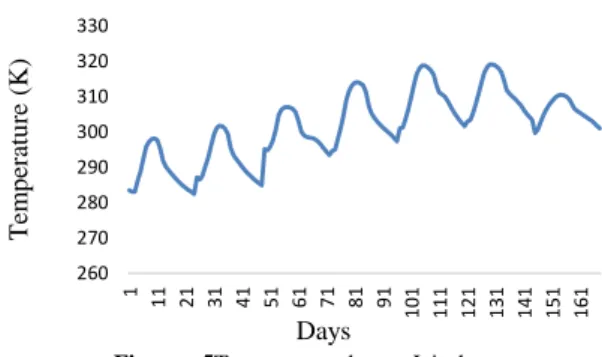
Temperature (T) is treated as physical phenomena indicate as hot and cold. Temperature is estimated with a thermometer adjusted in at least one-temperature scales. The most ordinarily utilized scales are the Celsius scale (meant °C). Here, temperature is taken as kelvin (K) and recorded at 2m above ground in this study. Temperature is significant in all fields of regular science, including material science, chemistry, Earth science, prescription, and biology, just as most aspects of everyday life. The sample of temperature at Jaisalmer is shown in figure 5.

0 10 20 30 40 50 60 70 80 1 9 ₁₇ ₂₅ ₃₃ ₄₁ ₄₉ ₅₇ ₆₅ ₇₃ ₈₁ ₈₉ ₉₇ 1 0 5 1 1 3 1 2 1 1 2 9 1 3 7 1 4 5 1 5 3 1 6 1 R el at iv r H u mi d it y ( %) Days 965 970 975 980 985 990 995 1000 1 ₁₀ ₁₉ ₂₈ ₃₇ ₄₆ ₅₅ ₆₄ ₇₃ ₈₂ ₉₁ 1 0 0 1 0 9 1 1 8 1 2 7 1 3 6 1 4 5 1 5 4 1 6 3 P re ss u re (h p a) Days 0 2 4 6 8 10 1 9 ₁₇ ₂₅ ₃₃ ₄₁ ₄₉ ₅₇ ₆₅ ₇₃ ₈₁ ₈₉ ₉₇ 1 0 5 1 1 3 1 2 1 1 2 9 1 3 7 1 4 5 1 5 3 1 6 1 W in d S p ee d (m /se c) Days

(4)

Figure : 5Temperature data at Jaisalmer

2.2.5 Wind Direction

Wind Direction (WD) is accounted for by the direction from which it starts. Generally, wind headings are estimated in units from 0° to 360°, however can on the other hand be indicated from - 180° to 180°. An assortment of instruments can be utilized to compute wind direction, for example, the wind vane and windsock. These such gadgets work by moving to limit air opposition. Here, wind direction is calculated as degree (deg) and estimated at 10m above ground in this study. The sample of wind direction at Jaisalmer is shown in figure 6.

Figure:6Wind direction data at Jaisalmer 3.METHODOLOGY

3.1 Multiple Linear Regression

To discover a single or multi-variate situation to fit a direct model, Linear Regression models have definite ways. Multiple linear regression is a kind of linear regression, which consists more than one dependent and independent variable. To describe the effect of selected independent variable on a subordinate variable, an analytical method i.e. Regression analysis is used. To assess the linear dependency of variable, linear regression is examined. The regression model clarifies the response of the undefined quantity (z) with the respect of known parameter and arbitrary noise and consider as a normally assign in both cases i.e. zero andconstant [14]. The generalized equation for linear regression model is shown in equation (1):

Where,

z = Dependent variable = Regression Coefficient = Independent variable

= Error accomplished due to regression The regression model gives the forecasted value ̂ is determined by equation (2):

̂ ∑

(2)

The most well-known strategy to calculate the regression coefficient ( ) is the reduction of the sum of square errors (SSE) as shown in equation (3):

∑

(3)

For wind speed prediction, one of the most utilized techniques is MLR. To match the design model and observed data, MLR technique is generally used to forecast in many research fields [15-16].

3.2 Calculation of the prediction performance After framing the multiple linear regression, their execution on the data index must be assessed. Distant error criteria have been introduced and utilized in the writing however, no single error criteria have been demonstrated to be the all-inclusive measures. Due to this, the pursuance of wind speed model become difficult to analyze. Hence, we have to assess the pursuance in view of numerous criteria.

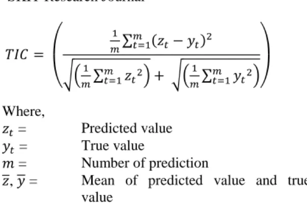
To analyze the prediction accuracy of various models, several estimation statistics can be utilized. These are Mean Absolute Percentage Error (MAPE), and Theil‘s Inequality Coefficient (TIC), Root Mean Squared Error (RMSE) and Correlation Coefficient (r) are utilized all the time to assess the pursuance of the prediction model [17]. These analytical quantities as shown below:

( ∑ ) (4) ( ∑ (| |) ) (5) ( (∑ ) √∑ ₎ (6) 260 270 280 290 300 310 320 330 1 ₁₁ ₂₁ ₃₁ ₄₁ ₅₁ ₆₁ ₇₁ ₈₁ ₉₁ 1 0 1 1 1 1 1 2 1 1 3 1 1 4 1 1 5 1 1 6 1 T em p era tu re (K) Days 0 50 100 150 200 250 300 350 400 1 9 ₁₇ ₂₅ ₃₃ ₄₁ ₄₉ ₅₇ ₆₅ ₇₃ ₈₁ ₈₉ ₉₇ 1 0 5 1 1 3 1 2 1 1 2 9 1 3 7 1 4 5 1 5 3 1 6 1 W in d Dire cti o n (d eg ) Days

(5)

( ∑ √( ∑ ) √( ∑ )₎ (7) Where, = Predicted value = True value = Number of prediction

, = Mean of predicted value and true value

RMSE is the standard deviation of the residuals and rely upon the size of the factors. Smaller MAPE shows the better prediction accuracy. Whereas TIC and MAPE are insensitive towards the size of the factors. Essentially, lower MAPE and TIC shows a superior prediction pursuance. TIC consists a value extending from 0 to 1. The predicted value shows the ideal fit to the true value when the TIC indicates zero.

Table :2 Analytical Pursuance for Ajmer Input

Combinations r RMSE MAPE TIC

T 0.545 1.892 0.647 6.27 p 0.578 1.788 0.622 5.53 RH 0.005 2.273 0.610 4.65 WD 0.341 2.166 0.593 4.938 T+p 0.596 1.759 0.636 5.90 p+RH 0.598 1.747 0.597 5.013 T+RH 0.771 1.495 0.573 5.483 T+WD 0.552 1.888 0.645 6.277 T+p+RH 0.737 1.513 0.582 5.388 P+RH+WD 0.620 1.712 0.593 5.209 RH+WD+T 0.764 1.496 0.582 5.439 WD+T+p 0.608 1.741 0.624 5.951 T+p+RH+WD 0.736 1.518 0.595 5.430

Table : 3 Analytical pursuance for banswara Input

T 0.452 1.762 0.476 2.943 p 0.647 1.457 0.392 2.436f RH 0.485 1.741 0.384 2.234 WD 0.53 1.911 0.551 3.163 T+p 0.647 1.458 0.378 2.340 p+RH 0.704 1.363 0.341 1.949 T+RH 0.735 1.486 0.364 2.175 T+WD 0.475 1.702 0.453 2.812 T+p+RH 0.747 1.464 0.344 2.128 p+RH+WD 0.712 1.344 0.324 1.929 RH+WD+T 0.744 1.453 0.364 2.187 WD+T+p 0.680 1.396 0.365 2.353 T+p+RH+WD 0.762 1.403 0.340 2.106 4. RESULTS

In this paper, we are using seven districts of Rajasthan and their analytical pursuance using Minitab 19 is shown in Table 2 to Table 8. For

forecasting the wind speed, as the number of input parameters are increasing, less error is obtained as shown in Table 2 to Table 8. MLR model, whose input parameters i.e. Temperature(T), Relative Humidity(RH) gives the best prediction results with fewer errors. Sometimes, in addition to Pressure (p), the obtained results got improved. However, by using the only RH, the forecasting of wind speed gives poor prediction.

Table :4Analytical Pursuance For Barmer

Input

Table :5Analytical pursuance for Bikaner

Input

Table: 6 Analytical Pursuance for Jaisalmer Input

T 0.504 1.765 0.357 2.277 p 0.672 1.472 0.324 2.063 RH 0.02 2.120 0.397 2.530 WD 0.215 1.994 0.403 2.583 T+p 0.673 1.482 0.317 2.033 p+RH 0.683 1.472 0.320 2.083 T+RH 0.646 1.613 0.363 2.369 T+WD 0.507 1.761 0.363 2.324 T+p+RH 0.685 1.467 0.323 2.097 p+RH+WD 0.685 0.072 0.323 2.107 RH+WD+T 0.646 0.249 0.362 2.352 WD+T+p 0.676 1.478 0.316 2.062 T+p+RH+WD 0.684 1.465 0.322 2.106

(6)

Input

T 0.597 1.829 0.455 3.486 p 0.661 1.665 0.432 3.388 RH 0.001 2.295 0.518 3.360 WD 0.117 2.246 0.538 3.462 T+p 0.674 1.645 0.428 3.400 p+RH 0.675 1.645 0.438 3.328 T+RH 0.815 1.552 0.448 3.144 T+WD 0.588 1.828 0.452 3.432 T+p+RH 0.750 1.524 0.422 3.150 p+RH+WD 0.671 1.644 0.435 3.264 RH+WD+T 0.771 1.443 0.398 2.864 WD+T+p 0.670 2.702 1.643 3.380 T+p+RH+WD 0.764 1.444 0.396 2.888

Table: 8 Analytical Pursuance for Sikar Input

T 0.243 1.194 0.508 3.383 p 0.115 1.223 0.501 3.284 RH 0.352 1.135 0.498 3.439 WD 0.084 1.536 0.475 2.901 T+p 0.341 1.138 0.491 3.319 p+RH 0.352 1.139 0.490 3.306 T+RH 0.299 1.184 0.507 3.306 T+WD 0.226 1.192 0.483 3.139 T+p+RH 0.338 1.141 0.491 3.374 P+RH+WD 0.354 1.149 0.466 3.032 RH+WD+T 0.290 1.175 0.473 2.919 WD+T+p 0.350 1.135 0.480 3.203 T+p+RH+WD 0.353 1.145 0.469 3.071 The MLR equation which is used to predict the wind speed based on the input parameters is shown in Table 9. These equations are obtained at the location of Jaisalmer.

Table: 9Mlr Equations for Jaisalmer

Parameters MLR Equations T R = -19.97+0.0791*T p R = 225.2-0.2244*p RH R = 3.308+0.0154*RH WD R = 2.592+0.00616*WD T+p R = 256.7-0.0161*T-0.2515*p p+RH R = 225.4-0.2251*p+0.01694*RH T+RH R = -28.35+0.1028*T+0.0525*RH T+WD R = -16.69+0.664*T+0.00283*WD T+p+RH R = 210.8+0.0074*T-0.2126*p+0.0195*RH P+RH+WD R = 215.1-0.2148*p+0.01482*RH+0.00119*W D RH+WD+T R = -29.11+0.0542*RH-0.00043*WD+0.1054*T WD+T+p R = 252.9+0.00203*WD-0.0231*T-0.2459*p T+p+RH+W D R = 224.7-0.0056*T-0.2228*p+0.0126*RH+0.00135*WD 5. CONCLUSION

MLR‘s focus is to build relationship in order to detect data patterns. The paper developed MLR techniques that can learn from past data and anticipate the future values using its learning. The highest reliable prediction of wind speed as for regression 0.815 and MAPE 0.4448 using MLR at Jodhpur with the help of T, and RH is from the analysis of seven meteorological stations. Wind speed measurement varies independently with regions and seasons. In the upcoming years, as the world is heading towards green energy, wind speed estimation can play a crucial role in deciding the potential for both wind energy and the weather geographical sites. To meet the overall energy requirement, it is required to develop highly accurate wind speed prediction method, So the future scope lies in applying the hybrid predicting models for predicting wind speed.

REFERENCES

[1] R. Foley, Aoife M., Paul G. Leahy, Antonino Marvuglia, and Eamon J. McKeogh. "Current methods and advances in forecasting of wind power generation." Renewable Energy 37, no. 1 (2012): 1-8.

[2] Rehman, Rehman, Shafiqur. "Wind energy resources assessment for Yanbo, Saudi Arabia." Energy Conversion and Management45, no. 13-14 (2004): 2019-2032.

[3] Rehman, Shafiqur, and Talal Omar Halawani. "Statistical characteristics of wind in Saudi Arabia." Renewable Energy 4, no. 8 (1994): 949-956. [4] Rehman, Shafiqur, T. O. Halawani, and Tahir Husain.

"Weibull parameters for wind speed distribution in Saudi Arabia." Solar Energy 53, no. 6 (1994): 473-479. [5] Hoppmann, Uwe, Stefan Koenig, Thorsten Tielkes, and

GerdMatschke. "A short-term strong wind prediction model for railway application: design and verification." Journal of wind engineering and industrial aerodynamics 90, no. 10 (2002): 1127-1134.

[6] Landberg, Lars. "Short-term prediction of the power production from wind farms." Journal of Wind Engineering and Industrial Aerodynamics 80, no. 1-2 (1999): 207-220.

[7] Riahy, G. H., and M. Abedi. "Short term wind speed forecasting for wind turbine applications using linear prediction method." Renewable energy 33, no. 1 (2008): 35-41.

[8] Catalina, Tiberiu, Vlad Iordache, and Bogdan Caracaleanu. "Multiple regression model for fast prediction of the heating energy demand." Energy and Buildings 57 (2013): 302-312.

[9] Jaffal, Issa, Christian Inard, and Christian Ghiaus. "Fast method to predict building heating demand based on the design of experiments." Energy and Buildings 41, no. 6 (2009): 669-677.

[10] Turalıoğlu, F. Sezer, AlperNuhoğlu, and HanefiBayraktar. "Impacts of some meteorological parameters on SO2 and TSP concentrations in Erzurum, Turkey." Chemosphere 59, no. 11 (2005): 1633-1642. [11] Abuella, Mohamed, and Badrul Chowdhury. "Solar

(7)

[12] Tar, Károly. "Some statistical characteristics of monthly average wind speed at various heights." Renewable and Sustainable Energy Reviews 12, no. 6 (2008): 1712-1724.

[13] Rajasthan Renewable Energy Corporation Limited

[online] Available:

http://energy.rajasthan.gov.in/content/raj/energy-department/rrecl/en/activities/wind.html, [Accessed: 2019]

[14] Agirre-Basurko, E., Gabriel Ibarra-Berastegi, and I. Madariaga. "Regression and multilayer perceptron-based models to forecast hourly O3 and NO2 levels in the Bilbao area." Environmental Modelling & Software 21, no. 4 (2006): 430-446.

[15] Khan, Zahid A., Irfan AnjumBadruddin, G. A. Quadir, and K. N. Seetharamu. "A quick and accurate estimation of heat losses from a cow." Biosystems engineering 93, no. 3 (2006): 313-323.

[16] Singh, Gyanendra. "Estimation of a mechanisation index and its impact on production and economic factors—A case study in India." Biosystems Engineering 93, no. 1 (2006): 99-106.

[17] Chatfield, Chris, and Andreas S. Weigend. "Time series prediction: Forecasting the future and understanding the past: Neil A. Gershenfeld and Andreas S. Weigend, 1994,'The future of time series', in: AS Weigend and NA Gershenfeld, eds, (Addison-Wesley,Reading, MA), 1-70." International Journal of forecasting 10, no. 1 (1994): 161-163.