Application of all-relevant feature selection for the failure analysis of parameter-induced simulation crashes in climate models

(1)

www.geosci-model-dev.net/9/1065/2016/ doi:10.5194/gmd-9-1065-2016

Application of all-relevant feature selection for the failure analysis of

parameter-induced simulation crashes in climate models

Wiesław Paja1, Mariusz Wrzesien2, Rafał Niemiec2, and Witold R. Rudnicki3,4

1_{Department of Computer Science, Faculty of Mathematics and Natural Sciences, University of Rzeszów, Rzeszów, Poland} 2_{Department of Artificial Intelligence and Expert Systems, Faculty of Applied Informatics, University of Information} Technology and Management, Rzeszów, Poland

3_{Institute of Informatics, University of Białystok, Białystok, Poland}

4_{Interdisciplinary Centre for Mathematical and Computational Modelling, University of Warsaw, Warsaw, Poland}

Correspondence to: Witold R. Rudnicki ([email protected])

Received: 9 May 2015 – Published in Geosci. Model Dev. Discuss.: 13 July 2015 Revised: 3 December 2015 – Accepted: 20 February 2016 – Published: 17 March 2016

Abstract. Climate models are extremely complex pieces of software. They reflect the best knowledge on the physical components of the climate; nevertheless, they contain sev-eral parameters, which are too weakly constrained by obser-vations, and can potentially lead to a simulation crashing. Re-cently a study by Lucas et al. (2013) has shown that machine learning methods can be used for predicting which combina-tions of parameters can lead to the simulation crashing and hence which processes described by these parameters need refined analyses. In the current study we reanalyse the data set used in this research using different methodology. We confirm the main conclusion of the original study concern-ing the suitability of machine learnconcern-ing for the prediction of crashes. We show that only three of the eight parameters in-dicated in the original study as relevant for prediction of the crash are indeed strongly relevant, three others are relevant but redundant and two are not relevant at all. We also show that the variance due to the split of data between training and validation sets has a large influence both on the accuracy of predictions and on the relative importance of variables; hence only a cross-validated approach can deliver a robust predic-tion of performance and relevance of variables.

1 Introduction

The development of realistic models of climate is one of the most important areas of research due to the dangers posed by global warming. It is by no means a trivial task since

it involves the parameterisation of many processes that are not directly solved within the model. It has been shown by Lucas et al. (2013) that certain combinations of these pa-rameters lead to failure of a model, despite each individual parameter having a reasonable value. Authors of this study performed 540 simulations with randomly varied combina-tions of 18 parameters of the Parallel Ocean Program (POP2) (Smith et al., 2010) module in the Community Climate Sys-tem Model Version 4 (CCSM4) (UCAR, 2010). About 10 % of these simulations crashed due to numerical instabilities. Then they applied machine learning methods to attribute fail-ures to the parameters of the model. To this end they used the support vector machine (SVM) (Vapnik, 1995) classification to quantify and predict the probability of failure as a function of the values of 18 POP2 parameters. The causes of the sim-ulation failures were determined through a global sensitivity analysis. Combinations of eight parameters related to ocean mixing and viscosity from three different POP2 parameter-isations were then determined as the major sources of the failures. These eight parameters were indicated as targets for more detailed research.

(2)

acute when a sample used for a machine-learning algorithm is small. In such a case random fluctuation may introduce spurious correlations within data, which can be utilised by the classification algorithm for model building. The appro-priate procedure should be applied to minimise the influence of such random correlations on the final results.

Lucas et al. (2013) have also analysed the impact of the de-cision variable that is used for the classification on the qual-ity of results. While the models were built as an ensemble of learners built on the bootstrap samples of the training set, the evaluation of the classification performance was based on a single split of data between training set and test set. This set-up was due to the construction of the study – simulations for the validation set were performed after the predictions had been made. While this is a very honest method for the veri-fication of the predictions, it precludes the estimation of the statistical uncertainty of the result. In particular, it is impos-sible to say whether the observed differences between clas-sification accuracy observed for different decision functions are significant or whether they arise due to statistical fluctu-ations.

The current study is devoted to the reanalysis of the data. It aims at minimising the influence of random fluctuations on the final results. Our aim was to establish all variables that truly contribute to the final result of the simulations, i.e. whether the simulation was finished successfully or whether it crashed. To this end we use contrast variables that carry no information on the decision variable and apply the Boruta algorithm for all-relevant feature selection and extensive Monte Carlo sampling. We also compare the quality of clas-sification for several subsets of variables used for prediction of simulation result, to perform a parallel check of relevance of variables.

2 Methods

Similarly to the original work, we rely on machine learning algorithms to identify parameters that critically influence the fate of the simulation. The fundamental idea is that, if the classification algorithm can predict result of the simulation, i.e. the successful completion of simulation or the crash, us-ing only the information on the values of certain combina-tions of selected parameters, then these parameters are in-deed responsible for the result. In the original paper the au-thors performed true prediction and achieved a high degree of accuracy, therefore showing the true predictive power of this approach. On the other hand, this set-up precludes estimation of statistical uncertainty for some of their findings. In partic-ular, the discussion of the prediction accuracy in Sects. 4.4 and 4.5 is based on a single split of data between training and test sets and ignores the possibility that effects may depend on the particular split.

In the current study we know all results beforehand; thus we are limited to virtual predictions only. In this approach we

split the entire data set into training and validation sets. We then build a model using the training set and check its qual-ity by performing virtual prediction on the validation set and comparing the predicted results with the true ones. One can take advantage of virtualisation to obtain information about the probability distribution of results. To this end one can per-form multiple virtual experiments, with different splits be-tween training and validation sets, and perform classification experiment on each of these splits. The results of individual trials will differ in most cases, allowing one to draw con-clusions not only about mean values but also about variance and even shape of probability distribution. Lucas et al. (2013) have used this approach for the sensitivity analysis, utilising ensembles of SVM (Vapnik, 1995) learners for classification. Each member of the ensemble was obtained using a different subsample of the training set. The classifier was then used for prediction of the simulation result for the validation set.

We used a different classification algorithm, namely the Random Forest (Breiman, 2001), and instead of the sensitiv-ity analysis we applied the all-relevant feature selection algo-rithm Boruta (Kursa et al., 2010). All computations were per-formed in the R environment for statistical modelling (R De-velopment Core Team, 2008), using the randomForest pack-age for classification (Liaw and Wiener, 2002) and the Boruta package for feature selection (Kursa and Rudnicki, 2010). In-terestingly, some of the authors of Lucas et al. (2013) have recently used Random Forest in their analysis of the results of the CAM5 model applied for study of Madden–Julian oscil-lation. It was applied to analyse the influence of the model parameters on selected diagnostic variables (Boyle et al., 2015).

Random Forest is an ensemble algorithm based on deci-sion trees. To ensure the low correlation between elementary learners, each tree is grown using a different random sub-sample of the original data set. Moreover, each split in the tree is built using only a random subset of the predictor vari-ables. The number of variables in this subset influences the balance between bias and variance for the training set. The default value for classification tasks is the square root of the total number of variables, and it is usually a very robust se-lection. Random Forest is a robust “off-the-shelf” algorithm that is easily applicable to various classification and regres-sion tasks. It has only few control parameters, and usually it does not need fine tuning for the particular problem under scrutiny. In many cases it has a performance comparable to or even better than state-of-the-art classifiers, and it rarely fails. A big advantage of the algorithm is that it estimates both the classification error and the importance of variables by inter-nal cross validation. To estimate the latter, it measures how much the accuracy of base learners is decreased when infor-mation about the variable in question is removed from the system.

(3)

46/45

S01_{: V}01₀₁_V01₀₂_{… V}01₁₈_C01₀₁_C01₀₂_{… C}01₁₈_:_D01_={F/S}

S02_{: V}02₀₁_V02₀₂_{… V}02₁₈_C02₀₁_C02₀₂_{… C}02₁₈_:_D02_={F/S} …

S92_{: V}92₀₁_V92₀₂_{… V}92₁₈_C92₀₁_C92₀₂_{… C}92₁₈_:_D92_={F/S}

Boruta()

ListOfImpVars : {V01,V02,V09,V13,V14,V16,C11}

540 objects 494 success 46 fail

10 sets

60 repeats

10 sets

10 sets + 46/45 46/45 46/45

46/44

+ 46/45 46/45 46/45 46/44

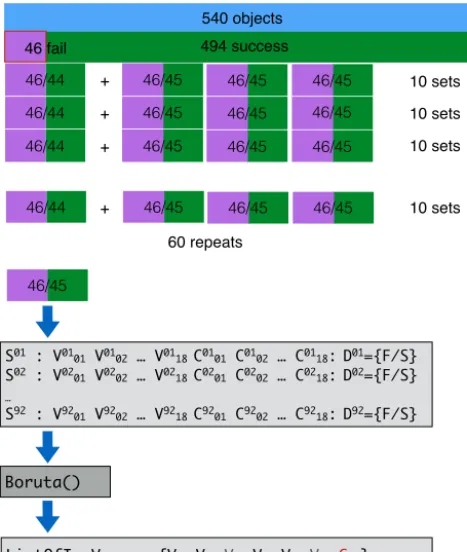
Figure 1. Protocol of the first test. The example list of important variables from a single Boruta run is shown. Core variables are high-lighted in boldface; the contrast variable is shown in red.

non-informative by design – the so-called contrast variables. It then compares the apparent importance of the original variables with that of the non-informative ones. It performs this multiple times using different realisations of the non-informative variables and performs a statistical test. The al-gorithm finds both strongly and weakly relevant variables. The notions of strong and weak relevance were introduced by Kohavi and John (1997) in the context of the ideal classi-fication algorithm. The features are strongly relevant when removing them from the description always results in de-creased classification accuracy. Features are weakly relevant when their removal in some cases may decrease classification accuracy. For a more detailed discussion of relevance and the Boruta algorithm see Kohavi and John (1997) and Rudnicki et al. (2015). This algorithm has been used in different fields, including bioinformatics, remote sensing, bacteriology and medicine (Aagaard et al., 2012; Ackerman et al., 2013; Bu-day et al., 2013; Duro et al., 2012; Herrera and Bazaga, 2013; Leutner et al., 2012; Ma et al., 2014; Menikarachchi et al., 2012; Saulnier et al., 2011; Strempel et al., 2013).

The climate simulation data set is highly biased towards successful completion of simulation. Only 46 cases out of 540 are failures. Such unbalanced data sets are often diffi-cult for classification, because the automatic selection of the majority class results in good, but useless, classification ac-curacy. In such a case no information is gained, and hence

30 repeats

329 S 31F

360 objects

Training set

494 S (success) 540 objects

46 F (failure)

165 S 15 F

180 objects

Test set Random

Forest ! model

AUC

Core+VTest

or Core-VTest

Variables

Figure 2. Protocol of the second test.

one cannot perform feature selection. In the first test of the current study this problem was avoided by application of the following protocol (see Fig. 1). Firstly 11 balanced subsam-ples of the training set were constructed; each subsample consisted of all objects from the minority class (failed sim-ulations) and 1 / 11 of the majority class (successful simula-tions). In order to check specificity of the feature selection, each data set was extended by contrast variables. To this end each original variable was duplicated, and its values were randomly permuted between all objects. In this way a set of

shadow variables that were non-informative by design was

added to the original variables. Then the feature selection procedure was performed on each subsample with the help of the all-relevant feature selection algorithm, implemented in the Boruta function of the Boruta package. The procedure was repeated 60 times. Altogether all-relevant feature selec-tion was performed 660 times. The number of times when the artificially constructed shadow variables were selected as important gives an estimate of the expected level of false dis-covery. The variables that were selected as important signifi-cantly more often than random were examined further, using a different test.

The second test probing the importance of variables was performed by analysing the influence of variables used for model building on the prediction quality. The first experi-ment revealed four variables that were classified as impor-tant by Boruta in all, or nearly all, of the 660 trials. These variables were considered to form a core variable set, and the model built using these variables was used as a reference. We examined whether removing one of the core variables or whether adding another variable respectively decreases or in-creases the classification quality measured by the area under the curve (AUC). The extension of the core test was exam-ined for three variables that were classified in the first test as important significantly more often than the randomised vari-ables.

(4)

● ● ● ● ● ● ● ● ● ● ● ● ● ● ● ● ● ● ● ● ●●●●●● ● ● ● ● ● ● ● ● ● ● ● ● ● ● ● ● ● ● ● ● ● ● ● ● ● ● ● ● ● ● ● ● ● ● ● ● ● ● ● ● ● ●

shadowMin V5 V17 shadowMean V13 shadowMax V4 V16 V9 V14 V1 V2

0 20 40 60 80 100 120 Attributes Impor tance

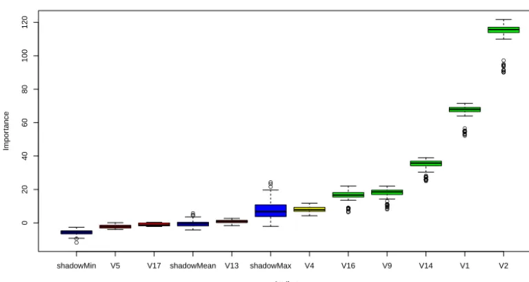
Figure 3. Summary of results of the Boruta run. Importance of the variables is shown. The variables are sorted by increasing importance. The variables coloured in green are those which were classified as relevant. Variables coloured in red are those which are irrelevant. The blue boxes correspond to minimal (sMin), median (sMed) and maximal (sMax) importance achieved in each run by contrast variables. One can observe a wide range of maximal-importance values that can be achieved by random variables. In particular in many iterations it can be higher than importance of truly relevant variables.

separately for the minority and majority class, so the number of minority class objects in each training set was 32 and in the validation set it was 14. The randomForest function from the identically named R package was used to perform clas-sification and error estimate. The procedure was repeated 30 times, and results of 30 repetitions were analysed.

The number of trees in the forest (parameter ntree both in randomForest and in Boruta functions) was set to 5000 both for feature selection with Boruta and classification with ran-domForest. In both cases the number of variables examined for each split was equal to the square root of the total number of variables. In our experience these settings are fairly robust; we have examined them internally over multiple data sets (Rudnicki et al., 2015). Moreover, we have checked whether they influence results in the initial trials. The number of trees used was 10 times higher than default, to assure that impor-tance estimate in Random Forest converge to their asymp-totic values; the number of trees for classification was the same for consistency.

3 Results and discussion

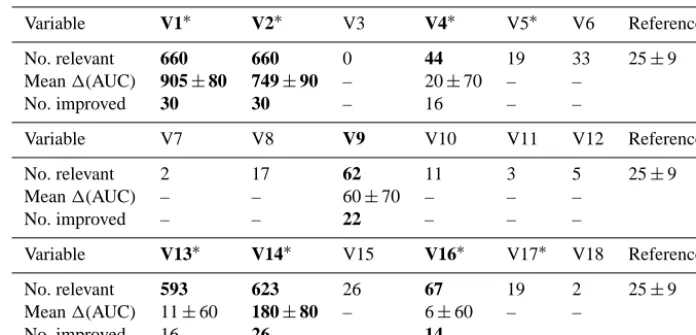
The summary of the results of the study is presented in Ta-ble 1. VariaTa-bles V1 and V2 were deemed important in all 660 cases. Variables V13 and V14 were deemed important in nearly all cases – 593 and 623 cases, respectively. All these variables were also indicated as most important by Lucas et al. (2013). However, the results do not agree so well for other variables. Lucas et al. (2013) indicated variables V4, V5, V16 and V17 as important, but their influence on the

fi-nal result was much weaker than that of the first group. In the current study variables V4 and V16 were deemed important by Boruta for 44 and 66 subsamples, respectively. In both cases the number is significantly higher than the average for the random variables, which was obtained as 25±9. On the other hand variables V5 and V17 were deemed important for 19 and 17 subsamples, respectively, and these numbers are lower than the average for random variables. Moreover, vari-able V9, which was not indicated as important by Lucas et al. (2013), was deemed important for 62 subsamples.

Hence the first experiment, which confirmed the impor-tance of variables V1 and V2, showed that imporimpor-tance of V13 and V14 is nearly universal; it also confirmed the weak importance of variables V4 and V16. On the other hand the importance of variables V5 and V17 was not confirmed with our method; instead variable V9 was found to be weakly im-portant. The example result of the Boruta run for an inter-esting sample is presented in Fig. 3. In this sample the im-portance was confirmed for variables V9 and V16, whereas variable V13 was deemed irrelevant. The importance of V4 was higher than that of the highest random variable, but only barely so, and hence the final decision of Boruta was “ten-tative”. One should note that the importance returned by Boruta is the averaged importance obtained from the un-derlying Random Forest algorithm. It is not directly inter-pretable in terms of the fraction of variance explained by a given variable.

(5)

Table 1. Summary of results. The variables indicated as important by Lucas et al. (2013) are marked with∗; the variables that were indicated

as important in the first test are highlighted in bold face.1(AUC) is given in 0.0001 units. Three values are reported; the number of times the

variable was deemed relevant, mean difference in AUC due to adding variable to set of variables and number of times AUC was improved by adding variable to set of variables. The first value is reported for all variables; the two others are reported only for the variables that were

deemed relevant significantly more often than randomised variables. The unit for1(AUC) is 0.0001.

Variable V1∗ V2∗ V3 V4∗ V5∗ V6 Reference

No. relevant 660 660 0 44 19 33 25±9

Mean1(AUC) 905±80 749±90 – 20±70 – –

No. improved 30 30 – 16 – –

Variable V7 V8 V9 V10 V11 V12 Reference

No. relevant 2 17 62 11 3 5 25±9

Mean1(AUC) – – 60±70 – – –

No. improved – – 22 – – –

Variable V13∗ V14∗ V15 V16∗ V17∗ V18 Reference

No. relevant 593 623 26 67 19 2 25±9

Mean1(AUC) 11±60 180±80 – 6±60 – –

No. improved 16 26 – 14 – –

strongly and weakly relevant variables. In the case of V1 and V2, removal of the variable from the core data set resulted in a dramatic drop of AUC, confirming that these variables are truly informative (see Table 1 and Fig. 2). In the case of V14 the difference in AUC – referenced further as1(AUC) – was smaller, but still statistically significant, whereas for V13 the

1(AUC) was much smaller than the standard deviation. Sim-ilarly, adding either of the three remaining variables – namely V4, V9 and V16 – to the core set leads to an increase of the AUC by an insignificant amount (see Table 1 and Fig. 4). Another auxiliary metric that can be used to evaluate the rel-evance of variables is the number of samples in which the AUC for the model containing the variable is higher than that for the model built without that variable. The results of this metric are consistent with results for the1(AUC) – it is 30 for both V1 and V2 and 26 for V14, and these are the only re-sults that are significantly different from random ones. There-fore one can conclude that only three variables – namely V1, V2 and V14 – are strongly relevant, whereas the remaining variables are weakly relevant.

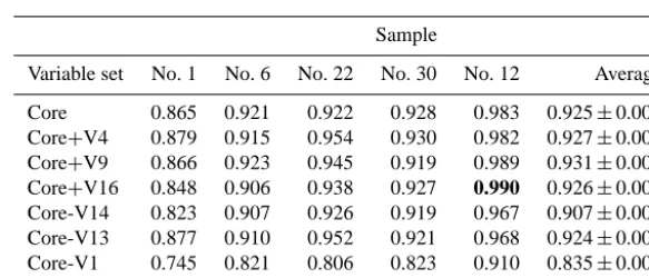
One should note that the results of the second test were highly variable and largely dependent on the split of data be-tween test and validation sets. This is illustrated in Fig. 5, and examples of the results from several samples are given in Ta-ble 2. The highest AUC obtained in the experiment was 0.990 for the model built using core variables and V16 in sample no. 12. In the same sample the AUC for the model built from core-V2 was 0.888. On the other hand for sample no. 1 the highest AUC was obtained for the model built on core+V9, and it was 0.879. The relative importance of variables also depends strongly on the test sample. For example adding variable V4 to the core set can improve AUC by as much as 0.032 (sample no. 22) or decrease it by 0.006 (sample no. 6).

●

C

C−13 C−14 C−2 C−1

C

C+9

C+16 C+4

C

0.75 0.80 0.85 0.90 0.95 1.00

Attributes

A

UR

OC

Figure 4. AUC obtained in simulation study grouped by subset of variables used for model building. The labels are coded in the

fol-lowing way: C – core set of variables{V1, V2, V13, V14}; C+X

– the core set was extended by adding variable VX, where X is one

of{4, 9, 16};C−X– the variable VX was removed from the core

set, with X= {1, 2, 13, 14}.

Similarly for V16 AUC can decrease by 0.016 (sample no. 6) or increase by 0.016 (sample no. 22). Most interestingly, re-moving variable V13, which was deemed relevant by Boruta in nearly 90% of samples, can either decrease the AUC by 0.011 (sample no. 6) or increase it by 0.030 (sample no. 22). These results show that one cannot rely on a single split be-tween the training set and test set for the estimate of influence of parameters, and that only the average over a sufficiently large number of alternative splits can give robust estimates.

(6)

●

● ●

●

● ●

●

1 2 3 4 5 6 7 8 9

10 11 12 13 14 15 16 17 18 19 20 21 22 23 24 25 26 27 28 29 30 0.75

0.80 0.85 0.90 0.95 1.00

Repeat

A

UR

OC

Figure 5. AUC obtained in simulation study grouped by split between training and validation set.

Table 2. Results of experiment 2. Average AUC obtained for all tested models, as well as examples for five interesting cases. No. 1 – the sample with the lowest AUC from core model; no. 12 the sample with the highest AUC obtained in the study; samples nos. 6, 22 and 30 – samples with core model close to the mean that show variance of AUC for other models. The highest AUC value obtained in the experiment is highlighted in boldface.

Sample

Variable set No. 1 No. 6 No. 22 No. 30 No. 12 Average

Core 0.865 0.921 0.922 0.928 0.983 0.925±0.006

Core+V4 0.879 0.915 0.954 0.930 0.982 0.927±0.007

Core+V9 0.866 0.923 0.945 0.919 0.989 0.931±0.006

Core+V16 0.848 0.906 0.938 0.927 0.990 0.926±0.007

Core-V14 0.823 0.907 0.926 0.919 0.967 0.907±0.007

Core-V13 0.877 0.910 0.952 0.921 0.968 0.924±0.006

Core-V1 0.745 0.821 0.806 0.823 0.910 0.835±0.007

Core-V2 0.808 0.808 0.825 0.840 0.888 0.850±0.009

nevertheless the value AUC=0.931 was not significantly higher than the value obtained for the simpler model built us-ing only three variables. The small differences in AUC arise due to small improvements for assigning the probability of failure of the simulation. Such improvement results in a small shift in the ranking from least probable to most probable to fail, without actually improving the error rate at the cost of including two more variables in the model.

A single run of the Boruta algorithm in the first test took 2 min on a server equipped with an Intel Xeon E5620 @ 2.4GHz CPU. The entire protocol took less than 24 h of sin-gle CPU core. The second test is far less computationally demanding. A single run of the randomForest function takes less than 20 s on the same CPU; therefore, computations for the entire protocol take less than 10 min. This effort is negli-gible in comparison with the time required to run 540 simu-lations of the climate model itself.

The results of the study are mostly in good agreement with the results of Lucas et al. (2013); however, importance of the variables is not identical. The most important difference is

(7)

mu-sical instruments (Kursa et al., 2009). The other differences are less important, since they involve variables with marginal relevance.

4 Conclusions

Our reanalysis of the results of 540 simulations is in general qualitative agreement with the results of Lucas et al. (2013). The results of the simulation can be predicted with fairly good accuracy using the machine learning approach, and the two different methods give very close results. The cross-validated AUC reported by Lucas et al. (2013) by ensemble of SVM classifiers was 0.93. In the current study the aver-age of the cross-validated AUC obtained for three strongly important variables was 0.924.

We have shown by cross validation that the AUC re-ported for the prediction experiment performed by Lucas et al. (2013) falls within the range of values that can be ex-pected in such a prediction; however, one should not assign any weight to the particular value obtained. If the split be-tween the training set and test set were set differently, the resulting AUC for prediction could be any number between 0.88 and 0.99.

The three most important conclusions for the climate mod-elling community are the following. Firstly, the efforts on im-proving the numerical stability of simulations should be con-centrated on three parameters of the CCSM4 parallel ocean model, namely vconst_corr, vconst_2 and bckgrnd_vdc1, which were earlier reported as most important by Lucas et al. (2013). The remaining parameters indicated as important in that study are either redundant or not relevant. Secondly, the machine learning methods in general and all-relevant fea-ture selection in particular are useful tools for analysis of in-fluence of simulation parameters on the final outcome. Fi-nally, application of machine learning should involve cross validation, and all important modelling steps should be in-cluded in the cross-validation loop.

Author contributions. Wiesław Paja performed most computations and drafted the first version of the manuscript; Mariusz Wrzesien and Rafał Niemiec performed computations and contributed to the writing. Witold R. Rudnicki designed the experiments and wrote the manuscript.

Edited by: S. Easterbrook

References

Aagaard, K., Riehle, K., Ma, J., Segata, N., Mistretta, T.-A., Coarfa, C., Raza, S., Rosenbaum, S., den Veyver, I., Milosavljevic, A., Gevers, D., Huttenhower, C., Petrosino, J., and Versalovic, J.: A Metagenomic Approach to Characterization of the Vagi-nal Microbiome Signature in Pregnancy, PLoS One, 7, e36466, doi:10.1371/journal.pone.0036466, 2012.

Ackerman, M. E., Crispin, M., Yu, X., Baruah, K., Boesch, A. W., Harvey, D. J., Dugast, A. S., Heizen, E. L., Ercan, A., Choi, I., Streeck, H., Nigrovic, P. A., Bailey-Kellogg, C., Scanlan, C., and Alter, G.: Natural variation in Fc glycosylation of HIV-specific antibodies impacts antiviral activity, J. Clin. Invest., 123, 2183– 2192, 2013.

Boyle, J. S., Klein, S. A., Lucas, D. D., Ma, H. Y., Tannahill, J., and Xie, S.: The parametric sensitivity of CAM5’s MJO, J. Geophys. Res.-Atmos., 120, 1424–1444, 2015.

Breiman, L.: Random forests, Mach. Learn., 5–32,

doi:10.1023/A:1010933404324, 2001.

Buday, B., Pach, F. P., Literati-Nagy, B., Vitai, M., Vecsei, Z., and Koranyi, L.: Serum osteocalcin is associated with improved metabolic state via adiponectin in females versus testosterone in males. Gender specific nature of the bone-energy homeostasis axis, Bone, 57, 98–104, doi:10.1016/j.bone.2013.07.018, 2013. Duro, D. C., Franklin, S. E., and Dubé, M. G.: Multi-scale

object-based image analysis and feature selection of multi-sensor earth observation imagery using random forests, Int. J. Remote Sens., 33, 4502–4526, 2012.

Herrera, C. M. and Bazaga, P.: Epigenetic correlates of plant phe-notypic plasticity: DNA methylation differs between prickly and nonprickly leaves in heterophyllous Ilex aquifolium (Aquifoli-aceae) trees, Bot. J. Linn. Soc., 171, 441–452, 2013.

Kohavi, R. and John, G. H.: Wrappers for feature subset selection, Artif. Intell., 97, 273–324, doi:10.1016/S0004-3702(97)00043-X, 1997.

Kursa, M., Rudnicki, W., Wieczorkowska, A., Kubera, E., and Kubik-Komar, A.: Musical instruments in random forest, in: Foundations of Intelligent Systems, LNCS 5722, 281–290, Springer Berlin Heidelberg, 2009.

Kursa, M. B. and Rudnicki, W. R.: Feature Selection with the Boruta Package, J. Stat. Softw., 36, 1–13, 2010.

Kursa, M. B., Jankowski, A., and Rudnicki, W. R.: Boruta – A sys-tem for feature selection, Fundam. Inform., 101, 271–285, 2010. Leutner, B. F., Reineking, B., Müller, J., Bachmann, M.,

Beierkuhn-lein, C., Dech, S., and Wegmann, M.: Modelling forest α

-diversity and floristic composition – on the added value of Li-DAR plus hyperspectral remote sensing, Remote Sens., 4, 2818– 2845, 2012.

Liaw, A. and Wiener, M.: Classification and Regression by random-Forest, R News, 2, 18—22, 2002.

Lucas, D. D., Klein, R., Tannahill, J., Ivanova, D., Brandon, S., Domyancic, D., and Zhang, Y.: Failure analysis of parameter-induced simulation crashes in climate models, Geosci. Model Dev., 6, 1157–1171, doi:10.5194/gmd-6-1157-2013, 2013. Ma, J., Prince, A. L., Bader, D., Hu, M., Ganu, R., Baquero, K.,

Blundell, P., Alan Harris, R., Frias, A. E., Grove, K. L., and Aa-gaard, K. M.: High-fat maternal diet during pregnancy persis-tently alters the offspring microbiome in a primate model, Nat. Commun., 5, 3889, doi:10.1038/ncomms4889, 2014.

Menikarachchi, L. C., Cawley, S., Hill, D. W., Hall, L. M., Hall, L., Lai, S., Wilder, J., and Grant, D. F.: MolFind: A Software Package Enabling HPLC/MS-Based Identification of Unknown Chemical Structures, Anal. Chem., 84, 9388–9394, doi:10.1021/ac302048x, 2012.

(8)

Vienna, Austria, ISBN 3-900051-07-0, available at: http://www. R-project.org (last access: 31 March 2015), 2008.

Rudnicki, W. R., Wrzesie´n, M., and Paja, W.: All Relevant Fea-ture Selection Methods and Applications, in: FeaFea-ture Selection for Data and Pattern Recognition, edited by: Sta´nczyk, U. and Lakhmi, C. J., 11–28, Springer-Verlag Berlin Heidelberg, Berlin, 2015.

Saulnier, D. M., Riehle, K., Mistretta, T.-A., Diaz, M.-A., Mandal, D., Raza, S., Weidler, E. M., Qin, X., Coarfa, C., Milosavljevic, A., Petrosino, J. F., Highlander, S., Gibbs, R., Lynch, S. V., Shul-man, R. J., and Versalovic, J.: Gastrointestinal microbiome sig-natures of pediatric patients with irritable bowel syndrome, Gas-troenterology, 141, 1782–91, doi:10.1053/j.gastro.2011.06.072, 2011.

Smith, R., Jones, P., Briegleb, B., Bryan, F., Danabasoglu, G., Dennis, J., Dukowicz, J., Eden, C., Fox-Kemper, B., Gent, P., Hecht, M., Jayne, S., Jochum, M., Large, W., Lindsay, K., Maltrud, M., Norton, N., Peacock, S., Vertenstein, M., and Yeager, S.: The Parallel Ocean Program (POP) reference manual: Ocean component of the Community Climate Sys-tem Model (CCSM), LAUR-10th–01, Los Alamos National Laboratory, available at: http://nldr.library.ucar.edu/repository/ collections/OSGC-000-000-000-954 (last access: 31 March 2015), 2010.

Strempel, S., Nendza, M., Scheringer, M., and Hungerbühler, K.: Using conditional inference trees and random forests to pre-dict the bioaccumulation potential of organic chemicals, Environ. Toxicol. Chem., 32, 1187–1195, 2013.

UCAR: The Community Climate System Model Version 4, avail-able at: http://www.cesm.ucar.edu/models/ccsm4.0/ (last access: 31 March 2015), 2010.