*
corresponding author
Analytical study of nano-bioconvective flow in a horizontal channel
using Adomian decomposition method
M. Kezzar a, b,M. R. Sarib, I. Tabetc and N. Nafird
a Mechanical engineering department, University of Skikda, El Hadaiek Road, B. O. 26, 21000 Skikda, Algeria.
b Laboratory of industrial mechanics, University Badji Mokhtar of Annaba, B. O. 12, 23000 Annaba, Algeria
c Physical engineering department, University of Skikda, El Hadaiek Road, B. O. 26, 21000 Skikda, Algeria
d Electrical engineering department, University of Skikda, El Hadaiek Road, B. O. 26, 21000 Skikda, Algeria
Article info:
Type: Research
Abstract
In this paper, the bioconvective nanofluid flow in a horizontal channel was considered. Using the appropriate similarity functions, the partial differential equations of the studied problem resulting from mathematical modeling are reduced to a set of non-linear differential equations. Thereafter, these equations are solved numerically using the fourth order Runge-Kutta method featuring shooting technique and analytically via the Adomian decomposition method (ADM). This study mainly focuses on the effects of several physical parameters such as Reynolds number (Re), thermal parameter (𝛿𝜃), microorganisms density
parameter (𝛿s) and nanoparticles concentration (𝛿) on the velocity, temperature,
nanoparticle volume fraction and density of motile microorganisms. It is also demonstrated that the analytical ADM results are in excellent agreement with the numerical solution and those reported in literature, thus justifying the robustness of the adopted Adomian Decomposition Method.
Received: 22/01/2018 Revised: 18/10/2018 Accepted: 20/10/2018 Online: 21/10/2018
Keywords:
Convection, Nanoparticles, Volume-fraction, Density of microorganisms, Adomian decomposition method.
Nomenclature
𝑎 and b Constants
𝑎0,.𝑎7 Constants
𝐴𝑛 Adomian polynomials
𝐶 Volumetric fraction of nanoparticles
𝐷𝑏 Brownian diffusion coefficient 𝐷𝑛 Diffusivity of microorganisms 𝐷𝑇 Thermo-phoretic diffusion
coefficient
𝜓 Stream function
𝐹 Dimensionless velocity
𝜃 Dimensionless temperature
Greek symbols
𝜂 Non-dimensional angle
𝛼 Thermal diffusivity
𝜁 Vorticity function
𝛾 Constant
𝛿
𝜃,
𝛿
,𝛿,𝛿𝑠 Constants 𝜌𝑓 Fluid density𝜌𝑠 Solid nanoparticles density 𝜙 Dimensionless nanoparticle
volume fraction
𝑃 Pressure
𝑁 density of motile microorganisms
𝑁𝑏 Brownian motion parameter 𝑁𝑡 Thermophoresis parameter 𝑃𝑟 Prandtl number
𝑃𝑒𝑏 Péclet number in bioconvection
application
𝑅𝑒 Reynolds number
ℓ Distance
𝐿𝑒 Lewis number 𝐿𝑖 Derivative operator 𝐿𝑖−1 Inverse derivative operator 𝑢, 𝑣 Velocity components along x-
and y-direction
𝑆𝑐 Schmidt number 𝑉, Velocity
𝑉̂ Velocity vector
𝑇 Temperature
𝑇0 Reference temperature
𝑊𝑐 Maximum cell swimming speed 𝜇𝑛𝑓 Dynamic viscosity of nanofluid 𝜈 Kinematic viscosity
𝜕 Derivative operator
Subscript
∎𝑛𝑓 Nanofluid ∎𝑓 Base fluid
∎𝑠 Solid nanoparticles
Abbreviation
𝑅𝐾4 Fourth order Runge-Kutta Method
𝐴𝐷𝑀 Adomian Decomposition Method
MLSM Modified Least Square Method
1. Introduction
Nowadays, it is well established that the nano-fluids play an important role in many domestic and industrial applications [1]. This novel category of fluids is created by the dispersion of the particles of nanometric size such as: Cu, Al2O3, SiC, ... in a base fluid like water.
Nano-fluids are very useful for thermal systems due to the higher thermal conductivity of solid nanoparticles when compared to that of the base fluid. The "nano-fluid" term was firstly proposed by Choi [2-3] since 1995. Subsequently, nano-fluids were characterized by several researchers experimentally [4-6] and theoretically [7-9]. Due to their superior thermal properties, Huminicet al. [10] have given an interesting review on the
Rayleigh number and the traditional thermal Rayleigh number. Mosayebidorcheh etal [20] studied the convective flow of a nano-fluid in a horizontal channel with the presence of gyrotactic microorganisms analytically. The mathematical model proposed by Nield and Kuznetsov was solved analytically by the Modified Least Square Method (MLSM). Particular attention was paid to the effects of various physical parameters on the evolution of velocity, temperature, nano-particles volume fraction and the density of motile microorganisms. Ramly et al. [21] studied the axisymmetric thermal radiative boundary layer flow of nanofluid over a stretched sheet. They investigated the effects of zero and nonzero fluxes on the thermal distribution and volumetric fraction of nanoparticles. Ramly et al. [22] also investigated the natural convection flow of nanofluid in Cheng-Minkowycz problem along a vertical plate. Rizwan Ul Haq et al. [23] investigated the fully developed squeezing flow of water functionalized magnetite nanoparticles between two parallel disks numerically. Three types of nanoparticles having better thermal conductivity: Magnetite (Fe3O4), Cobalt ferrite (CoFe2O4) and Mn–Zn ferrite (Mn– ZnFe2O4)
are added to the water base fluid.
In recent decades, several methods were developed in order to solve the nonlinear initial or boundary values problems analytically, such as the Adomian Decomposition Method (ADM), the Homotopy Analysis Method (HAM) and the Variational Iteration Method (VIM). The concept of decomposition method pioneered by George Adomian [24] has been efficiently used by several researchers [25-27]. Also, the Adomian decomposition method coupled with Padé approximants is employed by Noor [28-30] for the resolution of linear and nonlinear differential equations. Generally, Adomian Decomposition Method gives the solution in the form of a polynomial series and can be accurately applied without linearization, discretization or digital processing.
In the current study, Adomian decomposition method (ADM) is successfully applied to solve the nonlinear problem of nano bio-convective flow between two parallel plates. In fact, we were particularly interested on the evolution of velocity F (η), temperature θ (η), nano-particle volume fraction
(η) and density of motilemicroorganisms s (η) under the effects of several physical parameters such as thermal parameter (𝛿𝜃), nanoparticles concentration (𝛿),
microorganismas density parameter (𝛿𝑠) and
''𝑁𝑡/𝑁𝑏′' ratio.
2. Formulation of the problem
The heat transfer by convection in a fully developed flow of a nano-fluid between two parallel planar plates separated by a distance 2𝓵 was considered. Fig. 1 shows the geometry of the investigated flow.
Fig. 1. The geometry of the flow channel.
As drawn in Fig. 1, the "𝑂𝑦" axis is perpendicular to the walls, while the center of the channel is directed along the "𝑂𝑥" axis. The two walls (lower and upper) move (are stretched) at a speed of the form (𝑢 = 𝑎𝑥). The temperature at the walls is assumed to be constant. T1and T2
represent the temperatures of the lower and upper walls respectively. Moreover, the distribution of the nanoparticles at the base of the channel (lower wall) is assumed to have a constant C0 value. For the considered
nano-fluid, the basic fluid is water. A stable suspension of non-accumulating nanoparticles was considered.
Taking into account the above assumptions, the continuity equation, the momentum equation, the energy equation, the nanoparticle volume fraction equation and diffusion equation, as suggested by Kuznestov and Nield [31], can be expressed as follows :
∇ V = 0 (1)
𝜌𝑓(V ∇)V = −∇P + μ∇2V (2)
V∇𝑇 = 𝛼∇2𝑇 + 𝜏 [𝐷
𝐵∇𝑇∇𝐶 + (𝐷𝑇 𝑇 0
⁄ ) ∇𝑇∇𝑇] (3)
𝑢 = 𝑎𝑥
𝑢 = 𝑎𝑥 2ℓ
𝑧 𝑦
𝑥
𝑇2
(
V ∇)
C = 𝐷𝐵∇2C +(
𝐷𝑇⁄ )
𝑇0 ∇2𝑇 (4)𝛻. 𝑗 = 0, (5) where :
V is the velocity of the flow (function of u in the direction Ox and v in the direction Oy). The terms P and T represent the pressure and the temperature respectively. The constant C characterizes the volumetric fraction of the nanoparticles, DB is the Brownian diffusion
coefficient and DT is the thermo-phoretic
diffusion coefficient. T0 is a reference
temperature.
The density of a nanofluid is estimated by the parameter ρf and the dynamic viscosity of
nanofluid suspension is characterized by the term μ. The parameter τ characterizes the ratio ((ρc)p⁄(ρc)f) of thermal capacities of
nanoparticles and base fluid. The term α represents the thermal diffusivity of the nano-fluid.
Brownian motion is a random motion of particles suspended in the fluid as a consequence of quick atoms or molecules collision [32]. Thermophores refers to the transport of particles resulting from the temperature gradient [33]. j is another parameter defined according to the fluid convection, self-propelled swimming, and diffusion.
𝑗 = 𝑁𝑣 + 𝑁𝑣 − 𝐷𝑛𝛻𝑁,
(6)
Now, by introducing the parameters v̂ = (bWc
ΔC)∇C into the Eq. (6),we obtain:
𝑗 = 𝑁𝑣 + 𝑁(𝑏𝑊𝑐
𝛥𝐶)𝛻𝐶 − 𝐷𝑛𝛻𝑁
(7)
Where :
N : density of motile microorganisms.
v : velocity vector related to the cell swimming in nano-fluids.
Dn : diffusivity of microorganisms.
b and Wc : represent the constant of chemotaxis
and the maximum cell swimming speed respectively.
For a two dimensional flow, the Eq. (2) in Cartesian coordinates can be expressed as follows :
u∂u∂x+ v𝜕𝑢𝜕𝑦= −𝜌1
𝑓
𝜕𝑝 𝜕𝑥+ 𝜈 (
𝜕2𝑢
𝜕𝑥2+
𝜕2𝑢
𝜕𝑦2)
(8)
u∂v
∂x+ v ∂v ∂y= −
1 ρf
∂p ∂y+ ν(
∂2v ∂x2+
∂2u ∂y2) (9)
The parameter 𝜈 = 𝜇
𝜌𝑓 is the kinematic viscosity
of the nano-fluid.
Moreover, to simplify the Eqs. (1-4), the following equation is used:
𝜁 =
𝜕v𝜕𝑦
−
𝜕𝑢 𝜕𝑦= −∇
2
ψ
(9)Where
𝜁
is the vorticity functionTaking into account Eqs. (10, 1, 2, 3 and 4) become:
𝜕v 𝜕𝑥+
𝜕𝑢
𝜕𝑦= 0 (11)
𝑢𝜕𝜁
𝜕𝑥+ v 𝜕𝜁 𝜕𝑦= 𝛼 (
𝜕2𝜁
𝜕𝑥2+
𝜕2𝜁
𝜕𝑦2) (12)
𝑢𝜕𝑇 𝜕𝑥+ v
𝜕𝑇 𝜕𝑦= 𝛼 (
𝜕2𝑇 𝜕𝑥2+
𝜕2𝑇 𝜕𝑦2)
+ 𝜏 [𝐷𝐵∇𝑇 ( 𝜕𝐶 𝜕𝑥 𝜕𝑇 𝜕𝑥+ 𝜕𝐶 𝜕𝑦 𝜕𝑇 𝜕𝑦)
+ (𝐷𝑇 𝑇0
) ((𝜕𝑇 𝜕𝑥)
2 + (𝜕𝑇
𝜕𝑦) 2
)]
(13) 𝑢𝜕𝐶
𝜕𝑥+ v 𝜕𝐶
𝜕𝑦 = 𝐷𝐵( 𝜕2𝐶 𝜕𝑥2+
𝜕2𝐶 𝜕𝑦2) + (
𝐷𝑇 𝑇0 )𝜕 2𝑇 𝜕𝑥2 +𝜕 2𝑇 𝜕𝑦2 𝑢𝜕𝑁 𝜕𝑥 + v
𝜕𝑁 𝜕𝑦 +
𝜕
𝜕𝑦(𝑁𝑣 ) = 𝐷𝑁( 𝜕2𝑁 𝜕𝑥2)
With the relevant boundary conditions: 𝜕𝑢
𝜕𝑦= 0, v = 0 at y = 0
(16.a)
𝑢 = 𝑎𝑥, v = 0, 𝑇 = 𝑇2, 𝐷𝐵 𝑑𝐶 𝑑𝑦+ 𝐷𝑇
𝑇0
𝑑𝑇
𝑑𝑦 = 0 at y = ℓ
(16.b)
It is very important to normalize the equations of the investigated flow. To achieve this goal, we consider the dimensionless variables F(),θ(),
(
)
and 𝑆(𝜂) defined by:𝜂 = 𝑦⁄ ;ℓ
(𝑥, 𝑦) = 𝑎𝑥ℓ𝐹(𝜂) ; 𝜃(𝜂) = 𝑇 − 𝑇0
𝑇2 − 𝑇0 ;
(17)
𝑆(𝜂) = 𝑁 𝑁2
Considering terms of Eq. (17), Eqs. (12-15) become:
𝐹
′′′′+ 𝑅
𝑒(𝐹𝐹
′′′+ 4𝛼
2𝐹
′𝐹
′′) = 0
(18)(𝜃
′′+ 𝑅
𝑒𝑃
𝑟𝐹𝜃
′+ 𝑁
𝑏𝜃
′
′= 0
(19)
′′−
𝑁
𝑡𝑁
𝑏𝜃
′′
− 𝑅
𝑒
𝐿
𝑒𝐹
′= 0
(20)
𝑠
′′− 𝑃𝑒
𝑏(
′𝑠
′+ 𝑠
′′) + 𝑅
𝑒𝑆
𝑐𝐹𝑠
′= 0
(21) The Boundary conditions are:
At 𝜂 = −1𝜃(−1) = 𝛿𝜃, (−1) = 𝛿 and 𝑠 (−1) = 𝛿s
(22-a) At 𝜂 = 0𝐹(0) = 0
𝑎𝑛𝑑 𝐹 ′′(0) = 0 (22-b)
At 𝜂 = +1 𝐹(1) = 0, 𝐹 ′ (1) = 1, 𝜃(1) = 1, ′(1) + 𝛾𝜃 ′ (1) = 0
and𝑠 (1) = 1
(22-c)
The dimensionless numbers represented in Eqs. (18-21) are given as:
Reynolds number :𝑅𝑒= 𝑎.𝐿2
𝜈
Prandtlnumber :𝑃𝑟 = 𝜈 𝑎
Parameter of Brownian motion :𝑁𝑏 = 𝜏.𝐷𝐵.𝐶0
𝛼
Thermophoresis parameter: 𝑁𝑡 = ( 𝐷𝑇
𝑇0)
𝑇2−𝑇0
𝛼
Lewis number :𝐿𝑒= 𝜈 𝐷𝐵
Schmidt number :
𝑆
𝑐 = 𝜈𝐷𝑛
Péclet number in bioconvection application:
𝑃𝑒b=
𝑏Wc 𝐷𝑛
Constant 𝛾 = 𝑁𝑡
𝑁𝑏
3. Adomian decomposition method
In this section, we present the basic principle of Adomian decomposition method. Consider the following nonlinear differential equation:
𝐿(𝑦) + 𝑁(𝑦) = 𝑓(𝑡) (23) Where:
𝐿 =
𝑑𝑛∎𝑑𝑥𝑛
isthe n-order derivative operator, N is a
nonlinear operator and 𝑓 is a given function. Assume that L−1 is an inverse operator that represents n-fold integration for an n-th order of the derivative operator L. Applying the inverse operator 𝐋−1 to both sides of (Eq. (23)) yields:
{ L
−1= ∬ … . . ∫ ∎𝑑𝑥𝑛
𝐿−1𝐿(𝑦) = 𝐿−1𝑓 − 𝐿−1𝑁(𝑦)
(24)
As a result, we obtain:
𝑦 = 𝛽 + 𝐿−1𝑓 − 𝐿−1𝑁(𝑦) (25)
Where β is a constant determined from the boundary or initial conditions.
Now, based on the Adomian decomposition procedure, the solution y of the Eq. (23) can be constructed by a sum of components defined by the following infinite series:
𝑦 = ∑ 𝑦
𝑛 ∞𝑛=0
(26)
Also, the nonlinear term is given as follows:
𝑁𝑦 = ∑ 𝐴
𝑛(𝑦
0, 𝑦
1, … . , 𝑦
𝑛)
+∞𝑛=0
(27)
Where:
𝑦
0= 𝛽 + 𝐿
−1𝑓
,
𝑦
𝑛+1=
−𝐿
−1(𝐴
𝑛).
(28)
An′sare called the Adomian polynomials. The
recursive formula that defines the Adomian polynomials [24] is given as follows:
𝐴𝑛(𝑦0, 𝑦1, … . , 𝑦𝑛)
= 1 𝑛![
𝑑𝑛
𝑑𝜆𝑛[𝑁 (∑ 𝜆𝑖 ∞
𝑛=0
𝑦𝑖)]]
𝜆=0
,
𝑛 = 0,1,2, ….
(29)
𝑦 ≅ 𝑦
0+ 𝑦
1+ 𝑦
2+ 𝑦
3+ ⋯ + 𝑦
𝑛.
(30)
The Adomian decomposition method (ADM) is a powerful technique which provides efficient algorithms for several real applications in engineering and applied sciences. The main advantage of this method is to obtain the solution of both nonlinear initial value problems (IVPs) and boundary value problems (BVPs) as fast as convergent series with elegantly computable terms while it does not need linearization, discretization or any perturbation.
4. Implementing of ADM method
According to the principle of Adomian, Eqs. (18-21) can be written as:
L1F=-Re(FF'''+4α2F'F'')
(31)
𝐿2𝜃 = −𝑅𝑒𝑃𝑟𝐹𝜃′− 𝑁𝑏𝜃′∅′(32)
𝐿3∅ = − (𝑁𝑡⁄𝑁𝑏)𝜃′′− 𝑅𝑒𝐿𝑒𝑓∅′
(33)
L4s= +Peb(∅'s'+ s∅'')- (ReSc)fs'
(34)
Where differential operators (L1, L2, L3 and L4)
Are given by:L1= d4𝐹 dη4 ,L2=
d2𝜃 dη2 ,L3=
d2∅ dη2 and
L4= d2𝑆 dη2
The parameters L1, L2, L3 and L4 are the
differential operators. The inverses of these operators are expressed as:
{
𝐿1−1= ∭ ∫ 𝑭𝒅𝜼𝒅𝜼𝒅𝜼𝒅𝜼
𝜼
0
𝐿2−1= ∬ 𝜽𝒅𝜼𝒅𝜼 𝜼
0
𝐿3−1= ∬ ∅𝒅𝜼𝒅𝜼 𝜼
0
𝐿4−1= ∬ 𝒔𝒅𝜼𝒅𝜼
𝜼
0
(35)
By applying 𝐿𝑖-1(𝑖 = 1,2,3,4) to the Eqs. (27-28)
and considering boundary conditions (10), we get:
𝐹() = 𝐹(0) + 𝐹′(0)η +1 2𝐹
′′(0)η2+ 1
6𝐹
′′′(0)η3+ 𝐿
1−1(−𝑅𝑒(𝐹𝐹′′′+ 4𝛼2𝐹′𝐹′′))
(36) 𝜃() = 𝜃(0) + 𝜃′(0) η + 𝐿
2−1(−𝑅𝑒𝑃𝑟𝐹𝜃′
− 𝑁𝑏𝜃′∅′)
∅() = ∅(0) + ∅′(0) η + 𝐿2−1(− (𝑁𝑡⁄𝑁𝑏)𝜃′′
− 𝑅𝑒𝐿𝑒𝑓∅′)
𝑠() = 𝑠(0) + 𝑠′(0) η
+ 𝐿2−1(+𝑃𝑒𝑏(∅′𝑠′+ 𝑠∅′′)
− (𝑅𝑒𝑆𝑐)𝑓𝑠′)
Where:
NF = −Re(FF′′′+ 4α2F′F′′) (40)
Nθ = −RePrFθ′− Nbθ′∅′ (41)
N∅ = − (Nt⁄Nb)θ′′− ReLeF∅′ (42)
𝑁𝑠 = +𝑃𝑒𝑏(∅′𝑠′+ 𝑠∅′′) − (𝑅𝑒𝑆𝑐)𝐹𝑠′ (43)
The values of
F(0), F′(0) ,F′′(0), F′′′(0) ,θ(0), θ′(0) ,∅(0),
s(0) and s′(0) mainly depend on the boundary conditions. In fact, by applying the boundary conditions (8, 9) and considering: F′(0) = 𝑎0, F′′′(0) = 𝑎1, θ(0) = 𝑎2, θ′(0) =
𝑎3, ∅(0) = 𝑎4, ∅′(0) = 𝑎5, s(0) = 𝑎6, s′(0) =
𝑎7, we obtain:
𝐹(𝜂) = ∑ 𝐹
𝑛=
∞
𝑛=0
𝐹
0+ 𝐿
−1(𝑁𝐹)
(44)𝜃() = ∑ 𝜃𝑛= ∞
𝑛=0
𝜃0+ 𝐿−1(𝑁𝜃) (45)
∅() = ∑ ∅𝑛 = ∞
𝑛=0
∅0+ 𝐿−1(𝑁∅) (46)
𝑠(
) = ∑ 𝑠
𝑛=
∞
𝑛=0
𝑠
0+ 𝐿
−1(𝑁𝑠)
(47)Where
:
𝐹
0,
θ
0,
∅
0and
𝑠
0 are expressed as follows:F
0= 𝑎
0𝜂 + 𝑎
1𝜂
3
6
(48)
θ
0= 𝑎
2+ 𝑎
3𝜂
(49)
∅
0= 𝑎
4+ 𝑎
5𝜂
(50)
𝑠
0= 𝑎
6+ 𝑎
7𝜂
(51)
By the application of the algorithm (29), the polynomials (A0, A1, … … . . An) are expressed in
For velocity :
𝐴
0𝐹=
13𝑎1 2R
e𝜂3 (52-a)
𝐴
1𝐹=
− 112𝑎0𝑎1 2R
e2𝜂5− 11 1260𝑎1
2R
e2η7 (52-b)
For temperature
𝐴
0𝜃=
−𝑎3𝑎5Nb− 𝑎0𝑎3PrRe𝜂 − 1
6𝑎1𝑎3PrRe𝜂 3
(53-a)
A
θ1=
a3a52Nb2η+1
2a0a3a5LeNbReη
2
+3
2a0a3a5NbPrReη
2+1
2a0
2a
3Pr2Re2η3
+ 1
24a1a3a5LeNbReη
4+ 5
24a1a3a5NbPrReη
4
+1
8a0a1a3Pr
2R e2η5
− 1 2520a1
2a
3PrRe2η7+
1 144a1
2a
3Pr2Re2η
(53-b) For nanoparticle volume fraction:
𝐴
0−
𝑎0𝑎5Le
Re𝜂 −
16𝑎1𝑎5
Le
Re𝜂
3
(54-a)
𝐴
1=
𝑎3𝑎5Nt+ 1Nb𝑎0𝑎3NtPrRe𝜂 + 1
6Nb𝑎1𝑎3NtPrRe𝜂 3+1
2𝑎0 2𝑎
5Le2Re2𝜂3+ 1
8𝑎0𝑎1𝑎5Le 2R
e2𝜂5− 1 2520𝑎1
2𝑎
5LeRe2𝜂7+ 1
144𝑎1 2𝑎
5Le2Re2𝜂7 (54-b)
For density of motile microorganisms:
𝐴
0𝑠=
𝑎5𝑎7Pre− 𝑎0𝑎7ReSc𝜂 − 16𝑎1𝑎7ReSc𝜂
3
(55-a)
𝐴
1𝑠=
𝑎52𝑎7Pre2𝜂 − 𝑎0𝑎5𝑎6LePreRe𝜂 −3
2𝑎0𝑎5𝑎7LePreRe𝜂 2−3
2𝑎0𝑎5𝑎7PreReSc𝜂 2−
1
6𝑎1𝑎5𝑎6LePreRe𝜂 3+1
2𝑎0 2𝑎
7Re2Sc2𝜂3− 5
24𝑎1𝑎5𝑎7LePreRe𝜂 4− 5
24𝑎1𝑎5𝑎7PreReSc𝜂 4+
1
8𝑎0𝑎1𝑎7Re 2S
c2𝜂5− 1 2520𝑎1
2𝑎
7Re2Sc𝜂7+ 1
144𝑎1 2𝑎
7Re2Sc2𝛈𝟕 (55-b)
The application of Adomian Decomposition Method leads to the following solutions terms: For velocity :
𝐹
1=
12520𝑎1 2R
e
𝜂
7(56-a)
F2= −
1
36288𝑎0𝑎1
2R e2η9
− 1
907200𝑎1
3R e2η11
(56-b) For temperature
:
𝜃
1 = − 12𝑎3𝑎5Nb𝜂 2−1
6𝑎0𝑎3PrRe𝜂 3− 1
120𝑎1𝑎3PrRe𝛈
𝟓 (57-a)
θ
2=1 6a3a5
2N b2η3+
1
24a0a3a5LeNbReη
4
+1
8a0a3a5NbPrReη
4+ 1
40a0
2a
3Pr2Re2η5
+ 1
720a1a3a5LeNbReη
6+ 1
144a1a3a5NbPrReη
6
+ 1
336a0a1a3Pr
2R e2η7
− 1
181440a1
2a
3PrRe2η9+
1 10368a1
2a
3Pr2Re2η9
(57-b) For nanoparticle volume fraction:
∅1= −
1
6𝑎0𝑎5LeRe𝜂
3− 1
120𝑎1𝑎5LeRe𝜂
5
(58-a) ∅2=
1
2a3a5Ntη
2+ 1
6Nb
a0a3NtPrReη3
+ 1
120Nba1a3NtPrReη
5+ 1
40a0
2a
5Le2Re2η5
+ 1
336a0a1a5Le
2R e2η7
− 1
181440a1
2a
5LeRe2η9+
1 10368a1
2a
5Le2Re2η9
(58-b) For density of motile microorganisms
𝑠
1= 12𝑎5𝑎7Pre 𝜂 2−1
6𝑎0𝑎7Re
𝑆
𝑐𝜂 3− 1120𝑎1𝑎7Re
𝑆
𝑐 𝜂𝑠2
=1 6𝑎5
2𝑎
7Pre2𝜂3
−1
6𝑎0𝑎5𝑎6LePreRe𝜂
3
−1
8𝑎0𝑎5𝑎7LePreRe𝜂
4
−1
8𝑎0𝑎5𝑎7PreRe𝑆𝑐𝜂
4
− 1
120𝑎1𝑎5𝑎6LePreRe𝜂
5
+ 1 40𝑎0
2𝑎
7Re2𝑆𝑐2𝜂5
− 1
144𝑎1𝑎5𝑎7LePreRe𝜂
6
− 1
144𝑎1𝑎5𝑎7PreRe𝑆𝑐𝜂
6
+ 1
336𝑎0𝑎1𝑎7Re
2𝑆 𝑐2𝜂7
− 1
181440𝑎1
2𝑎
7Re2𝑆𝑐𝜂9
+ 1 10368𝑎1
2𝑎
7Re2𝑆𝑐2𝜂9
(59-b)
Finally, the approximate solutions for the studied problem are expressed as:
For velocity:
𝐹(𝜂) = 𝐹0+ 𝐹1+ ⋯ … … … . . +𝐹𝑛 (60)
For temperature:
𝜃(
𝜂)
=𝜃
0+𝜃
1+ ⋯ … … … . . +θn (61) For nanoparticle volume fraction: ∅(𝜂) = ∅0+ ∅1+ ⋯ … … … . . +∅𝑛 (62)
For density of motile microorganisms:
𝑠(
𝜂)
=𝑠
0+𝑠
1+ ⋯ … … … . . +𝑠
𝑛(63)
where: n is the iteration number.
The constants 𝑎0, 𝑎1, 𝑎2,𝑎3 ……., 𝑎7 can be
easily determined with the boundary conditions (Eqs. (22-a) - (22.c)).
5. Results and discussion
In this study, we were particularly interested in the evolution of velocity F(η), temperature θ(η), nano-particles volume fraction ∅(η) and density of motile microorganisms𝑠(η). The set of nonlinear differential equations (Eqs. (18-21)) with the boundary conditions (Eqs. (22)) are solved numerically and analytically. Numerically, the fourth-order Runge-Kutta
method was used. Analytically, the problem is treated via a powerful technique of computation called Adomian Decomposition Method. Figs. 2-4 show the effect of δθ parameter on the temperature, the nanoparticle volume fraction and the density of motile microorganisms respectively. It can be clearly seen that the δθ parameter has a significant effect on the behavior of temperature and nanoparticle volume fraction. As depicted in Fig. 2, the temperature increases with increasing δθ parameter. One can also observe that the δθ parameter has more effect on temperature at the lower wall (= −1) of the channel. In order to obtain a stable temperature profile along the channel, δθ parameter should be increased, which would result in higher temperature on the lower wall in comparison to the upper one. Furthermore, we can observe as displayed in Fig. 3 that the δθ parameter has more effect on the nanoparticle volume fraction at the lower wall (= +1). This means that increasing temperature of the channel wall leads to the concentration of the nanoparticles in the vicinity of the upper wall; and to reach a more stable profile, a higher δθ value is required. As drawn in Fig. 4, the behavior of motile microogranisms density s(η) as a function of δθ is approximately linear. The density s (η) increases as the δθ parameter increases.
when δs = 1, Nb= 0.2, Nt= 0.4, Pr = 1. Le= 2, Peb = 1, Sc= 3. δϕ = −0.5 and Re= 0.7
Fig. 5 shows the effect of δφ parameter on the behavior of nanoparticle volume fraction. We notice that the nanoparticles volume fraction appears as an increasing function of δφ.
Fig. 2. Effect of δθ parameter on the temperature evolution.
Fig. 3. Effect of δθ parameter on the evolution of
motile microorganisms density when δs = 1, Nb= 0.2, Nt= 0.4, Pr= 1. Le= 2, Peb= 1, Sc= 3. δϕ = −0.5 and Re= 0.7.
Fig. 4. Effect of δθ parameter on the evolution of nanoparticle volume fraction when: 𝛿𝑠 = 1, 𝑁𝑏= 0.2, 𝑁𝑡= 0.4, 𝑃𝑟= 1. L𝑒= 2, 𝑃𝑒𝑏= 1, 𝑆𝑐= 3. 𝛿𝜙 = −0.5 𝑎𝑛𝑑 𝑅𝑒= 0.7.
Fig. 5. Effect of δφ parameter on the evolution of nanoparticle volume fraction when δs = 1, Nb= 0.2, Nt= 0.4, Pr= 1. Le= 2, Peb = 1, Sc= 3. δθ = −0.5 and Re= 0.7.
Fig. 6. Effect of δs parameter on the evolution of motile microorganisms density when δθ = 0.2, Nb= 0.2, Nt= 0.4, Pr= 1. Le= 2, Peb = 1, Sc= 3. δϕ = −0.5 and Re= 0.7.
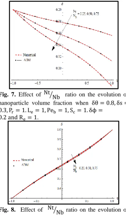
As can be seen from Fig. 7, the effect of the Nt
Nb
⁄ ratio is visibly greater with high values at the level of upper wall (= +1). By contrast, its effect on the density of microorganisms, as visualized in Fig. 8, is more pronounced along the axis of the channel (= 0). Furthermore, the Nt
Nb
augment of Reynolds number Re. In fact, the forced convection parameter Re has a drastic effect on the thermal behavior.
Consequently, with the increase of Reynolds number, the thermal layer becomes thin and concentrated near the wall. The greatest heat transfer rate is generally gained for the highest values of Reynolds number Re.
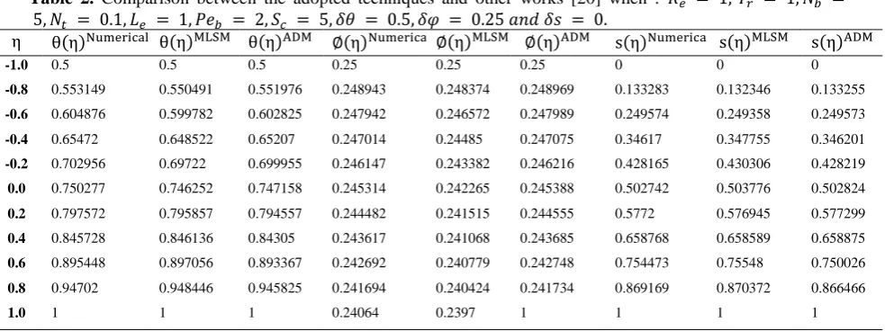
Table 1 represents a comparison between obtained numerical and analytical results. To highlight the effectiveness of the adopted analytical technique, a comparison with other works [16, 20] is reported in Figs. 10-11 and Table 2. Based on these comparisons, there is a clear evidence for a good agreement between analytical (ADM) and numerical (RK4) data, justifying the efficiency and the higher accuracy of the used Adomian decomposition method.
Fig. 7. Effect of Nt⁄Nb ratio on the evolution of nanoparticle volume fraction when δθ = 0.8, δs = 0.3, Pr= 1. Le= 1, Peb = 1, Sc= 1. δϕ =
0.2 and Re= 1.
Fig. 8. Effect of Nt⁄Nb ratio on the evolution of motile microorganisms density when δθ = 0.8, δs = 0.3, Pr= 1. Le = 1, Peb = 1, Sc= 1. δϕ =
0.2 and Re= 1.
Fig. 9. Heat transfer rate θ(−1) as a function of the
Nt Nb
⁄ ratio when δθ = 0.5, δs = 1, Pr= 1. Le= 1, Peb= 1, Sc= 1. δϕ = 0 and Re= 5
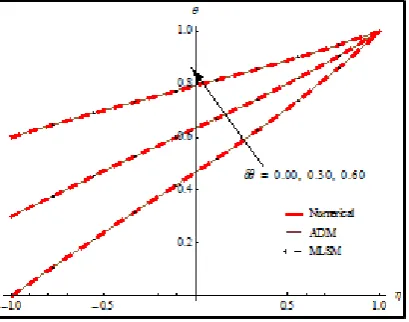
Fig. 10. Comparison between different results for temperature evolution when.δs = 1. Nt= 0.2. Pr= 3. Le= Peb = Sc = 1.δθ= 0.5.δϕ= 0. and Re= 5.
Fig. 11. Comparison between different results for nanoparticle volume fraction evolution when . 𝛿𝑠 = 1. 𝑁𝑡= 1. 𝑃𝑟= 1. 𝐿𝑒= 𝑃𝑒𝑏= 𝑆𝑐= 1. 𝛿𝜃 =
Table 1. Comparison of numerical and analytical results when :Nb= 0.2. Nt= 0.4. Pr = 1. Le= 5. δθ = 0.8, δ∅ = 0.2, δs = 0.1. and Re= 2.
𝐹(𝜂) 𝜃(𝜂) ∅(𝜂) 𝑠(𝜂)
𝜂 𝐹(𝜂)𝑅𝐾4 𝐹(𝜂)𝐴𝐷𝑀 𝜃(𝜂)𝑅𝐾4 𝜃(𝜂)𝐴𝐷𝑀 ∅(𝜂)𝑅𝐾4 ∅(𝜂)𝐴𝐷𝑀 𝑠(𝜂)𝑅𝐾4 𝑠(𝜂)𝐴𝐷𝑀 -1.00 0.000000 0.000000 0.8000 0.8000 0.20000 0.20000 0.100000 0.100000 -0.75 0.161449 0.161446 0.827456 0.827454 0.150759 0.150755 0.229558 0.229556 -0.50 0.183032 0.183035 0.853145 0.853142 0.119607 0.119603 0.341845 0.341843 -0.25 0.113997 0.113995 0.876783 0.876787 0.102894 0.102896 0.433844 0.433842 0.00 0.0000 0.0000 0.899207 0.899204 0.0924287 0.0924285 0.514763 0.514766 +0.25 −0.113997 −0.113994 0.921676 0.921673 0.0818686 0.0818684 0.596634 0.596637 +0.50 −0.183032 −0.183036 0.945487 0.945485 0.0647272 0.0647274 0.693681 0.693683 +0.75 −0.161449 −0.161443 0.971610 0.971614 0.0322616 0.0322617 0.824178 0.824176 +1.00 0.000000 0.000000 1.000000 1.000000 −0.0200213 −0.0200211 1.000000 1.000000
Table 2. Comparison between the adopted techniques and other works [20] when : 𝑅𝑒 = 1, 𝑃𝑟 = 1, 𝑁𝑏 = 5, 𝑁𝑡 = 0.1, 𝐿𝑒 = 1, 𝑃𝑒𝑏 = 2, 𝑆𝑐 = 5, 𝛿𝜃 = 0.5, 𝛿𝜑 = 0.25 𝑎𝑛𝑑 𝛿𝑠 = 0.
η θ(η)Numerical θ(η)MLSM θ(η)ADM ∅(η)Numerical ∅(η)MLSM ∅(η)ADM s(η)Numerical s(η)MLSM s(η)ADM
-1.0 0.5 0.5 0.5 0.25 0.25 0.25 0 0 0
-0.8 0.553149 0.550491 0.551976 0.248943 0.248374 0.248969 0.133283 0.132346 0.133255 -0.6 0.604876 0.599782 0.602825 0.247942 0.246572 0.247989 0.249574 0.249358 0.249573 -0.4 0.65472 0.648522 0.65207 0.247014 0.24485 0.247075 0.34617 0.347755 0.346201 -0.2 0.702956 0.69722 0.699955 0.246147 0.243382 0.246216 0.428165 0.430306 0.428219 0.0 0.750277 0.746252 0.747158 0.245314 0.242265 0.245388 0.502742 0.503776 0.502824 0.2 0.797572 0.795857 0.794557 0.244482 0.241515 0.244555 0.5772 0.576945 0.577299 0.4 0.845728 0.846136 0.84305 0.243617 0.241068 0.243685 0.658768 0.658589 0.658875 0.6 0.895448 0.897056 0.893367 0.242692 0.240779 0.242748 0.754473 0.75548 0.750026 0.8 0.94702 0.948446 0.945825 0.241694 0.240424 0.241734 0.869169 0.870372 0.866466
1.0 1 1 1 0.24064 0.2397 1 1 1 1
6. Conclusions
In this paper, the dynamic and thermal problems of a nano-fluid flow in a horizontal channel are considered. As a first step, the equations governing the problems are described in detail. In the current stuyd, the model proposed by Kuznestov and Nield [31] was adopted. Thereafter, the set of differential equations arising from mathematical modeling (velocity F(η), temperature θ(η), nanoparticles volume fraction 𝝋(η) and motile microorganisms density s(η)) are solved numerically and analytically by the Runge-Kutta method featuring technique and the Adomian decomposition method (ADM) respectively. The effects of various physical parameters, namely the thermal constant '' 𝛿𝜃 '', the concentration constant ''𝛿𝜑'' and ''𝑁𝑡/𝑁𝑏′'
ratio on the considered nano-fluid flow are visualized and discussed.
The main conclusions that may be drawn from this study are:
The thermal behavior and nanoparticles volume fraction are affected by the δθ constant particularly in the vicinity of the walls. In this region, the effect of δθ is more significant.
The nanoparticles volume fraction is an increasing function of δφ parameter.
The nanoparticles volume fraction is significantly affected by the δs constant, especially in the vicinity of the lower wall (= −1). However, for high δs values, the profile of nanoparticles volume fraction becomes stable.
Heat transfer rate θ(−1) raises with the increase of Reynolds number.
The obtained results highlight the robustness of the adopted analytical Adomian Decomposition Method (ADM) in comparison with numerical results and those of literature. Furthermore, the comparison reveals the applicability, reliability and simplicity of the used technique.
References
[1] R. Saidur, K. Y. Leong, Mohammad HaA. “A review on applications and challenges of nanofluids”, Renewable and sustainable energy reviews, Vol. 15, No. 3, pp. 1646-1668, (2011)
[2] S. U. S. Chol, J. A. Estman, “Enhancing thermal conductivity of fluids with nanoparticles”, ASME-Publications-Fed, Vol. 231, pp. 99-106, (1995).
[3] Stephen Choi, “US. Nanofluids: from vision to reality through research”, Journal of Heat transfer, Vol. 131, No. 3, p. 033106, (2009).
[4] S. M. S. Murshed, K. C. Leong, C. Yang, “Enhanced thermal conductivity of TiO2
-water based nanofluids”, International Journal of thermal sciences, Vol. 44, No. 4, pp. 367-373, (2005).
[5] Tae-Keun Hong, Ho-Soon Yang, C. J. Choi, “Study of the enhanced thermal conductivity of Fe nanofluids”, Journal of Applied Physics, Vol. 97, No. 6, p. 064311, (2005).
[6] XIE, Huaqing, Wang, Jinchang, Xi, Tonggeng, et al. “Thermal conductivity enhancement of suspensions containing nanosized alumina particles”, Journal of applied physics, Vol. 91, No. 7, pp. 4568-4572, (2002).
[7] Khalil Khanafer, Kambiz Vafai, , et Marilyn Lightstone, “Buoyancy-driven heat transfer enhancement in a two-dimensional enclosure utilizing nanofluids”, International journal of heat and mass transfer, Vol. 46, No. 19, pp. 3639-3653, (2003).
[8] M. Sheikholeslami, D. D. Ganji, “Heat transfer of Cu-water nanofluid flow between parallel plates”, Powder
Technology, Vol. 235, pp. 873-879, (2013).
[9] A. V. Kuznetsov, D. A. Nield, “Natural convective boundary-layer flow of a nanofluid past a vertical plate”, International Journal of Thermal Sciences, Vol. 49, No. 2, pp. 243-247, (2010).
[10] Gabriela Huminic, Angel Huminic, “Application of nanofluids in heat exchangers: a review”, Renewable and Sustainable Energy Reviews, Vol. 16, No. 8, pp. 5625-5638, (2012).
[11] Ping Cheng, W. J. Minkowycz, “Free convection about a vertical flat plate embedded in a porous medium with application to heat transfer from a dike”, Journal of Geophysical Research, Vol. 82, No. 14, pp. 2040-2044, (1977). [12] D. A. Nield, A. V. Kuznetsov, “The
Cheng–Minkowycz problem for natural convective boundary-layer flow in a porous medium saturated by a nanofluid”, International Journal of Heat and Mass Transfer, Vol. 52, No. 25-26, pp. 5792-5795, (2009).
[13] O. Pourmehran, M. Rahimi-Gorji, M. Gorji-Bandpy, ‘‘Analytical investigation of squeezing unsteady nanofluid flow between parallel plates by LSM and CM”. Alexandria Engineering Journal, Vol. 54, No. 1, pp. 17-26, (2015).
[14] Jacopo Buongiorno, “Convective transport in nanofluids”. Journal of heat transfer, Vol. 128, No. 3, pp. 240-250, (2006).
[15] Andrey V. Kuznetsov, “Nanofluid bioconvection in water-based suspensions containing nanoparticles and oxytactic microorganisms: oscillatory instability”, Nanoscale research letters, Vol. 6, No. 1, p. 100, (2011).
[17] Kalidas Das, Pinaki Ranjan Duari, Prabir Kumar Kundu, “Nanofluid bioconvection in presence of gyrotactic microorganisms and chemical reaction in a porous medium”, Journal of Mechanical Science and Technology, Vol. 29, No. 11, pp. 4841-4849, (2015).
[18] S. Ghorai, N. A. Hill, “Development and stability of gyrotactic plumes in bioconvection”, Journal of Fluid Mechanics, Vol. 400, pp. 1-31, (1999). [19] A. V. Kuznetsov, “New developments in
bioconvection in porous media: bioconvection plumes, bio-thermal convection, and effects of vertical vibration. In : Emerging Topics in Heat and Mass Transfer in Porous Media”. Springer, Dordrecht, pp. 181-217, (2008). [20] S. Mosayebidorcheh, M. A. Tahavori, T.
Mosayebidorcheh, “Analysis of nano-bioconvection flow containing both nanoparticles and gyrotactic microorganisms in a horizontal channel using modified least square method (MLSM)”, Journal of Molecular Liquids, Vol. 227, pp. 356-365, (2017).
[21] N. A. Ramly, S. Sivasankaran, N. F. M. Noor, “Zero and nonzero normal fluxes of thermal radiative boundary layer flow of nanofluid over a radially stretched surface”, Scientia Iranica, Vol. 24, No. 6, pp. 2895-2903, (2017).
[22] N. A. Ramly, S. Sivasankaran, N. F. M. Noor, “Numerical solution of Cheng-Minkowycz natural convection nanofluid flow with zero flux”, In: AIP Conference Proceedings. AIP Publishing, p. 030020, (2016).
[23] Rizwan Ul Haq, N. F. Noor, Z. H. Khan, “Numerical simulation of water based magnetite nanoparticles between two parallel disks, Advanced Powder Technology, Vol. 27, No. 4, pp. 1568-1575, (2016).
[24] G. Adomian, “Solving Frontier Problems of Physics: The Decomposition Method”, Klumer, Boston, (1994). [25] Mohammed Sari, Mohamed Rafik
Kezzar, Rachid Adjabi, “A Comparison of Adomian and Generalized Adomian
Methods in Solving the Nonlinear Problem of Flow in Convergent-Divergent Channels”, Applied Mathematical Sciences, Vol. 8, No. 7, pp. 321-336, (2014).
[26] Mohamed Kezzar, Mohamed Rafik Sari, “Application of the generalized decomposition method for solving the nonlinear problem of Jeffery–Hamel flow”, Computational Mathematics and Modeling, Vol. 26, No. 2, pp. 284-297, (2015).
[27] Mohamed Kezzar, Mohamed Rafik Sari, “Series Solution of Nanofluid Flow and Heat Transfer Between Stretchable/ Shrinkable Inclined Walls”, International Journal of Applied and Computational Mathematics, Vol. 3, No. 3, pp. 2231-2255, (2017).
[28] Noor Fadiya Mohd Noor, Muhaimin Ismoen, Ishak Hashim, “Heat-transfer analysis of mhd flow due to a permeable shrinking sheet embedded in a porous medium with internal heat generation”, Journal of Porous Media, Vol. 13, No. 9, pp. 847-854, (2010). [29] N. F. M. Noor, Ishak Hashim, “MHD
viscous flow over a linearly stretching sheet embedded in a non-Darcian porous medium”, J. Porous Media, Vol. 13, No. 4, pp. 349-355, (2010).
[30] N. F. M. Noor, S. Awang Kechil, Ishak Hashim, “Simple non-perturbative solution for MHD viscous flow due to a shrinking sheet”, Communications in Nonlinear Science and Numerical Simulation, Vol. 15, No. 2, pp. 144-148, (2010).
[31] A. V. Kuznetsov, D. A. Nield, “The Cheng–Minkowycz problem for natural convective boundary layer flow in a porous medium saturated by a nanofluid: a revised model”, International Journal of Heat and Mass Transfer, Vol. 65, pp. 682-685, (2013).
[33] Daniele, Vigolo, Roberto, Rusconi, Howard A. Stone, “Thermophoresis: microfluidics characterization and separation”, Soft Matter, Vol. 6, No. 15, pp. 3489-3493, (2010).
How to cite this paper:
M. Kezzar, M. R. Sari, I. Tabet, N. Nafir, “ Analytical study of Nano-bioconvective flow in a horizontal channel using adomian decomposition method”, Journal of Computational and Applied Research in Mechanical Engineering, Vol. 9, No. 2, pp. 245-258, (2019).