Effect of welding parameters on pitting corrosion rate of pulsed current micro plasma arc welded AISI 304L sheets in 1N HCl

(1)

1 *_{Corresponding author}

Effect of welding parameters on pitting corrosion rate of pulsed

current micro plasma arc welded AISI 304L sheets in 1N HCl

Kondapalli Siva Prasada*, Chalamalasetti Srinivasa Raob and Damera Nageswara Raoc

a

Assistant Professor, Department of Mechanical Engineering, Anil Neerukonda Institute of Technology & Sciences , Visakhapatnam, India

b

Associate Professor, Department of Mechanical Engineering, AU College of Engineering, Andhra University, Visakhapatnam, India

c

Vice Chancellor, Centurion University of Technology & Management, Odisha, India

Article info: Abstract

Austenitic stainless steel sheets have gained wide acceptance in the fabrication of components, which require high temperature resistance and corrosion resistance such as metal bellows used in expansion joints in aircraft, aerospace and petroleum industries. In the case of single pass welding of thinner sections of this alloy, Pulsed Current Micro Plasma Arc Welding (PCMPAW) has been found beneficial due to its advantages over the conventional continuous current process. This paper highlighted development of empirical mathematical equations using multiple regression analysis, correlating various process parameters to pitting corrosion rates in PCMPAW of AISI 304L sheets in 1 Normal HCl. The experiments were conducted based on a five factor, five level central composite rotatable design matrix. The model adequacy was checked by Analysis of Variance (ANOVA). The main effects and interaction effects of the welding process parameters on pitting corrosion rates of the welded joints were studied using surface and contour plots. From the contour plots, it was understood that peak current was the most influencing factor on the pitting corrosion rate. The optimum pitting corrosion rate was achieved at peak current of 6 Amperes, base current of 4 Amperes, pulse rate of 40 pulses/second and pulse width of 50 % .

Received: 10/08/2012 Accepted: 08/04/2013 Online: 11/09/2013

Keywords:

AISI 304L, Pulsed current,

Micro plasma arc welding, Pitting corrosion.

1.

Introduction

AISI 304L is an austenitic stainless steel with excellent strength and good ductility at high temperature. Its typical applications include aero-engine hot section components, miscellaneous hardware, tooling and liquid rocket components involving cryogenic

(2)

JCARME Kondapalli Siva Prasad, et al. ̀Vol. 3, No. 1, Autumn 2013

2

bellows and diaphragms which require high strength and toughness. PAW is conveniently carried out using one of the two different current modes, namely a Continuous Current (CC) mode or a Pulsed Current (PC) mode. Pulsed current MPAW involves cycling the welding current at the selected regular frequency. The maximum current is selected to give adequate penetration and bead contour while the minimum is set at a level sufficient for maintaining a stable arc [1, 2], which permits arc energy to be used effectively for fusing a spot of controlled dimensions in a short time, producing the weld as a series of overlapping nuggets. In pulsed current welding, the heat required for melting the base material is supplied only during the peak current pulses, allowing for the heat to dissipate into the base material leading to narrower Heat Affected Zone (HAZ). The advantages include improved bead contours, greater tolerance to heat sink variations, lower heat input requirements, reduced residual stresses and distortion, refinement of fusion zone microstructure and reduced width of HAZ. Based on the worked published as [3- 8] , four independent parameters that influence the process are peak current, back current, pulse rate and pulse width.

Neusa Alonso-Falleiros et al. [9] examined effect of surface finish of two AISI 304L (UNS S30403) stainless steels on the corrosion potential (Ecorr) in 3.5% NaCl aqueous solution. B. Tsaneva et al. [10] studied influence of temperature (0-800C) on corrosion - electrochemical parameters of austenitic Cr/4Mn/5N and Cr/8Mn/2N stainless steels in 3.5% NaCl by cyclic potentiodynamic method. P. Fauvet et al. [11] analyzed various austenitic stainless steel types 304L, 316L and 310Nb and noticed that austentic stainless steels were largely used as structural materials for the equipment handling nitric acid media in reprocessing plants. D. J. Lee et al. [12] investigated effect of pitting corrosion behavior on welded joints of AISI 304L austenitic stainless steel by the flux-cored arc welding process. Effect of welding parameters (power input, weld geometry, welding speed and post-weld heat treatment) on the corrosion behavior

of austenitic stainless steel in chloride medium was investigated by Ayo Samuel Afolabi [13]. Yunan Prawoto et al. [14] carried out a corrosion test to study performance of a duplex stainless steel alloy under several conditions using various pH and chloride concentrations at different temperatures. Girija Suresh et al. [15] conducted Electrochemical Noise (EN) monitoring of 304L stainless steel (SS) and sensitized 304 SS in 3N nitric acid and nuclear near-high level waste solution using a three nominally identical electrode configuration under open circuit conditions. Y. Ait Albrimi et al. [16] investigated electrochemical behavior of AISI 316 austenitic stainless steel in deaerated hydrochloric and sulphuric acid solutions using open-circuit potential, cyclic voltammetric and chronoamperometric techniques. Md. Asaduzzaman et al. [17] investigated the pitting corrosion behavior of the austenitic stainless steel in aqueous chloride solution using electrochemical technique. Moreover, M. Saadawy [18] studied effect of chloride ion addition on the corrosion of stainless steel 304 in Na2SO4 solution under constant ionic strength conditions at 30°C using potential-time and potentiodynamic polarization techniques.

In this investigation, the experiments in the design of experimental concept were used for developing mathematical models to predict such variables. Many works have been reported in the past for predicting bead geometry, heat-affected zone, bead volume, etc. using mathematical models for various welding processes [19- 21]. Usually, the desired welding process parameters are determined based on the experience of skilled workers or from the data available in the handbook. This does not ensure formation of optimal or near-optimal weld pool geometry [22]. It has been proven by several researchers that efficient use of statistical design of experimental techniques and other optimization tools can impart scientific approach in a welding procedure [23, 24]. These techniques can be used to achieve optimal or near-optimal bead geometry from the selected process parameters.

(3)

JCARME Effect of welding parameters on . . . Vol. 3, No. 1, Autumn 2013

3 Taguchi methods could be effective only when

the welding process was set near the optimal conditions or in a stable operating range [25]; but, near-optimal conditions could not be easily determined through full-factorial experiments when the number of experiments and levels of variables were increased. Also, the method of steepest ascent based upon derivatives could lead to incorrect direction of search due to non-linear characteristics of the welding process. The main objective of the present work was to study the main and interaction effects of PCMPAW parameters on pitting corrosion rate in 1N HCl medium.

2. Experimental procedure

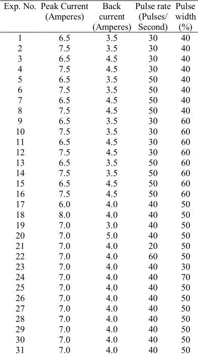
Austenitic stainless steel (AISI 304L) sheets of 100 x 150 x 0.25 mm were welded autogenously with square butt joint without edge preparation. The chemical composition of SS304L stainless steel sheet is given in Table 1. High purity argon gas (99.99%) was used as a shielding gas and a trailing gas right after the welding to prevent absorption of oxygen and nitrogen from the atmosphere. Welding was carried out under the welding conditions presented in Table 2. From the literature, four important factors of pulsed current MPAW as presented in Table 3 were chosen. A large number of trail experiments were carried out using 0.25 mm thick AISI 304L sheets to find out the feasible working limits of pulsed current MPAW process parameters. Due to the wide range of factors, it was decided to use a four factor, five level, rotatable central composite design matrix to perform a number of experiments for the purpose of this investigation. Table 4 indicates 31 sets of coded conditions used for forming the design matrix. The first sixteen experimental conditions (rows) were formed for main effects. The next eight experimental conditions were called corner points and the last seven ones were known as

center points. The method of designing such a matrix has been mentioned in [26, 27]. For the convenience of recording and processing the experimental data, upper and lower levels of the factors were coded as +2 and -2, respectively, and the coded values of any intermediate levels was calculated using Eq. (1) [28].

Xi = 2[2X-(Xmax + Xmin)] / (Xmax – Xmin) (1) where Xi is the required coded value of a parameter X. X is any value of the parameter from Xmin to Xmax, where Xmin is lower limit of the parameter and Xmax is upper limit of the parameter.

The welded joints were sliced at the mid-section to prepare pitting corrosions' test specimens. For pitting corrosion test, specimens of 50× 50 mm (width and length) were prepared to ensure exposure of 12 mm diameter circular area in the weld region to the electrolyte. The rest of the area was covered with an acid resistant lacquer. The specimen size and dimensions are given in Fig. 1. The specimen surface was polished strictly following metallographic procedures. The polarisation studies of the welds were carried out in 1 N HCl solution. Analar grade chemicals and double distilled water were used for preparation of the electrolyte. The schematic circuit diagram of the potentiodynamic polarization set up is shown in Fig. 2. A potentiostat (Make: AUTOLAB /PGSTAT12) was used for this study in conjunction with an ASTM standard cell and personal computer. The experiments were performed in 2 h duration, each at the scan rate of 1 millivolts/mm. The pitting corrosion rate was calculated by polarizing the specimen anodically and cathodically and by extrapolating the Tafel regions of anodic and cathodic curves to the corrosion potential. The experimentally evaluated results are presented in Table 4.

Table 1. Chemical composition of AISI 304L (weight %).

C Si Mn P S Cr Ni Mo Ti N

(4)

JCARME Kondapalli Siva Prasad, et al. Vol. 3, No. 1, Autumn 2013

4

Table 2 .Welding conditions.

Power source Secheron Micro Plasma Arc Welding Machine (Model:

PLASMAFIX 50E)

Polarity DCEN

Mode of operation Pulse mode

Electrode 2% thoriated tungsten electrode

Electrode Diameter 1mm

Plasma gas Argon & Hydrogen

Plasma gas flow rate 6 Lpm

Shielding gas Argon

Shielding gas flow rate 0.4 Lpm

Purging gas Argon

Purging gas flow rate 0.4 Lpm

Copper Nozzle diameter 1mm

Nozzle to plate distance 1mm

Welding speed 260mm/min

Torch Position Vertical

Operation type Automatic

Table 3. Important factors and their levels.

Levels

Serial No. Input Factor Units -2 -1 0 +1 +2

1 Peak Current Amperes 6 6.5 7 7.5 8

2 Back Current Amperes 3 3.5 4 4.5 5

3 Pulse rate Pulses/Second 20 30 40 50 60

4 Pulse width % 30 40 50 60 70

Fig. 1. Dimensions of corrosion test specimen.

Fig. 2. Block diagram for the experimental set up.

A- Reference Electrode B- Auxiliary Electrode (Platinum) C-Working Electrode (AISI 304L) D- Auto lab/PGTAT12

(5)

5

Table 4. Typical design matrix.

Exp. No. Peak Current (Amperes)

Back current (Amperes)

Pulse rate (Pulses/ Second)

Pulse width (%)

1 6.5 3.5 30 40

2 7.5 3.5 30 40

3 6.5 4.5 30 40

4 7.5 4.5 30 40

5 6.5 3.5 50 40

6 7.5 3.5 50 40

7 6.5 4.5 50 40

8 7.5 4.5 50 40

9 6.5 3.5 30 60

10 7.5 3.5 30 60

11 6.5 4.5 30 60

12 7.5 4.5 30 60

13 6.5 3.5 50 60

14 7.5 3.5 50 60

15 6.5 4.5 50 60

16 7.5 4.5 50 60

17 6.0 4.0 40 50

18 8.0 4.0 40 50

19 7.0 3.0 40 50

20 7.0 5.0 40 50

21 7.0 4.0 20 50

22 7.0 4.0 60 50

23 7.0 4.0 40 30

24 7.0 4.0 40 70

25 7.0 4.0 40 50

26 7.0 4.0 40 50

27 7.0 4.0 40 50

28 7.0 4.0 40 50

29 7.0 4.0 40 50

30 7.0 4.0 40 50

31 7.0 4.0 40 50

Amperes, back current of 4.5 Amperes,

pulse rate of 30 pulses/second and pulse

width of 40 %.

3. Experimental results

The measured pitting corrosion rate for all

the 31 samples as per typical design matrix

is presented in Table 5.

According to the conducted experiments, it

could be understood that the minimum

pitting corrosion rate of 0.54929 mm/year

was obtained for the peak current of 6.5.

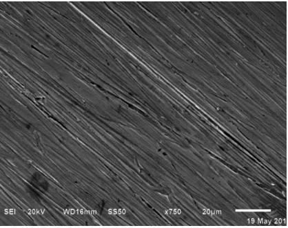
Figures 3(a) and 3(b) represent SEM images of

weld fusion zone before and after pitting corrosion in 1N HCl. The white patches in the SEM image indicate the area subjected to pitting corrosion.

Table 5. Experimental results.

Experiment No.

Pitting corrosion rate

(mm/Year)

Corrosion Rate (mm/Year)

Experimental Predicted

1 0.54120 0.66439

2 0.99950 1.01518

3 0.53390 0.54929

4 0.82320 0.90273

5 0.85370 0.90143

6 0.70170 0.74111

7 0.79770 0.79328

8 0.60120 0.63561

9 0.80370 0.81858

10 0.99020 1.06891

11 0.54110 0.57598

12 0.82740 0.82896

13 1.12450 1.11926

14 0.82460 0.85849

15 0.85000 0.88361

16 0.67440 0.62549

17 0.78280 0.71458

18 0.86260 0.80725

19 1.23460 1.12227

20 0.78540 0.77417

21 0.89920 0.77908

22 0.81610 0.81265

23 0.78220 0.66853

24 0.82250 0.81260

25 0.66290 0.64569

26 0.64746 0.64569

27 0.72800 0.64569

28 0.71500 0.64569

29 0.52060 0.64569

30 0.62900 0.64569

31 0.61690 0.64569

3.1. Developing mathematical model

The output response of the weld joint (Y) is a function of peak current (A), back current (B), pulse rate (C) and pulse width (D). It can be expressed as Eq. (2) [29- 31].

(6)

6

Fig. 3(a). SEM image before corrosion.

Fig. 3(b). SEM image after corrosion.

The second order polynomial equation used to represent the response surface ‘Y’ is given in Eq. (3) [16]:

Y = bo+bi xi +biixi2 + bijxixj+ (3)

where

bi xi indiacte linear terms,

b

ij

x

i

x

j

indicate interaction terms and

biixi

2

represent

pure second order or quadratic effects

. Using MINITAB 14 statistical software package, the significant coefficients were determined and final model was developed using significant coefficients to estimate pitting corrosion rate values of weld joint.

The final mathematical model for pitting corrosion rate is given in Eq. (4).

Pitting corrosion rate (CR) CR= 0.645694+0.023167X1

-0.087025X2+0.008392X3+0.036017X4+0.07563 1X22-0.127775X1X3 (4)

where X1, X2, X3 and X4 are the coded values of peak current, back current, pulse rate and pulse width.

3.2. Checking adequacy of the developed model

Adequacy of the developed model was tested using Analysis of Variance (ANOVA) test. In this technique, if the calculated value of the Fratio of the developed model is less than the standard Fratio (from F-table) value at a desired level of confidence (say 99%), then the model is said to be adequate within the confidence level. ANOVA test results are presented in Table 6 for all the models. According to the table, the developed mathematical models were found to be adequate at 99% confidence level. The value of coefficient of determination ‘ R2 ’ for the above developed models was found to be about 0.86.

Table 6. ANOVA table for pitting corrosion rate.

Pitting corrosion rate

Source DF Seq SS Adj SS Adj MS F P

Regression 14 0.72098 0.72098 0.051499 7.11 0.000

Linear 4 0.22746 0.22746 0.056866 7.85 0.001

Square 4 0.20184 0.20184 0.050461 6.97 0.002

Interaction 6 0.29168 0.29168 0.048613 6.71 0.001

Residual Error 16 0.11590 0.11590 0.007244

Lack-of-Fit 10 0.08727 0.08727 0.008727 1.83 0.237

Pure Error 6 0.02863 0.02863 0.004772

Total 30 0.83689

where DF= Degrees of Freedom, SS=Sum of Squares, MS=Mean Square, F=Fishers ratio.

(7)

7 the actual and predicted values are close to each

other within the specified limits.

3.3. Effect of welding parameters on pitting corrosion rate

3.3.1. Main effects

The above developed mathematical model can be employed to predict the weld pitting corrosion rates and their relationship for the range of parameters used in the investigation by substituting their respective values in the coded form. Based on these models, effects of the process parameters on the weld pitting corrosion rates were computed and plotted, as depicted in Fig. 5.

PREDICTED

A

C

T

U

A

L

1.2 1.1 1.0 0.9 0.8 0.7 0.6 0.5 1.2 1.1 1.0 0.9 0.8 0.7 0.6 0.5

Scatterplot of CORROSION RATE (mm/Year)

Fig. 4. Scatter plot for pitting corrosion rate.

Figure 5 shows that the pitting corrosion rate decreased from 6 Amperes of peak current to

6.5 Amperes and thereafter it increased up to 8 Amperes. Pitting corrosion rates decreased from 3 Amperes of back current to 4.5 Amperes and then increased up to 5 Amperes. Moreover, pitting corrosion rates decreased from 20 pulses/second of pulse rate to 30 pulse/ second and there was increase of up to 60 pulses/second thereafter. They also decreased from 30 % of pulse width to 40% and then increased up to 70 %.

3.3.2. Interaction effects

The simultaneous effect of two parameters at a time on the output response is generally studied using contour plots and surface plots.

3.3.2.1. Contour plots

Contour plots play a very important role in studying the response surface. By generating contour plots using statistical software (MINITAB14) for response surface analysis, the most influencing parameter can be identified based on the orientation of contour lines. If the counter patterning of circular shaped counters occurs, it suggests the equal influence of both factors while elliptical contours indicate interaction of the factors. Figs. 6(a) to 6(c) represent contour plots for pitting corrosion rates. From these plots, the interaction effect between the input process parameters and output response can be observed as:

M

e

a

n

o

f

C

O

R

O

S

IO

N

R

A

T

E

(

m

/

Y

e

a

r)

8 .0 7 .5 7 . 0 6 . 5 6 . 0 1 . 2

1 . 0

0 . 8

5 .0 4 . 5 4 . 0 3 . 5 3 .0

6 0 5 0 4 0 3 0 2 0 1 . 2

1 . 0

0 . 8

7 0 6 0 5 0 4 0 3 0

P EA K C UR R ENT (A m p eres) BA C K C UR R ENT (A m p ere s)

P UL S E R A TE (P u lses/S e co n d ) P UL S E W ID TH (% ) M a i n Effe cts P lot (da ta me a ns ) f or C O R R O S IO N R A TE (mm/ Y e a r )

(8)

8

(i) Pitting corrosion rate was more sensitive to change in peak current than in the base current (Fig. 6(a)) since the contour lines were more diverted towards the peak current.

(ii) Pitting corrosion rate was sensitive to both pulse rate and peak current (Fig. 6(b)) since the contour lines were circular in shape.

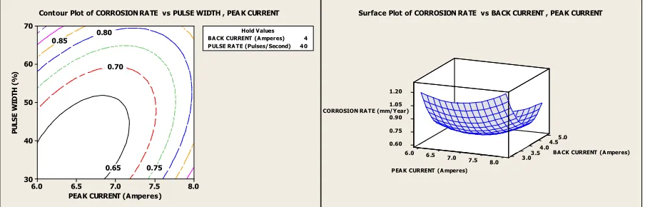
(iii) Pitting corrosion rate was more sensitive to peak current than pulse width (Fig. 6(c)) since the contour lines were more diverted towards the peak current.

From the contour plots, it is clear that the peak current had more effect on corrosion rate.

3.3.2.2. Surface plots

Surface plots help in locating maximum and minimum values of the response. The maximum value of the response is represented by the apex of the surface plot whereas the minimum value is indicated by nadir of the surface plot. Response surface plots clearly indicate the optimal response point. The optimum pitting corrosion rate of pulsed current MPAW welded AISI 304L was exhibited by the nadir of the response surface, as shown in Figs.7(a) to 7(c).

Figure7(a) shows the three dimensional response surface plot for pitting corrosion rate obtained from the regression model, assuming a pulse rate of 40 pulses/second and pulse width

of 50%. The minimum pitting corrosion rate was exhibited by the nadir of the response surface. It can be seen from the twisted plane of surface plot that the model contained an interaction. From the response plot, it could be identified that, at the peak current of 7 Amperes and base current of 4 Amperes, pitting corrosion rate was minimum.

Figure 7(b) depicts the three dimensional response surface plot for the response pitting corrosion rate obtained from the regression model, assuming base current of 4 Amperes and pulse width of 50 %. According to the response plot, it can be identified that, atpeak current of 6 Amperes and pulse rate of 20 pulse/ second, pitting corrosion rate was minimum.

Figure7(c) shows the three dimensional response surface plot for the response pitting corrosion rate obtained from the regression model, assuming base current of 4 Amperes and pulse rate of 40 pulse/second. It can be seen from the twisted plane of surface plot that the model contained an interaction. According to the response plot also, at peak current of 6.5 Amperes and pulse width of 40 %, pitting corrosion rate was minimum.

Based on the surface plots, at peak current of 6 Amperes, Back Current of 4 Amperes, Pulse rate of 40 pulse/second and pulse width of 50%, optimum pitting corrosion rate was obtained.

PEAK CURRENT (Amperes)

B A C K C U R R E N T ( A m p e re s ) 1.1 1.0 0.9 0.8 0.8 0.7 8.0 7.5 7.0 6.5 6.0 5.0 4.5 4.0 3.5 3.0 Hold Values PULSE RA TE (Pulses/Second) 4 0 PULSE WIDTH (%) 5 0

Contour Plot of CORROSION RATE vs BACK CURRENT , PEAK CURRENT

PEAK CURRENT (Amperes)

P U L S E R A T E ( P u ls e s / S e c o n d ) 1.2 1.0 1.0 0.8 0.8 0.6 0.6 8.0 7.5 7.0 6.5 6.0 60 50 40 30 20 Hold Values BA CK CURRENT ( A mperes) 4 PULSE WIDTH (%) 50

Contour Plot of CORROSION RA TE vs PULSE RATE, PEAK CURRENT

(9)

9 PEAK CURRENT (Amperes)

P

U

L

S

E

W

ID

T

H

(

%

)

0.85 0.80

0.75 0.70

0.65

8.0 7.5 7.0 6.5 6.0 70

60

50

40

30

Hold Values BA CK CURRENT (A mperes) 4 PULSE RA TE (Pulses/Second) 4 0

Contour Plot of CORROSION RATE vs PULSE WIDTH , PEA K CURRENT

5 .0 4.5 0.60

0.75

4 .0 0.90

1.05 1.20

BA CK CURRENT (A mperes) 3 .5

6 .0 _{6 .5}

7.0 _7.5 3 .0

8.0 PEA K CURRENT (A mperes)

Surface Plot of CORROSION RATE vs BACK CURRENT , PEAK CURRENT

CORROSION RA TE (mm/Year)

Fig. 6(c). Contour plot for corrosion rate Fig. 7(a). Surface plot for corrosion rate (Peak current vs. Pulse width). (Peak current vs. Back current).

60 5 0 0.50

40 0.75

1.00 1.25 1.50

30 PULSE RA T E (Pulses/Second) 6 .0 _{6 .5}

7.0 7.5 8.0 20 PEA K CURRENT (A mperes)

Surface Plot of CORROSION RATE vs PULSE RATE , PEA K CURRENT

70 6 0 0 .6

0 .7

50 0 .8

0 .9 1 .0

PULSE WIDTH (%) 40

6 .0 _{6 .5}

7.0 7.5 8.0 30 PEA K CURRENT (A mperes)

Surface Plot of CORROSION RA TE vs PULSE WIDTH , PEA K CURRENT

Fig. 7(b). Surface plot for corrosion rate Fig. 7(c). Surface plot for corrosion rate (Peak current vs. Pulse rate). (Peak current vs. pulse width).

4. Conclusions

A five level, four factor full factorial design matrix based on the central composite rotatable design technique was used for the development of mathematical models to predict the pitting corrosion rate of AISI 304L Austenitic stainless sheets welded by pulsed current micro plasma arc welding process. From the contour plots, it was observed that peak current was the most dominating parameter which affected pitting corrosion rate compared to other parameters. According to the surface plots, minimum obtained pitting corrosion rate was 0.64569 mm/Year for the input parameter combination

of peak current of 7Amperes, back current of 4 Amperes, pulse rate of 40 pulses /second and pulse width of 50% whereas the experimental value obtained for the above input parameter combination was 0.52060 mm/Year. It is very clear that the experimental and predicated values were close to each other.

5. Acknowledgements

(10)

10

References

[1] M. Balasubramanian, V. Jayabalan and V. Balasubramanian, “Effect of process parameters of pulsed current tungsten inert gas welding on weld pool geometry of titanium welds”, Acta Metall. Sin.(Engl. Lett.), Vol. 23, No. 4, pp. 312-320, (2010).

[2] B. Balasubramanian, V. Jayabalan and V. Balasubramanian, “Optimizing the Pulsed Current Gas Tungsten Arc Welding Parameters”, J. Mater. Sci. Technol, Vol. 22, No. 6, pp. 821-825, (2006).

[3] K. Siva Prasad , Ch. Srinivasa Rao and D. Nageswara Rao , “Prediction of Weld Pool Geometry in Pulsed Current Micro Plasma Arc Welding of SS304L Stainless Steel Sheets”, International Transaction Journal of Engineering, Management & Applied Sciences & Technologies, Vol. 2, No. 3, pp. 325-336, (2011).

[4] K. S. Prasad, Ch. Srinivasa Rao and D. Nageswara Rao, “A Study on Weld Quality Characteristics of Pulsed Current Micro Plasma Arc Welding of SS304L Sheets”, International Transaction Journal of Engineering, Management & Applied Sciences & Technologies, Vol. 2, No. 4, pp. 437-446, (2011).

[5] K. S. Prasad, Ch. Srinivasa Rao and D. Nageswara Rao, “Optimizing Pulsed Current Micro Plasma Arc Welding Parameters to Maximize Ultimate Tensile Strength of SS304L Sheets Using Hooke and Jeeves Algorithm”, Journal of Manufacturing Science & Production (DyGuter"), Vol. 11, No. 1-3, pp. 39-48, (2011).

[6] K. S. Prasad, Ch. Srinivasa Rao and D. Nageswara Rao, “Effect of Process Parameters of Pulsed Current Micro Plasma Arc Welding on Weld Pool Geometry of AISI 304L Stainless Steel Sheets”, Journal of Materials & Metallurgical Engineering, Vol. 2, No. 1, pp. 37-48, (2012).

[7] K. S. Prasad, Ch. Srinivasa Rao and D. Nageswara Rao, “Establishing Empirical

Relations to Predict Grain Size and Hardness of Pulsed Current Micro Plasma Arc Welded SS 304L Sheets”,

American Transactions on Engineering & Applied Sciences, Vo. 1, No. 1, pp. 57-74, (2012).

[8] K. S. Prasad, Ch. Srinivasa Rao and D. Nageswara Rao, “Effect of pulsed current micro plasma arc welding process parameters on fusion zone grain size and ultimate tensile strength of SSS304L sheets”, International Journal of Lean Thinking, Vo. 3, No. 1, pp. 107-118, (2012).

[9] N. A. Falleiros and S. Wolynec, “Correlation between Corrosion Potential and Pitting Potential for AISI 304L Austenitic Stainless Steel in 3.5% NaCl Aqueous Solution”, Materials Research, Vol. 5, No. 1, pp. 77-84, (2002).

[10] B. Tsaneva, L. Fachikov, Y. Marcheva, M. Lukajcheva and B. Kostadinov, “Corrosion of Chromium Manganese-Nitrogen Steels In Chloride Media”,

Journal of the University of Chemical Technology and Metallurgy, Vol. 42, No. 2, pp. 163-168, (2007).

[11] F. Fauvet, R. Balbaud, Q. Robin, T. Tran, A. Mugnier and D. Espinoux, “Corrosion mechanisms of austenitic stainless steels in nitric media used in reprocessing plants”, Journal of NuclearMaterials, Vol. 375, pp. 52-64, (2008).

[12] D. J. Lee , K. H. Jung , J. H. Sung , Y. H. Kim , K. H. Lee , J. U. Park , Y. T. Shin and H. W. Lee, “Pitting corrosion behavior on crack property in AISI 304L weld metals with varying Cr/Ni equivalent ratio”, Materials and Design, Vol. 30, No. 8, pp. 3269-3273, (2009). [13] A. S. Afolabi, “Effect of Electric Arc

Welding Parameters on Corrosion Behavior of Austenitic Stainless Steel in Chloride Medium”, AU J. T., Vol. 11, No. 3, pp. 171-180, (2009).

(11)

11

Science and Engineering, Vol. 34, No. 2C, pp. 115-127, (2009).

[15] G. Suresh, U. Kamachi Mudali and Baldev Raj, “Corrosion monitoring of type 304L stainless steel in nuclear near-high level waste by electrochemical noise”, J. Appl. Electrochem ,Vol. 41, pp. 973-981, (2011).

[16] Y. Ait Albrimi, A. Eddib, J. Douch, Y. Berghoute, M. Hamdani and R. M. Souto, “Electrochemical Behaviour Of Aisi 316 Austenitic Stainless Steel In Acidic Media Containing Chloride Ions”, Int. J. Electrochem. Sci., Vol. 6, pp. 4614-4627, (2011).

[17] Md. Asaduzzaman, C. M. Mustafa and M. Islam, “Effects of Concentration of Sodium Chloride on the Pitting Corrosion Behavior Of AISI-304L Austenitic Stainless Steel”, Chemical Industry & Chemical Engineering Quarterly, Vol. 17, No. 4 ,pp. 477-483, (2011).

[18] M. Saadawy, Kinetics of Pitting Dissolution of Austenitic Stainless Steel 304 in Sodium Chloride Solution, International Scholarly Research Network, “ISRN Corrosion”, Vol. 2012, Article ID 916367, pp. 1-5, (2012). [19] K. Marimuthu and N. Murugan,

“Prediction and optimization of weld bead geometry of plasma transferred arc hardfaced valve seat rings”, Surf Eng, Vol. 19, No. 2, pp. 143-149, (2003). [20] V. Gunaraj and N. Murugan, “Prediction

and comparison of the area of the heat affected zone for the bead-on-plate and bead-on joint in SAW of pipes”, J. Mat. Proc. Tech., Vol. 95, pp. 246-261, (1999).

[21] V. Gunaraj and N. Murugan, “Application of response surface methodology for predicting weld quality in saw of pipes”, J. Mat. Proc. Tech., Vol. 88, pp. 266-275, (1999).

[22] S. C. Juang, Y. S. Tarng, “Process parameter selection for optimizing the weld pool geometry in the TIG welding of stainless steel”, J. Mat. Proc. Tech., Vol. 122, pp. 33-37, (2002).

[23] T. T. Allen, R. W. Richardson, D. P. Tagliable and G. P. Maul, “Statistical process design for robotic GMA welding of sheet metal”, Weld. J., Vol. 81, No. 5, pp. 69-s-172-s, (2002).

[24] I. S. Kim, J. S. San and Y. J. Jeung, “Control and optimization of bead width for mutipass-welding in robotic arc welding processes”, Aus. Weld. J., Vol. 46, pp. 43-46, (2001).

[25] D. Kim, M. Kang, S. Rhee, “Determination of optimal welding conditions with a controlled random search procedure”, Weld J., pp. 125-s-130-s, (2005).

[26] D. C. Montgomery, “Design and analysis of experiments”, 3rd Edition, NewYork: John Wiley & Sons, pp. 291-295, (1991). [27] G. E. P. Box, W. H. Hunter and J. S.

Hunter, “Statistics for experiments”, New York: John Wiley & Sons, pp. 112-115, (1978).

[28] S. Babu, T. SenthilKumar and V. Balasubram anian, Optimizing pulsed current gas tungsten arc welding parameters of AA6061 aluminium alloy using Hooke and Jeeves algorithm, “Trans .Nonferrous Met. Soc.”China, Vol. 18, pp. 1028-1036, (2008).

[29] W. G. Cochran and G. M. Cox, “Experimental Designs”, London: John Wiley & Sons Inc, (1957).

[30] T. B. Barker, “Quality by experimental design”, Marcel Dekker: ASQC Quality Press, (1985).