Bayesian Combination of Probabilistic Classifiers using
Multivariate Normal Mixtures
Gregor Pirˇs [email protected]
Erik ˇStrumbelj [email protected]
University of Ljubljana
Faculty of Computer and Information Science Veˇcna pot 113, 1000 Ljubljana, Slovenia
Editor:Ryan Adams
Abstract
Ensemble methods are a powerful tool, often outperforming individual prediction models. Existing Bayesian ensembles either do not model the correlations between sources, or they are only capable of combining non-probabilistic predictions. We propose a new model, which overcomes these disadvantages. Transforming the probabilistic predictions with the inverse additive logistic transformation allows us to model the correlations with multivari-ate normal mixtures. We derive an efficient Gibbs sampler for the proposed model and implement a regularization method to make it more robust. We compare our method to related work and the classical linear opinion pool. Empirical evaluation on several toy and real-world data sets, including a case study on air-pollution forecasting, shows that the method outperforms other methods, while being robust and easy to use.
Keywords: correlated classifiers, ensemble, probabilistic models, additive logistic trans-formation, Bayesian inference
1. Introduction
Classifier combination (or ensemble learning) is an important area of applied machine learn-ing and statistics. The idea behind these methods is that combinlearn-ing several prediction mod-els should achieve better performance. Intuitively, if the modmod-els make different mistakes, we can combine them and overcome their individual drawbacks. Zhou (2012) highlights the importance of diversity between individual models and argues that understanding such diversity is an open problem in ensemble learning. A theoretical result on how the gener-alization error of a combination (weighted average of individual methods) decreases as the correlations between individual errors decrease can be found in Ueda and Nakano (1996). That ensembles achieve better performance in practice proved to be the case, as they are extensively used in various machine learning challenges and competitions to great effect— for example an ensemble method won the KDD Cup 2017 (SIGKDD, 2017). The classifiers in an ensemble can be trained on the same data, or on different data sets. In practice, one might want to combine predictions from various sources, for example, a classifier and expert predictions.
Our work was motivated by Kim and Ghahramani (2012) who proposed a Bayesian approach to combining classifiers—the independent Bayesian classifier combination (IBCC)
c
and its dependent extension, the dependent Bayesian classifier combination (DBCC). Their method is able to combine categorical predictions of classifiers, humans, and other sources, not necessarily trained on the same data. They used Markov networks to model the depen-dencies between classifiers. One drawback of their method is that it can only be used to combine non-probabilistic (categorical) classifiers. Another drawback is that the method’s time complexity grows exponentially in the number of classifiers. Simpson et al. (2013) ap-plied the IBCC to a crowdsourcing problem. They observed that the sampler for IBCC can have difficulties with convergence, and proposed a variational IBCC. Additionally Simpson (2014) presented a simplification of Kim and Ghahramani’s IBCC, which led to a more efficient Gibbs sampler for parameter inference. Venanzi et al. (2014) extended the IBCC specifically for crowdsourcing problems. They proposed CommunityBCC, where each source (worker) is assumed to belong to some community with a common confusion matrix. The method is able to model the dependencies implicitly through community membership. The results show that CommunityBCC outperforms IBCC on sparse data sets. Naz´abal et al. (2016) extended the IBCC model to combine probabilistic models by modeling the predic-tions with the Dirichlet distribution, however they do not model correlapredic-tions explicitly.
Another approach that is closely related to IBCC are supra-Bayesian methods, which rely on Bayes’ rule to combine the information gathered from several experts and thus improve the predictions. They assume a multivariate normal (MVN) distribution of the predictions and are therefore able to model correlations. Lindley (1985) presented a method for combining probabilistic predictions of categorical data. The author proposed modeling of log-odds instead of original data to deal with the non-normality. The method also uses a common covariance matrix, independent of true labels. Due to the use of a MVN distribution and the assumption of a common covariance matrix the described method lacks flexibility to model the latent space well.
Hoeting et al. (1999) presented Bayesian model averaging that combines several prob-abilistic models, weighted by their posterior probability. However this approach assumes that one of the combining models is the true data generating model and that the mod-els represent mutually exclusive situations. These assumptions can lead to severe loss of performance, as Cerquides and De M´antaras (2005) have shown.
Lacoste et al. (2014) proposed the agnostic Bayesian learning of ensembles, where they produced ensembles of predictors based on holdout estimations of their generalization per-formances. Their ideas are based on the inductive learning paradigm and they use Bayesian treatment to find the posterior probability of each hypothesis being the best. They defined the risk of each hypothesis as its expected loss and examined various priors over the joint risk. The inputs to the model can be probabilistic and they account for correlations between inputs. Agnostic Bayes differs from IBCC, its extensions, and supra-Bayesian methods, as it focuses on finding the best performing models and weighting them accordingly, as opposed to relying on finding a latent structure of the predictions.
the model with a fully Bayesian framework and use Gibbs sampling (Casella and George, 1992) for parameter inference. Since the complexity of the model grows with the number of classifiers, we implement a regularization method, which makes the model more robust. Our method can also be viewed as an extension of the supra-Bayesian method, where we use mixtures of normals as the likelihood and condition the means and covariance matrices on the true label—increasing the method’s flexibility.
We empirically evaluated our method on several toy and real-world data sets, and com-pared it to related methods. The results on toy data sets highlight that none of the en-sembles works well for all data sets. Overall, our method compares favourably to related methods. Additionally, we provide a case study on combining predictions of air-pollutant concentration in Slovenia, where we show that our method is well suited for combining machine learning models with human expert predictions.
The paper is organized as follows. In Section 2 we formulate the problem, present our main methodological contribution, and provide a description of related work. We present the data sets, empirical results, and a case study in Section 3. We discuss the results and provide directions for future work in Section 4.
2. Methods
Let {ti}ni=1 be our data set of n observations that can take one of m different values ti ∈ {1, . . . , m}. Additionally, we have r sources of probabilistic predictions and, for
each source, a probabilistic prediction for each observation {p(1)i , . . . , p(r)i }n
i=1, wherep (k) i = h
p(k)i1 · · · p(k)im iT
is the k−th source’s prediction for thei−th observation.
The task is to learn how to combine individual sources into more accurate probabilistic predictions, so that we are able to produce probabilistic predictions{pˆi}n+n
∗
i=1 fornobserved
and n∗ future/unobserved data, represented with categorical random variables {Ti}n+n ∗ i=n+1,
for which only the sources’ predictions {p(1)i , . . . , p(r)i }n+ni=n+1∗ are known.
2.1. MVN Mixture Conditional Likelihood Model (MM)
Aitchison (1982) proposed the modeling of correlated data on a simplex with the logit-normal distribution. The data on a simplex are considered as data drawn from a MVN dis-tribution, transformed by the additive logistic transformation. This transformation trans-forms a vectorx∈Rzinto a vectorf(x)∈Sz+1, whereSz+1represents a (z+1)-dimensional
simplex. To model the correlations between probabilistic predictions we first transform each source’s prediction with the inverse of the additive logistic transformation. Applying it to
{p(1)i , . . . , p(r)i }i=1n+n∗, we get {u(1)i , . . . , u(r)i }n+ni=1∗, where u(k)i = hu(k)i1 · · · u(k)i(m−1)iT. Let
ui = h
u(1)Ti · · · u(r)Ti i
, be the concatenated vector of u(k)i s, where k = 1, ..., r. The di-mension of ui is then r(m−1), the number of sources times the number of classes minus
one. Then the vectors ui, can be modeled by a MVN distribution, as described above.
However, the transformation does not guarantee a MVN distribution of ui and in practice
Our generative model can be described as follows. The probabilistic predictions p(k)i =
h
p(k)i1 · · · p(k)im iT
are generated by applying the additive logistic transformation to realiza-tions of MVN mixtures, whose parameters depend on the true label. The probability for a new observation to be in true labelj is then proportional to the density of the correspond-ing MVN mixture. The true labels {ti}ni=1 and {Ti}n+n
∗
i=n+1 are assumed to be generated
by a categorical distribution with parameter ρ, and we set a Dirichlet prior on ρ, same as Naz´abal et al. (2016). The mixture memberships gi are assumed to be generated by a
categorical distribution of dimension d. For the parameters of MVN distributions we set semi-conjugate MVN and inverse-Wishart priors. We write the likelihood and the priors as
ui|ti =j, gi =h, µ,Σ∼ Nr(m−1)(µjh,Σjh), (1)
ti|ρ∼Cat(ρ), (2)
ρ|γ0∼Dir(γ0), (3)
gi∼Cat(τ0), (4)
µjh∼ Nr(m−1)(µ0,Σ0), (5)
Σjh∼inv-Wishart(ν0, S0−1), (6)
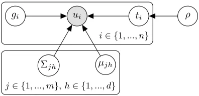
whereµ={µjh:j= 1, ..., m∧h= 1, ..., d}, Σ ={Σjh :j= 1, ..., m∧h= 1, ..., d}. Figure 1
shows the proposed model in plate notation. Let vectors ui = h
u(1)Ti · · · u(r)Ti i
form the rows of matrix U. Our goal is to sample from
Z
p(T, ρ, g, µ,Σ|U, t)dρ=p(T, g, µ,Σ|U, t). (7)
To simplify the sampling we marginalize over ρ. Therefore, we need to sample T, µ, Σ, and g. In the remainder of the section we derive full-conditional distributions for these variables and construct a Gibbs sampler. We infer the parametersµ, Σ, and g only on the data where the true label is known, however, the method would also allow inference over unlabelled data.
First we observe that full-conditional distributions of µ and Σ are conditionally inde-pendent of ρ and proportional to the product of likelihood and the respective prior. Let
ui ti
gi
i∈ {1, ..., n}
Σjh µjh
j∈ {1, ..., m},h∈ {1, ..., d}
ρ
Figure 1: Bayesian plate notation for the proposed model. The transformed predictions
ui for thei−th observation are assumed to be generated conditional on the true
label ti =j from the corresponding MVN distribution with parameters µjh and
Σjh, which also depend on the latent group gi =h. The true label is distributed
categorically with parameterρ. Priors are omitted for brevity.
µjh|U, t, ρ, g,Σ∼ Nr(m−1)(µ∗,Σ∗), (8)
Σjh|U, t, ρ, g, µ∼inv-Wishart(ν∗, S∗−1), (9)
µ∗ = Σ∗(Σ−10 µ0+njhΣ−1jhu¯(jh)),
Σ∗ = (Σ−10 +njhΣ−1jh)−1, ν∗ =ν0+njh,
S∗ =S0+ njh
X
l=1
(u(jh)l −µjh)(u(jh)l −µjh)T,
wherenjh is the number of true labels equal toj in grouph and ¯u(jh)are the column means
of U(jh).
The mixture membership variable g is also conditionally independent of ρ. Using Eq. (1) and (4), the full-conditional ofg is
p(g|U, t, ρ, µ,Σ)∝p(U|g, t, ρ, µ,Σ)p(g, t, ρ, µ,Σ)
∝ n Y
i=1
p(ui|gi, ti, ρ, µ,Σ)
p(g)
∝ n Y
i=1
p(ui|gi, ti, µ,Σ)p(gi). (10)
For the predictive distribution of a new observation Ti, we do not have samples of gi.
Therefore we need to marginalize over gi. Using Eq. (1), (2), and (3), the full-conditional
p(Ti =j|U, t, ρ, g, µ,Σ)∝ Z d
X
l=1
p(Ti =j, gi=l, U, t, ρ, g, µ,Σ)dρ
∝ Z d
X
l=1
p(ui|Ti =j, gi=l, t, ρ, g, µ,Σ)p(Ti =j, gi=l, t, ρ, g, µ,Σ)dρ
∝ Z d
X
l=1
p(ui|µjl,Σjl)p(gi =l|Ti =j, g)p(Ti =j, t, ρ)dρ
∝ d X
l=1
p(ui|µjl,Σjl)p(gi =l|Ti =j, g) Z
p(Ti =j, ρ)p(t|ρ)p(ρ)dρ,
(11)
where we integrate over all ρ ∈Sm. The integral in Eq. (11) can be solved by observing that the expression is the multivariate beta function. Some algebra with gamma functions leads to (γ0j +nj), where nj =Pnl=1I(tl=j). Additionally let ngjl =p(gi =l|Ti=j, g) =
|{gs=l∧ts =j :s= 1, . . . , n}|/|{ts =j :s= 1, . . . , n}|, which represents the probability
of the new observation being in a specific mixture. Inserting this into Eq. (11) and using Eq. (8), (9), and (10) we construct a Gibbs sampler for Eq. (7)
µjh|U, t, ρ, g,Σ∼ Nr(m−1)(µ∗,Σ∗),
Σjh|U, t, ρ, g, µ∼inv-Wishart(ν∗, S∗−1),
p(gi =h|U, ti =j, ρ, µ,Σ)∝p(ui|µjh,Σjh)τ0h, p(Ti=j|U, t, ρ, g, µ,Σ)∝
d X
l=1
ngjlp(ui|µjl,Σjl)(γ0j+nj),
where we use the conditional independence of group memberships in Eq. (10) and sample each gi separately. Due to an efficient group collapsing property, the number of mixture
groupsdcan be set to some arbitrary high number and the model finds the suitable number automatically. Some groups tend to be closer together at the beginning. This causes the data points to interchange between groups and pairs of groups often merge into one, resulting in fewer mixture components.
If we constrain the covariance matrices Σ to be diagonal, the model is still able to find mixture-components where the correlations are relatively low. This way the correlations are still modelled, while the method becomes less complex. Therefore, we can exchange some flexibility for simplicity, which results in faster inference (inverse of the covariance matrices becomes trivial), while still remaining flexible enough to model the correlations well in most situations. We included this method in the empirical evaluation (MM-diag).
2.1.1. Regularization
λ∗i ≥0. We modify Eq. (11) by changing p(ui|µjl,Σjl) to p(ui|µjl,Σjl+ diag(λ∗)). Adding
a positive number to an element on the diagonal increases the variance of the density, reducing the variance of the data in that dimension (and their covariance with all other dimensions). This effectively decreases the differences in density (between observations) in that dimension. That is, it reduces the influence of that dimension on the distribution of
Ti.
For each Gibbs iteration, the λ∗ for that iteration is determined before predicting for the unobserved dataT using
p(λ|U, t, ρ, g, µ,Σ)∝p(ti =ji|U, t, ρ, g, µ,Σ, λ)p(λ),
whereji is the true class label for examplei.
In general, we could make our predictions by integrating overλ. However, the posterior dis-tribution forλis intractable and in practice typically very difficult to sample from efficiently. For the purposes of this work, we use only the MAP estimate
λ∗= arg max
λ
logp(λ) +
n X
i=1
logp(ti=ji|U, t, ρ, g, µ,Σ, λ).
2.2. Related Work
To empirically evaluate our method, we also implemented four Bayesian approaches to combining classifiers and the classical linear opinion pool.
2.2.1. Supra-Bayesian
Lindley (1985) presented the supra-Bayesian method for combining probabilistic predictions of a categorical variable of r experts. The method relies on Bayes’ theorem to calculate the posterior distribution of predictions of the decision maker, given the predictions of the experts. Let A1, A2, ..., Am be the possible outcomes of the categorical variable and let S1, S2, ..., Sr be classifiers. LetH be the decision maker’s prior probability for the response
and qij = log(Pri(Aj)) the log-probability assigned to true label Aj by the i−th classifier.
Then the decision maker updates his probabilities via the Bayes’ theorem
p(Aj|Q, H)∝p(Q|Aj, H)p(Aj|H). (12)
To model the correlations between given predictions, Lindley proposes a MVN dis-tribution for p(Q|A, H). Additionally, Lindley argues that the classifiers’ belief in their prediction is independent of the label of their prediction, therefore the MVN distributions share a common covariance matrix between predictions for different labels. The author also proposes the modeling of log-odds instead of log-probabilities, as log-odds are expected to be distributed normally. We implemented a ML estimation of the multivariate parameters for Eq. (12), where the matrixQ represented log-odds.
2.2.2. IBCC
IBCC (Kim and Ghahramani, 2012) assumes that the true labels t are generated by a categorical distribution with parameter κ. The prediction c(k)i of individual classifier k is also generated by a categorical distribution with parameters πj(k) for each possible value j
of the true label. Let ν be the prior for κ and α(k)0,j prior for πj(k). Kim and Ghahramani additionally put an exponential prior onα(k)0,j, but Simpson (2014) observed that the model without this additional flexibility performs comparably well and derived the Gibbs sampler forκ, Π, and the true labels
p(κ|t, ν0) =
1
B(ν)
m Y
j=1 κνj
j ,
p(πj(k)|t, c, α(k)0,j) = 1
B(α(k)ti )
m Y
l=1
π(k)j,l α (k)
j,l ,
p(ti =j|Π, κ, c)∝κj r Y
k=1 π(k)
j,c(ik),
whereνj =ν0,j+Pn+n ∗
i=1 δ(ti−j) andα(k)j,l =α(k)0,j,l+Pn+n ∗
i=1 δ(ti−j)δ(c(k)i −l).
2.2.3. IBCC QPI
The IBCC method can be extended to allow for quasi-probabilistic inputs (QPI).
Proba-bilistic classifiers provide us with probabilities of each outcome p(k)i =
h
p(k)i1 · · · p(k)im iT
. For the IBCC to exploit probabilistic predictions, we can first take a sample from a categor-ical distribution with parameter p(k)i for each source k. The categorical samples can then be represented as binary vectors, which are of appropriate form for the inputs of IBCC. We then takentsamp such samples and use them to create a new training set of sizen×ntsamp.
For prediction, we use the same procedure. We sample according to the sources’ proba-bilistic predictions. We retrieve the final prediction as the average probaproba-bilistic prediction over all samples. This allows the IBCC to take advantage of probabilistic predictions, instead of simply using the class with the highest probability, as the sources’ predictions.
2.2.4. Agnostic Bayes
The agnostic Bayes approach (Lacoste et al., 2014) combines sources based on the probabil-ity of being thebest source, where best is defined in terms of some task-dependent measure. The combined prediction is defined as
ˆ
pi = r X
k=1
P(k?=k|p, t)p(k)i ,
log-score performance measure, we can simplify P(k? = k|p, t) = P(∀k0 ∈ 1..r :E[l(k)]≥ E[l(k0)]|l) = P(k|l), where E[l(k)] is the k−th source’s expected log-score and l all the observed log-scores (for this model, a sufficient statistic forp and t).
We draw samples from P(k|l) with bootstrap inference (this was shown to be very effective in Lacoste et al. 2014, at least as effective as placing priors over joint risk and performing Bayesian inference). That is, we draw a replacement set of observations and compute the average log-score. This gives us the best source on this replacement set—one sample fromP(k|l). The process is repeated for several iterations to obtain a set of samples that approximateP(k|l).
2.2.5. Linear Opinion Pool (LOP)
The linear opinion pool (Cooke et al., 1991) is the classical approach to combining pre-dictions. The combined prediction ˆpi is expressed as a linear combination of individual
sources
ˆ
pi =Xiβ,
whereXi=
p(r)i p (r−1)
i · · · p (1) i p
(0) ·
and β =
βr βr−1 · · · β1 β0 T
.
The parametersβi andp(0)· were fit by maximizing the likelihood, subject to 0≤βi ≤1, Pr
i=0βi= 1, 0≤p(0)ij ≤1, and Pm
j=1p (0)
·j = 1.
We also included a combination of LOP and MM, where the probabilistic predictions obtained by MM are added to the sources before LOP is applied (LOP+MM).
2.2.6. Discussion of Related Work
We can divide the methods for classifier combination into two groups. Methods that aim to estimate the performance of each classifier and then weigh their predictions by their per-formance (LOP, agnostic-Bayes, etc.). And methods that aim to learn the latent structure of the classifications and then provide probabilistic classifications (IBCC and extensions, supra-Bayesian, etc.).
The former are expected to perform poorly when there is a latent structure to learn, for example, biased classifiers or systematic errors in classifiers. On the other hand, these methods have an advantage that they are not expected to perform discernibly worse than the best source. The latter are the exact opposite—they can learn complex latent structure and perform better than the first group, but can also perform extremely poorly, discernibly worse than the best source. In Section 3 we present 5 toy data sets, which serve to show the differences in performance of these groups, depending on the structure of the data.
IBCC QPI is similar to MM in that it is able to exploit probabilistic nature of predictions, however it does not model correlations.
Naz´abal et al. (2016) used a Dirichlet distribution to model probabilistic outputs of the sources. A similar (but not equivalent) model would result if we used diagonal covariances without mixtures in the proposed MM. Therefore the proposed MM improves on the draw-backs of Naz´abal et al. as it allows for the modeling of correlations between sources, and additionally adds flexibility through the use of mixtures.
MM could also be interpreted as a regularized supra-Bayesian method with MVN-mixture likelihood. The modeling of log-odds described by Lindley (1985) is equivalent to the modeling of the transformed classifiers by MM. A major difference between the methods is that MM does not assume the same covariances over all true labels. Further-more, each mixture component has its own covariance matrix, which further improves the flexibility of our method.
3. Empirical Evaluation
We empirically evaluated and compared the methods on several toy and real-world data sets. We estimated out-of-sample log-score using train-test splits. To compare the best-performing method with the rest, we used the differences between log-scores. Let abe the vector of lengthntof log-scores of the best performing method,bthe vector of log-scores of
another method, and d=a−b. If
1
nt nt
X
i=1 di
>2
s
VAR[d]
nt ,
we argue that there is a discernible difference in performance. Details on how the data were generated and split are provided below.
For IBCC and its extension, we selected priors that assume each class has the same prior probability. We used the same priors (α0,j = 1) for all confusion matrices, which represents
a weak belief that the models are random. For MM we selected vague priors that put prior belief that the mean values of transformed predictions are zero with large variances. However, MM has proved to be somewhat robust to the prior selection. We set the same priors for Bayesian methods over all data sets. Forλ, we use uniform priorsλi∼iid U(0,105).
We set the maximum number of mixture components for MM to 15, however this number dynamically falls, depending on the problem, as we described in Section 2.1.
3.1. Data Sets
In this section we describe the data sets we used for empirical evaluation.
3.1.1. Toy Data Sets
The data set has a target variable with three possible outcomes. The target vari-able’s value is generated for each sample i separately by first drawing the underlying probability vector p∗i from Dirichlet(1.5,0.9,0.6) and then drawing the target value from Categorical(p∗i). We generated 500 samples for training and 5000 samples for testing.
We then generated the following sources of probabilities, based on the underlying prob-ability vectorsp∗:
• Random 1 & 2: The probabilities are drawn independently for each sample from Dirichlet(1,1,1).
• Good 1 & 2: The probabilities are drawn independently for each sample from Dirichlet(10p∗i).
• Permuted 1: The probabilities are drawn independently for each sample from
Dirichlet(100p∗i) and permuted (2, 3, 1). This results in a source that gives very accurate probabilities, but does not correctly assign them to the possible values of the target variable.
• Permuted 2: Identical to Good 2, but permuted (2, 3, 1).
The two sources, Source 1 and Source 2, were assigned as follows: toy A (Random 1, Random 2), toy B (Good 1, Random 1), toy C (Good 1, Good 2), toy D (Good 1, Permuted 1), andtoy E(Good 1, Permuted 2).
3.1.2. Bookies
Each sample in this data set is a football game and the four sources of probabilistic predic-tions are four major online bookmakers. Probabilistic predicpredic-tions were calculated by nor-malizing the reciprocals of odds offered for the outcome of the game (home, draw, away). Therefore, the target variable has 3 outcomes. The data set has 5434 samples, we used 2000 for training and 3434 for testing. Bookmakers are very good sources of probabilistic predictions (Forrest et al., 2005) and their predictions are highly correlated—the lowest correlation is 0.92. We do not expect any ensemble method to outperform the best source.
3.1.3. DNA
Two data sets were constructed using the StatLog DNA data set in a way similar to the experiments in Kim and Ghahramani (2012).
DNA A:2000 samples were partitioned into 5 partitions, 400 samples each, and a C4.5 decision tree classifier was trained on each partition. These classifiers were used to classify the remaining 1186 samples, 400 of which were used for training and 786 for testing.
3.2. Results
The results are shown in Table 1. No method clearly outperforms other methods over all data sets. LOP and MM perform well on most data sets. For LOP the exceptions are data sets with a more complex relationship between the sources’ predictions and the outcome (toy D). And for MM the exceptions are the two simple toy data sets with a continuous relationship between the sources’ predictions and the probability of the outcome (toy B, toy C). MM-diag performs worse than the MM on all data sets, however, the differences are small on average. A combination of LOP and MM nullifies the drawbacks of each individual method and performs the best on average. Toy D, with systematic errors in otherwise good sources, is a good example of a data set where the methods that rely on finding the best source are inferior to models that learn the latent structure, providing a good argument for the latter.
Agnostic Bayes will assign a lot of weight to the best source, unless it is difficult to discern the best source. The latter is in cases where there is not a lot of data, relative to the magnitude of the differences between the sources in terms of performance (toy A, DNA A). Therefore, as expected, it performs well when the most accurate source performs well (toy B, toy C, toy E, bookies), and performs poorly, when it does not (DNA B). Note that there is no correlation between the true labels and sources in the toy A data set—the best possible model would assign the same probabilities to all outcomes. Agnostic Bayes performs poorly because it tries to identify the best performing model, but none of the sources perform well. The same would happen to LOP if we did not include an intercept term.
IBCC performs poorly on the toy data sets but performs well on the DNA data sets. However, it is strictly outperformed by MM. The quasi-probabilistic IBCC outperforms the IBCC on DNA data sets and performs similarly on most of the toy data sets. Furthermore, it performs well on the toy A data set, where it is the best performing model, with the proposed MM showing a similar level of performance. IBCC QPI therefore proved to be better suited for probabilistic input than the IBCC, as expected. The supra-Bayesian approach of Lindley (1985), which can be viewed as a very simple case of the proposed approach, performs the worst on average, among all the Bayesian approaches.
Ba
yesian
Combina
tion
of
Pr
obabilistic
Classifiers
MM Source 1 LOP+MM MM-diag agnostic agnostic MM MM
−−−1.031±0.005 −−−0.831±0.009 −−−0.811±0.008 −−−0.002±0 −−−0.826±0.009 −−−0.966±0.008 −−−0.206±0.025 −−−0.132±0.028
MM-diag LOP agnostic LOP+MM Source 1 LOP+MM LOP IBCC QPI
−−−1.032±0.006 −−−0.831±0.009 −−−0.822±0.009 −−−0.007±0 −−−0.826±0.009 −−−0.967±0.008 −−−0.22±0.026 −−−0.134±0.023
LOP LOP+MM Source 1 IBCC MM LOP agnostic MM-diag
−−−1.032±0.005 −−−0.831±0.009 −−−0.826±0.009 −−−0.018±0 −−−0.83±0.007 −−−0.967±0.007 −−−0.22±0.02 −−−0.139±0.027
LOP+MM Supra MM Supra LOP Source 3 MM-diag LOP
−−−1.032±0.006 −−−0.892±0.008 −−−0.828±0.007 −−−0.111±0.001 −−−0.83±0.008 −−−0.968±0.007 −−−0.222±0.03 −−−0.157±0.016
IBCC MM Source 2 IBCC QPI MM-diag MM IBCC QPI IBCC
−−−1.043±0.006 −−−0.893±0.006 −−−0.832±0.009 −−−0.204±0.001 −−−0.838±0.007 −−−0.968±0.008 −−−0.248±0.033 −−−0.181±0.033
Supra MM-diag MM-diag agnostic Supra Source 4 IBCC agnostic
−−−1.107±0.002 −−−0.906±0.006 −−−0.839±0.008 −−−0.824±0.009 −−−0.883±0.007 −−−0.968±0.007 −−−0.271±0.037 −−−0.182±0.033 agnostic IBCC Supra Source 1 IBCC QPI Source 2 Supra Source 2 −−−1.259±0.009 −−−0.921±0.008 −−−0.883±0.007 −−−0.824±0.009 −−−0.908±0.005 −−−0.969±0.007 −−−0.275±0.017 −−−0.182±0.033
Source 2 IBCC QPI IBCC QPI LOP IBCC MM-diag Source 4 Supra
−−−1.469±0.015 −−−0.953±0.005 −−−0.907±0.005 −−−0.835±0.008 −−−0.92±0.012 −−−0.969±0.008 −−−0.461±0.055 −−−0.214±0.013 Source 1 Source 2 IBCC Source 2 Source 2 IBCC QPI Source 5 Source 4 −−−1.508±0.016 −−−1.469±0.015 −−−0.919±0.012 −−−3.081±0.006 −−−1.43±0.011 −−−0.993±0.006 −−−0.767±0.074 −−−0.311±0.011
Supra Source 3 Source 3 −
−−1.008±0.007 −−−0.784±0.075 −−−0.321±0.046 IBCC Source 2 Source 5 −
−
−1.245±0.02 −−−0.846±0.078 −−−0.587±0.01 Source 1 Source 1 −
−−0.879±0.079 −−−4.305±0.717
Table 1: Estimated log-scores and standard errors on toy and real-world data sets. For each data set, the methods are ordered in descending order of performance. Highlighted methods are not discernibly worse than the best-performing method for that data set.
3.3. Case Study—Prediction of Air-Pollutant Concentration
Air pollution poses a great risk for public health (World Health Organization, 2014). Fore-casting excessive air pollution is an important task, also regulated by a EU directive (Eu-ropean Council, 2008). In Slovenia, the Slovenian Environment Agency (ARSO) is tasked with forecasting daily average concentration of particulate matter (PM10) and daily
maxi-mum concentration of tropospheric ozone (O3) for the same day (in the morning) and the
next day. Currently, models and human experts are used for this task. Faganeli Pucer et al. (2018) proposed a Bayesian methodology for this problem and empirically compared several machine learning methods and human experts. Gaussian processes performed the best on average, but the question remains whether an ensemble method can be used to improve on individual models. With that aim, we evaluate methods from Section 2 on four air-pollution data sets used in Faganeli Pucer et al. (2018).
The data sets consist of measurements of daily levels of PM10 and O3 on several
sta-tions across Slovenia from 2013 to 2016. The data were provided by ARSO. According to reporting guidelines, PM10 levels are categorized into three categories: 0-35 µg/m3, 35-50
µg/m3, greater than 50 µg/m3, and O3 levels are categorized into four categories: 0-60
µg/m3, 60-120 µg/m3, 120-180µg/m3, greater than 180 µg/m3.
Three prediction models—Bayesian lasso, random forests, and Gaussian processes—and human expert predictions were used to predict the levels for the same and next day, depend-ing on covariates available at the current day. Expert predictions were non-probabilistic (categorical). The models were trained in a time-respecting manner (predictions for 2014 were obtained by training the models on data from 2013, predictions for 2015 were ob-tained by training the models on data from 2013 and 2014, etc.). We used two thirds of observations for training and the rest for testing.
The empirical results for the case study are shown in Table 2. The combination of MM and LOP performs the best over all data sets. MM and LOP are the only methods that show no discernible differences to LOP+MM over all data sets. This provides a strong argument for our method, compared to other methods which learn the latent structure of the data. MM also strictly outperforms MM-diag, as expected. IBCC QPI performs well on the PM10 data sets, however it does not outperform MM. Agnostic Bayes performs slightly
better than the best source on all data sets, however it is discernibly worse than the best method on two data sets. The other methods are unable to outperform the best performing individual classifier on all data sets.
The major arguments for our method are twofold. First, it is a step forward in the state-of-the-art methods which rely on learning the latent structure of the data (IBCC, IBCC QPI, Supra). This can be seen as it is the only such method which is never discernibly worse than the best performing method. Second, LOP+MM performs the best on all data sets in the case study. It also outperforms LOP on all real-world data sets, which is discernibly better—it is highly unlikely that this is due to chance.
4. Conclusion
PM10 tomorrow PM10 today O3 today O3 tomorrow
LOP+MM LOP+MM LOP+MM LOP+MM
− −
−0.613±0.022 −−−0.406±0.019 −−−0.375±0.025 −−−0.439±0.027
MM MM LOP LOP
− −
−0.613±0.023 −−−0.409±0.021 −−−0.378±0.024 −−−0.442±0.028
MM-diag LOP MM MM
− −
−0.62±0.023 −−−0.419±0.019 −−−0.389±0.028 −−−0.446±0.029
IBCC QPI MM-diag agnostic agnostic
− −
−0.62±0.024 −−−0.419±0.021 −−−0.393±0.027 −−−0.463±0.028
LOP IBCC QPI Source 1 Source 1
− −
−0.634±0.02 −−−0.436±0.024 −−−0.393±0.027 −−−0.463±0.028
agnostic agnostic MM-diag MM-diag
− −
−0.684±0.026 −−−0.442±0.023 −−−0.393±0.027 −−−0.471±0.034
Source 2 Source 1 IBCC QPI IBCC QPI
− −
−0.684±0.026 −−−0.442±0.023 −−−0.394±0.028 −−−0.49±0.032 Source 1 Source 2 Source 2 Source 2 −
−
−0.703±0.019 −−−0.516±0.015 −−−0.462±0.02 −−−0.508±0.021
Supra Supra Source 3 Source 3
− −
−0.732±0.017 −−−0.533±0.018 −−−0.511±0.033 −−−0.53±0.022
IBCC Source 3 IBCC Supra
− −
−0.791±0.038 −−−0.641±0.041 −−−0.563±0.053 −−−0.808±0.031
Source 3 IBCC Supra IBCC
− −
−0.896±0.042 −−−0.673±0.041 −−−0.683±0.036 −−−0.83±0.067 Source 4 Source 4 Source 4 Source 4 −−−2.23±0.09 −−−1.578±0.081 −−−1.18±0.101 −−−1.371±0.108
correlations between the classifiers. We derived an efficient Gibbs sampler for our method, along with a regularization method for robustness.
The results on toy data sets highlighted that there is no single method that performs well over several diverse data sets. However, our method outperforms related Bayesian methods on all but one real-world data sets. The method proved to be especially useful in the case study, where we combined three machine learning methods and human expert predictions for air-pollutant concentration forecasting. This case study illustrates the main use-case for our method—a relatively small number of probabilistic or crisp (0/1) sources, which are potentially flawed (biased, etc.) and correlated. Our method is also very robust and requires practically no tuning. Additionally, a combination of linear opinion pool and our method proved to be very successful, outperforming all methods on all but one real-world data sets, and also being robust on the difficult toy data sets.
Our method still has some drawbacks, however. The original model is based on full covariance matrices, so the number of the parameters grows quadratically with the number of possible outcomes and the number of classifiers. While this is an improvement over the exponential growth in the number of classifiers of the DBCC model, it still leads to very complex models in high dimensions. One possibility of at least partially regulating this drawback is to constrain the covariance matrices to being diagonal—as in our empirical evaluation. Alternatively, we could assume the same covariance matrix over all mixture components in a true label, or assume the same variances/covariances over several predic-tions. We leave the analysis of possible constraints for future work. As part of future work, we will also explore if the predictive performance or robustness of the method could be im-proved by using Gaussian processes and/or variational autoencoders instead of multivariate normal mixtures to model the sources’ transformed probabilities. Additionally, we could limit the computational complexity by using sparse Gaussian processes.
As is the case in other areas of learning, there is no single best method of combining probabilistic predictions. In some cases, the best approach is to combine the sources based on their predictive performance or to directly maximize the predictive performance of the combination, such as agnostic Bayes or the linear opinion pool. However, sometimes there are more complex relationships between classifiers and the target variable and methods that are able to learn these patterns will perform better. In such cases, our method is in several ways a superior alternative to existing Bayesian approaches. It is able to model complex relationships, while still being robust and easy to tune, thus providing us with a useful approach for combining probabilistic predictions.
Acknowledgments
References
John Aitchison. The statistical analysis of compositional data. Journal of the Royal Statis-tical Society. Series B (Methodological), pages 139–177, 1982.
George Casella and Edward I. George. Explaining the Gibbs sampler. The American Statistician, 46(3):167–174, 1992.
Jes´us Cerquides and Ramon L´opez De M´antaras. Robust Bayesian linear classifier ensem-bles. In European Conference on Machine Learning, pages 72–83. Springer, 2005.
Roger Cooke et al. Experts in uncertainty: opinion and subjective probability in science. Oxford University Press on Demand, 1991.
European Council. Directive 2008/56/EC of the European Parliament and of the Council.
Decision of Council, 2008.
Jana Faganeli Pucer, Gregor Pirˇs, and Erik ˇStrumbelj. A Bayesian approach to forecasting daily air-pollutant levels. Knowledge and Information Systems, pages 1–20, 2018.
David Forrest, John Goddard, and Robert Simmons. Odds-setters as forecasters: The case of English football. International Journal of Forecasting, 21(3):551–564, 2005.
Jennifer A. Hoeting, David Madigan, Adrian E. Raftery, and Chris T. Volinsky. Bayesian model averaging: a tutorial. Statistical Science, pages 382–401, 1999.
Hyun-Chul Kim and Zoubin Ghahramani. Bayesian Classifier Combination. InInternational Conference on Artificial Intelligence and Statistics, pages 619–627, 2012.
Alexandre Lacoste, Mario Marchand, Fran¸cois Laviolette, and Hugo Larochelle. Agnostic Bayesian learning of ensembles. InInternational Conference on Machine Learning, pages 611–619, 2014.
Dennis V. Lindley. Bayesian Statistics 2, chapter Reconciliation of discrete probability distributions, pages 375–391. North-Holland, 1985.
Alfredo Naz´abal, Pablo Garc´ıa-Moreno, Antonio Art´es-Rodr´ıguez, and Zoubin Ghahramani. Human activity recognition by combining a small number of classifiers. IEEE Journal of Biomedical and Health Informatics, 20(5):1342–1351, 2016.
SIGKDD. KDD Cup 2017: Highway tollgates traffic flow prediction. http://www.kdd.org/ kdd2017/News/view/announcing-kdd-cup-2017-highway-tollgates-traffic-flow-prediction, 2017. Accessed: 2018-04-05.
Edwin Simpson. Combined decision making with multiple agents. PhD thesis, University of Oxford, 2014.
Naonori Ueda and Ryohei Nakano. Generalization error of ensemble estimators. In IEEE International Conference on Neural Networks, pages 90–95. IEEE, 1996.
Matteo Venanzi, John Guiver, Gabriella Kazai, Pushmeet Kohli, and Milad Shokouhi. Community-based Bayesian aggregation models for crowdsourcing. InInternational Con-ference on World Wide Web, pages 155–164. ACM, 2014.
World Health Organization. Ambient (outdoor) air quality and health. Fact sheet, (313), 2014.