Vol. 9, No. 3, 2017 Article ID IJIM-00813, 11 pages Research Article
A Piecewise Approximate Method for Solving Second Order Fuzzy
Differential Equations Under Generalized Differentiability
E. Ahmady ∗†, N. Ahmadi‡
Received Date: 2016-01-08 Revised Date: 2016-09-08 Accepted Date: 2016-10-17 ————————————————————————————————–
Abstract
In this paper a numerical method for solving second order fuzzy differential equations under general-ized differentiability is proposed. This method is based on the interpolating a solution by piecewise polynomial of degree 4 in the range of solution. Moreover we investigate the existence, uniqueness and convergence of approximate solutions. Finally the accuracy of piecewise approximate method by some examples are shown.
Keywords: Generalized differentiability; Numerical Solution; Fuzzy Differential Equations.
—————————————————————————————————–
1
Introduction
F
uable tool to model problem in science andzzy differential equations (FDE) are a suit-engineering in which uncertainties or vagueness pervade. There are many idea to define a fuzzy derivative and in consequence, to study FDE. The first and most popular approach is using the Hukuhara differentiability for fuzzy valued function. Kaleva in [19] proposed FDE using Hukuhara derivative and it was developed by some other authors [15,23]. Hukuhara differen-tiability has the drawback that the solution of FDE need to have increasing length of its sup-port, so in order to overcome this weakness, Bede and Gal [9], introduced the strongly generalized differentiability of fuzzy valued function. This concept allows us to solve the above-mentioned∗Corresponding author. [email protected], Tel: +989127391854.
†Department of Mathematics, Shahr-e-Qods Branch, Islamic Azad University, Tehran, Iran.
‡Department of Mathematics, Varamin-Pishva Branch, Islamic Azad University, Varamin, Iran.
shortcoming, also the strongly generalized deriva-tive is defined for a larger class of fuzzy valued functions than the Hukuhara derivatives.
Many researchers some numerical method for solving FDE under Hukuhara differentiability presented in [1,2,5], and under generalized dif-ferentiability investigated in [6, 7]. Higher-order fuzzy differential equations with Hukuhura differ-entiability were presented in [18,13,3,4]. Khas-tan in [20], proposed a analytic method to solve higher-order fuzzy differential equations based on the selection different type of derivatives, they ob-tained several solution to fuzzy initial value prob-lem. In this paper a numerical method for sec-ond order fuzzy differential equations is proposed. The idea of this method is based on interpolat-ing the solution by polynomial of degree 4 in the range of solution, the step size used is of length H = 3h. Also existence, uniqueness and conver-gency of the approximate solutions are proved.
The paper is organized as follows: In section2, some basic definitions are brought. A proposed method for solving second order fuzzy differen-tial equations is introduced also the existence,
uniqueness and convergency are proved in section 3. A numerical example are presented in section 4 and finally conclusion is drawn.
2
Notation and definitions
First notations which shall be used in this paper are introduced.
We denote byRF, the set of fuzzy numbers, that is, normal, fuzzy convex, upper semi-continuous and compactly supported fuzzy sets which are de-fined over the real line.
For 0 < r ≤ 1, set [u]r =
{
t ∈ Ru(t) ≥ r
}
,
and [u]0 = cl
{
t∈Ru(t)>0
}
. We represent
[u]r = [u−(r), u+(r)], so if u ∈ R
F, the r-level set [u]r is a closed interval for all r ∈ [0, 1]. For arbitrary u, v ∈ RF and k ∈ R, the ad-dition and scalar multiplication are defined by [u+v]r= [u]r+ [v]r , [ku]r=k[u]r respectively. A triangular fuzzy number is defined as a fuzzy set in RF, that is specified by an ordered triple u = (a, b, c) ∈ R3 with a ≤ b ≤ c such that u−(r) =a+ (b−a)r and u+(r) =c−(c−b)r are the endpoints ofr-level sets for all r∈[0,1].
Definition 2.1 [16]The Hausdorff distance be-tween fuzzy numbers is given byD:RF×RF −→ R+∪ {0} as
D(u, v) = sup r∈[0,1]
max
{
|u−(r)−v−(r)|, (2.1)
|u+(r)−v+(r)|
}
.
Consider u, v, w, z ∈ RF and λ ∈ R, then the following properties are well-known for metricD,
1. D(u⊕w, v⊕w) =D(u, v),for all u, v, w∈ RF,
2. D(λu, λv) =|λ|D(u, v), for all u, v ∈ RF,
λ∈R
3. D(u⊕v, w⊕z) ≤D(u, w) +D(v, z), for allu, v, w, z ∈RF,
4. D(u⊖v, w⊖z)≤D(u, w)+D(v, z), as long asu⊖v andw⊖z exist, whereu, v, w, z ∈ RF.
where, ⊖ is the Hukuhara difference(H-difference), it means that w ⊖ v = u if and only ifu⊕v=w.
Definition 2.2 [9] Letu, v∈RF. If there exists
w∈RF such that
u⊖gH v=w⇔
(i) u=v+w, or
(ii) v=u+ (−1)w,
Thenw is called the generalized Hukuhara differ-ence of u and v.
Remark 2.1 [9] Throughout the rest of this pa-per, we assume that u⊖gHv∈RF.
Note that a function f : [a, b] ⊆ R → RF is called fuzzy-valued function. The r-level repre-sentation of this function is given by f(t;r) = [f−(t;r), f+(t;r)], for allt∈[a, b] andr∈[0,1].
Definition 2.3 ([16]) A fuzzy valued function
f : [a, b] → RF is said to be continuous at
t0 ∈ [a, b] if for each ϵ > 0 there is δ > 0 such that D(f(t), f(t0)) < ϵ, whenever t ∈ [a, b] and
|t−t0|< δ. We say that f is fuzzy continuous on [a, b]if f is continuous at eacht0 ∈[a, b].
Definition 2.4 ([12]) The generalized Hukuhara derivative of the fuzzy-valued functionf : (a, b)→ RF at t0 ∈(a, b) is defined as
fgH′ (t0) = lim h→0
f(t0+h)⊖gHf(t0)
h . (2.2)
If fgH′ (t0) ∈RF satisfying (2.2) exists, we say thatf is generalized Hukuhara differentiable (gH-differentiable for short) at t0.
Definition 2.5 ([12]) Let f : [a, b] → RF and
t0 ∈(a, b), with f−(t;r) and f+(t;r) both differ-entiable at t0 for all r∈[0,1]. We say that
• f is[(i)−gH]-differentiable at t0 if
fi.gH′ (t0;r) = [(f−)′(t0;r) , (f+)′(t0;r)], (2.3)
• f is[(ii)−gH]-differentiable at t0 if
fii.gH′ (t0;r) = [(f+)′(t0;r) , (f−)′(t0;r)]. (2.4)
Definition 2.6 ([12]) We say that a point t0 ∈ (a, b), is a switching point for the differentiability of f, if in any neighborhood V of t0 there exist points t1 < t0 < t2 such that
type(II) at t1 (2.4) holds while (2.3) does not hold and att2 (2.3) holds and (2.4) does not hold.
Theorem 2.1 [6] Let T = [a, a+β] ⊂ R, with
β >0 and f ∈ CgHn ([a, b], R
F).F ors∈T
(i) If f(i), i = 0,1, . . . , n −1 are [(i) −gH] -differentiable, provided that type of gH-differentiability has no change. Then
f(s) =f(a)⊕fi.gH′ (a)⊙(s−a)
⊕fi.gH′′ (a)⊙(s−a) 2
2! ⊕. . .
⊕fi.gH(n−1)(a)⊙(s−a) n−1
(n−1)! ⊕Rn(a, s),
where
Rn(a, s) :=
∫ s
a
( ∫ s1
a . . .
( ∫ sn−1
a
fi.gH(n) (sn)dsn
)
dsn−1. . .
)
ds1.
(ii) If f(i), i = 0,1, . . . , n −1 is [(ii) −gH] -differentiable, provided that type of gH-differentiability has no change. Then
f(s) =f(a)⊖(−1)fii.gH′ (a)⊙(s−a)
⊖(−1)fii.gH′′ (a)⊙ (a−s) 2
2! ⊖(−1)
. . .⊖(−1)fii.gH(n−1)(a)⊙(a−s) n−1
(n−1)!
⊖(−1)Rn(a, s),
where
Rn(a, s) :=
∫ s
a
( ∫ s1
a . . .
( ∫ sn−1
a
fii.gH(n) (sn)dsn
)
dsn−1. . .
)
ds1.
(iii) If f(i) are [(i)−gH]-differentiable for i = 2k −1, k ∈ N, and f(i) are [(ii) −gH] -differentiable for i= 2k, k∈N∪ {0}. Then
f(s) =f(a)⊖(−1)fii.gH′ (a)⊙(s−a)
⊕fi.gH′′ (a)⊙(a−s) 2
2! ⊖(−1). . .
⊖(−1)f(
i−1 2 )
ii.gH(a)⊙
(a−s)2i−1
(2i −1)!
⊕f(
i 2)
i.gH(a)⊙
(a−s)i2
(2i)! ⊖(−1). . .
⊖(−1)Rn(a, s),
where
Rn(a, s) :=
∫ s
a
( ∫ s1
a . . .
( ∫ sn−1
a
fi.gH(n) (sn)dsn
)
dsn−1. . .
)
ds1.
(iv) Suppose that f ∈ Cn
gH([a, b], R
F) ,n≥3.
Furthermore let f in [a, ξ] is [(i) − gH] -differentiable and in [ξ, b] is [(ii) − gH] -differentiable, in fact ξ is switching point type I
for first order derivative of f and t0 ∈[a, ξ] in a neighborhood of ξ. Moreover suppose that second order derivative off inζ1 of[t0, ξ]have switching point type II. Moreover type of differentiability for f(i), i≤non [ξ, b] don’t change. So
f(s) =f(t0)⊕fi.gH′ (t0)⊙(ξ−t0)
⊖fii.gH′′ (t0)⊙(t0−ζ1)⊙(ξ−t0)
⊕fi.gH′′ (ζ1)
((ξ−ζ
1)2
2 −
(t0−ζ1)2 2
)
⊙ ⊖(−1)fii.gH′ (ξ)
⊙(s−ξ)⊖(−1)fii.gH′′ (ξ)⊙(s−ξ) 2
2!
⊖(−1)
∫ ξ
t0 ( ∫ ζ1
t0
( ∫ s2
t0
fii.gH′′′ (s4)
ds4 ) ds2 ) ds1 ⊕ ∫ ξ t0 ( ∫ s1
ζ1
( ∫ s3
ζ1
fi.gH′′′ (s5)
ds5
)
ds3
)
ds1
⊖(−1)
∫ s
ξ
( ∫ t1
ξ
( ∫ t2
t0
fii.gH′′′ (t3)
dt3
)
dt2
)
3
Piecewise
Approximate
Method (PWA Method)
Consider the following second order fuzzy differ-ential equation
{
y′′(t) =f(t, y(t)), t∈I = [0, T], y(0) =y0, y′(0) =y′0,
(3.5) where the derivative y(i), i = 1,2, is considered in the sense of gH-differentiable, where at the end points ofI we consider only the one-sided deriva-tives, and the fuzzy function f : I ×RF → RF is sufficiently smooth function. The initial data y0, y0′ are assumed in RF. The interval I may be [0, T] for some T >0 or I = [0,∞). We assume that f : I ×RF → RF be a continuous fuzzy function, such that there existsk >0 such that
D(f(t, x), f(t, z))≤kD(x, z), ∀t∈I, x, z ∈RF.
(3.6)
Our construction of the fuzzy approximate solu-tion s(t) is as follows:
let y(t) be the fuzzy solution of (3.5) determined by the fuzzy initial value problem y0 and y′0 . We divided the range of solution [0, T] into sub-intervals of equal length H = 3h = Tn, and let Ik = [kH,(k+ 1)H], wherek= 0,· · ·, n−1. Let s(t), 0≤t≤T be a fuzzy approximate function of degree m.
In this paper we assume that m= 4, and we ap-proximate fuzzy solution of (3.5) by fuzzy piece-wise polynomial of order 4. Piecewise approx-imate solution s(t) on Ik = [kH,(k+ 1)H], is construct step by step as follows:
Step 1: We define the first component ofs(t) by s0(t), in three cases:
Case(i): Let us suppose that the unique so-lution of problem (3.5), y(t) is [(i) − gH]-differentiable, therefore
s0(t) =y(0) (3.7)
⊕t⊙y′i.gH(0)⊕ 4
∑
i=2 αi,0⊙
ti i!,
for 0≤t≤H,
Case(ii): Now, considery(t) is [(ii)−gH ]-differentiable, then s0(t) is obtained as
follows:
s0(t) =y(0) (3.8)
⊖(−1)t⊙y′ii.gH(0)⊕ 4
∑
i=2 αi,0⊙
ti i!,
for 0≤t≤H,
In Eqs (3.7) and (3.8), the coefficients αi,0 fori= 2,3,4 as yet undetermined and to be obtained where s0(t) satisfy the relations:
s′′0(jh) =f(jh, s0(jh)), (3.9)
for j = 1,2,3. By using Hausdorff dis-tance(2.1), for j= 1,2,3 we obtain:
(s−0)′′(jh, r) =f−(jh, s0(jh, r)), (3.10)
(s+0)′′(jh, r) =f+(jh, s0(jh, r)), (3.11)
by solving (3.10) and (3.11), the value ofαi,0 for i= 2,3,4 are obtained and s0(t) is con-structed.
Step 2: The approximate solution s(t) in inter-val [H,2H] is obtained as follows:
s(t) = 1
∑
i=0
s(0i)(t) (3.12)
⊙(t−H)i i! ⊕
4
∑
i=2
αi,k⊙(t−H) i
i! ,
wheres0(t) is obtained by step 1. The value ofαi,k are to be determined wheres(t) satisfy the following relations:
s′′(jh) =f(jh, s(jh)). (3.13)
This means forj = 4,5,6,
(s−)′′(jh, r) =f−(jh, s(jh, r)), (3.14)
(s+)′′(jh, r) =f+(jh, s(jh, r)), (3.15)
by solving (3.14) and (3.15), the values of αi,k are obtained.
Step 3: The approximate solution s(t) in inter-val [kH,(k+ 1)H] for k = 2,· · ·, n −1 is obtained as follows:
s(t) = 1
∑
i=0
s(3ik)(t) (3.16)
⊙(t−kH)i i! ⊕
4
∑
i=2 αi,k⊙
The value ofαi,k are to be determined where s(t) satisfy the following relations:
s′′(jh) =f(jh, s(jh)). (3.17)
This means for j = 3k+ 1,3k+ 2,3k+ 3; k= 2,· · ·, n−1,
(s−)′′(jh, r) =f−(jh, s(jh, r)), (3.18)
(s+)′′(jh, r) =f+(jh, s(jh, r)), (3.19)
by solving (3.18) and (3.19), the values of αi,k are obtained.
Finally the PWA method is obtained as follows
s(t) = 1
∑
i=0
s(3ik)(t) (3.20)
⊙(t−kH)i i! ⊕
4
∑
i=2 αi,k⊙
(t−kH)i i! ,
where
s0(t) =y(0) (3.21)
⊕t⊙y′i.gH(0)⊕ 4
∑
i=2 αi,0⊙
ti i!,
ify(t) is [(i)−gH]−dif f erentiable.
s0(t) =y(0) (3.22)
⊖(−1)t⊙yii.gH′ (0)⊕ 4
∑
i=2 αi,0⊙
ti i!,
ify(t) is [(ii)−gH]−dif f erentiable.
3.1 Existence and uniqueness
In this section we prove that there exist a unique fuzzy function s(t) where approximate the solu-tion of second order fuzzy differential equasolu-tion (3.5), provided that the size of the subinterval h satisfies some constraints.
Theorem 3.1 If h= min{h1, h2, h3}, where
h1<
√
2 L, h2<
√
6 L, h3 <
√
24
L (3.23)
then the approximate solution defined by (3.20), exists and unique.
Proof: Lett=jh andj= 3k+η forη= 1,2,3, therefore
s′′((3k+η)h) = (3.24)
s′′3k+η = 4
∑
i=2 αi,k
(ηh)i−2 (i−2)!
By solving system (3.24) we obtain:
α+2,k = (3.25)
3(s+3k+1)′′−3(s+3k+2)′′+ (s+3k+3)′′,
α+3,k = (3.26)
1 h[−
5 2(s
+
3k+1)′′+ 4(s +
3k+2)′′− 3 2(s
+ 3k+3)′′],
α+4,k = (3.27)
1 h2[(s
+
3k+1)′′−2(s +
3k+2)′′+ (s + 3k+3)′′],
and
α−2,k = (3.28)
3(s−3k+1)′′−3(s−3k+2)′′+ (s−3k+3)′′,
α−3,k = (3.29)
1 h[−
5 2(s
−
3k+1)′′+ 4(s−3k+2)′′− 3 2(s
− 3k+3)′′],
α−4,k = (3.30)
1 h2[(s
−
3k+1)′′−2(s−3k+2)′′+ (s−3k+3)′′],
To prove the existence and uniqueness ofs(t), let us define the operator Gν : RF → RF by αj,k =Gν(αj,k) forj= 2,3,4 andv= 1,2,3. Ac-cording to condition (3.6) and equations (3.25), (3.26), (3.27) and (3.28), (3.29), (3.30) we con-clude that
D(G1(α2,k), G1(α∗2,k) (3.31)
≤Lh 2
2 D(α2,k, α ∗
2,k)|3−3 + 1|,
D(G2(α3,k), G2(α∗3,k) (3.32)
≤Lh 3
6 D(α3,k, α ∗ 3,k)|
1 h(−
5 2 + 8−
9 2)|,
D(G3(α4,k), G3(α∗4,k) (3.33)
≤Lh 4
24D(α4,k, α ∗ 4,k)|
1 h2(
1 2−4 +
From Equations (3.31), (3.32), (3.33), and
h1 <
√
2
L, h2<
√
6
L, h3<
√
24 L
it follows that Gν, ν = 1,2,3 are contraction operators. This implies the existence and unique-ness of approximate solution under the stated conditions of theorem.
3.2 Consistency relations and conver-gence
It is well-known that a linear method will be con-vergent if and only if, It is both consistent and stable.
Theorem 3.2 The piecewise approximate func-tions (3.20), are consistent.
proof: In the case of [(i)-gH]-differentiability,s(t) is defined on Ik as:
s(t) = 1
∑
i=0
s(3ik)(t)⊙(t−3kh) i
i!
⊕
4
∑
i=2 αi,k⊙
(t−3kh)i
i! , (3.34)
and the parametric form of s(t) = (s−(t, r), s+(t, r)) is as following:
s−(t, r) = 1
∑
i=0
(s−3k)(i)(t)
i! (t−3kh) i
+ 4
∑
i=2 α−i,k
i! (t−3kh)
i, (3.35)
s+(t, r) = 1
∑
i=0
(s+3k)(i)(t)
i! (t−3kh) i
+ 4
∑
i=2 α+i,k
i! (t−3kh)
i, (3.36)
without lose generality, we just proof consistency fors+, and for s− is similar.
On differentiating equation (3.36) and setting t=jhwithj= 3k+ 1, 3k+ 2, 3k+ 3,we obtain
(s+)′′((3k+η)h) = (s+)′′3k+η (3.37)
= 4
∑
i=2
α+i,k(ηh) i−2
(i−2)!, f or η = 1(1)3,
on eliminatingα+i,k, we obtain:
s+3(k−1)−2s+3k+s+3(k+1) (3.38)
=h2{405 12 (s
+
3k+1)′′− 486
12 (s + 3k+2)′′
+189 12 (s
+ 3k+3)′′}
Hence, the associative polynomials ρ(ξ) andσ(ξ) are
ρ(ξ) =ξ6−2ξ3+ 1, (3.39)
σ(ξ) =405 12 ξ
4− 486 12 ξ
5+189 12 ξ
6,
clearly ρ(1) = 0, ρ′(1) = 0 and ρ′′(1) = 2σ(1), and the method is consistent. Also the condition of stability is fulfilled since the zeros of ρ(ξ) do not exceed unity in modulus, multiple zeros of multiplicity 2 and thus the method is convergent.
Table 1: Error of PWA method by Hausdorff dis-tance in example4.1
Error of PWA method
t Case (i) Case(ii)
0 0 0
0.1 0 0
0.2 0 0
0.3 0 0
0.4 0 0
0.5 0 0
0.6 0 0
0.7 0 0
0.8 0 0
0.9 0 0
Table 2: Error of PWA method by Hausdorff dis-tance in example4.2
t Case (i) Case(ii)
0 0 0
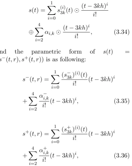
Figure 1: Approximate solution for case(i) in ex-ample4.1. Red points: s0(t); Green points: s3(t);
Blue. points: s6(t)
4
Numerical Example
Example 4.1 [20] Let us consider the following second-order fuzzy initial value problem
y′′(t) =σ0, y0 =γ0, y′(0) =γ1, (4.40)
where σ0 =γ0 =γ1 are the triangular fuzzy num-ber having r-level sets [r−1,1−r].
Case(i) Ify(t) is [(i)−gH]-differentiable, the real solution is:
y−(t, r) = (r−1){t 2
2 +t+ 1},
y+(t, r) = (1−r){t 2
2 +t+ 1},
Now we use PWA method to obtain piecewise ap-proximate solutions(t). LetIk = [kH,(k+ 1)H], for k= 0,1,2, H = 3h and h = 0.1. s0(t), s3(t)
and s6(t) are obtained as follows:
s−0(t) = (r−1) +t(r−1) + t 2
2(r−1),
s+0(t) = (1−r) +t(1−r)t+t 2
2(1−r), s−3(t) = 1.345r−1.345
+ (t−0.3)(1.3r−1.3)
+ (t−0.3) 2
2 (r−1), s+3(t) = 1.345−1.345r
+ (t−0.3)(1.3−1.3r)
+ (t−0.3) 2
2 (1−r), s−6(t) = 1.78r−1.78
+ (t−0.6)(1.6r−1.6)
+ (t−0.6) 2
2 (r−1), s+6(t) = 1.78−1.78r
+ (t−0.6)(1.6−1.6r))
+ (t−0.6) 2
2 (1−r),
The approximate solution si(t) in Case(i), for i= 0,1,2, is plotted in Fig 1.
Case(ii)If y(t) is [(ii) − gH]-differentiable, the real solution is:
y−(t, r) = (r−1){t 2
2 −t+ 1},
y+(t, r) = (1−r){t 2
in this case s0(t),s3(t) ands6(t) are obtained as follows:
s−0(t) = (r−1) +t(1−r) +t 2
2(r−1),
s+0(t) = (1−r) +t(r−1)t+t 2
2(1−r), s−3(t) = .745r−.745 + (t−0.3)(0.7−.7r)
+ (t−0.3) 2
2 (r−1),
s+3(t) = .745−.745r+ (t−0.3)(0.7r−.7)
+ (t−0.3) 2
2 (1−r),
s−6(t) = .58r−.58 + (t−0.6)(.4−.4r)
+ (t−0.6) 2
2 (r−1),
s+6(t) = .58−.58r+ (t−0.6)(.4r−.4r)
+ (t−0.6) 2
2 (1−r),
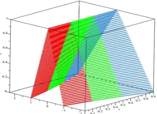
The approximate solutionsi(t) in Case(ii), fori= 0,1,2, is plotted in Fig 2.
Example 4.2 [20] Consider the fuzzy initial value problem
y′′(t) +y(t) =σ0, y(0) =γ0, y′(0) =γ1,
where σ0 is the fuzzy number having r-level sets [r,2−r]. [γ0]r= [γ1]r= [r−1,1−r].
Case(i) Ify(t) is [(i)−gH]-differentiable, the real solution is:
y−(t, r) = r(1 + sin(t))−sin(t)−cos(t),
y+(t, r) = (2−r)(1 + sin(t))
− sin(t)−cos(t),
Let Ik = [kH,(k+ 1)H],for k= 0,1,2,H = 3h and h = 0.1. s0(t), s3(t) and s6(t) are obtained
as follows:
s−0(t) = (r−1) +t(r−1)
+ t 2
2(.9992 + 0.00099r)
+ t 3
3!(1.016−1.01817r)
+ t 4
4!(−1.1778 +.1986r), s+0(t) = (1−r) +t(1−r)
+ t 2
2(1.001−0.00099r)
+ t 3
3!(−1.021 + 1.0182r)
+ t 4
4!(−.7807−.1985r), s−3(t) = (1.295r−1.2509)
+ (t−0.3)(.9554r−.6599)
+ (t−0.3) 2
2 (1.251−.2947r)
+ (t−0.3) 3
3! (.6688−.972r)
+ (t−0.3) 4
4! (−1.356 +.4791), s+3(t) = (1.3402−1.296r)
+ (t−0.3)(1.2509−.9554r)
+ (t−0.3) 2
2 (.6612 +.2946r)
+ (t−0.3) 3
3! (−1.275 +.972r)
+ (t−0.3) 4
4! (−.3978−.4791r), s−6(t) = (1.565r−1.39)
+ (t−0.6)(.8254r−.2608)
+ (t−0.6) 2
2 (1.39−.564r)
+ (t−0.6) 3
3! (.26201−.839r)
+ (t−0.3) 4
4! (−1.413 +.7169r), s+6(t) = (1.74−1.565r)
+ (t−0.6)(1.3901−.8254r)
+ (t−0.6) 2
2 (.26208 +.56394r)
+ (t−0.6) 3
3! (−1.416 +.839r)
+ (t−0.3) 4
The approximate solution si(t) in Case(i), for i= 0,1,2, is plotted in Fig 3.
Case(ii)If y(t) is [(ii) − gH]-differentiable, the real solution is:
Figure 2: Approximate solution for case(ii) in ex-ample4.1. Red points: s0(t); Green points: s3(t);
Blue points: s6(t)
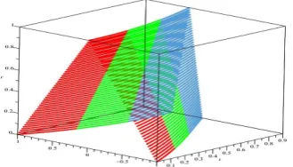
Figure 3: Approximate solution for case(ii) in ex-ample 4.2. Red points: s0(t); Green points:s3(t);
Blue points: s6(t)
Figure 4: Approximate solution for case(i) in ex-ample4.2. Red points: s0(t); Green points: s3(t);
Blue points: s6(t)
y−(t, r) =r(1−sin(t)) + sin(t)−cos(t),
y+(t, r) = (2−r)(1−sin(t))
+ sin(t)−cos(t),
s0(t), s3(t) ands6(t) are obtained as follows:
s−0(t) = (r−1) +t(1−r)
+ t 2
2(1.0011−0.00099r)
+ t 3
3!(−1.021 + 1.0182r)
+ t 4
4!(−.78074−.19851r), s+0(t) = (1−r) +t(r−1)
+ t 2
2(.9992 + 0.00099r)
+ t 3
3!(1.0157−1.01818r)
+ t 4
4!(−1.1778 +.1985r), s−3(t) = (.7045r−.6599)
+ (t−0.3)(1.251−.95537r)
+ (t−0.3) 2
2 (.66114 +.2946r)
+ (t−0.3) 3
3! (−1.7527 +.97199r)
+ (t−0.3) 4
4! (−.3978−.4791r), s+3(t) = (.7492−.70447r)
+ (t−0.3)(.9554r−.65985)
+ (t−0.3) 2
2 (1.2504−.29463r)
+ (t−0.3) 3
3! (.66872−.97199r)
+ (t−0.3) 4
4! (−1.3559 +.47905r), s−6(t) = (.43533r−.26066)
+ (t−0.6)(1.3901−.825399r)
+ (t−0.6) 2
2 (.26207 +.56394r)
+ (t−0.6) 3
3! (−1.41597 +.83899r)
+ (t−0.3) 4
4! (0.0207−.71680r), s+6(t) = (.610−.43533r)
+ (t−0.6)(.8254r−.26074)
+ (t−0.6) 2
2 (1.3899−.56394r)
+ (t−0.6) 3
3! (.26201−.838989r)
+ (t−0.3) 4
The approximate solutionsi(t) in Case(ii), fori= 0,1,2, is plotted in Fig 4.
5
Conclusion
In this paper a new approach for solving sec-ond order fuzzy differential equations under gen-eralized differentiability was proposed. We used piecewise fuzzy polynomial of degree 4 based on the Taylor expansion for approximating solutions of second order fuzzy differential equations. Also, we can develop this method for Nth-order fuzzy differential equations under generalized deriva-tives.
6
Acknowledgments
The authors are grateful to the Islamic Azad Uni-versity, Shahr-e-Qods branch for infinite support and grant.
References
[1] S. Abbasbandy, T. Allahviranloo, Numer-ical Solutions of Fuzzy Differential Equa-tions By Taylor Method, Journal of Com-putational Methods in Applied Mathematics 2 (2002) 113-124.
[2] T. Allahviranloo, N. Ahmady, E.Ahmady, Numerical solution of fuzzy differential equations by Predictor-Corrector method, Information Sciences177 (2007) 1633-1647.
[3] T. Allahviranloo, E. Ahmady, N. Ah-mady, Nth-order fuzzy linear differential equations,Information Sciences178 (2008) 1309-1324.
[4] T. Allahviranloo, E. Ahmady, N. Ah-mady, A method for solving nth order fuzzy linear differential equations, Inter-national Journal of Computer Mathemat-ics11 (2009) 730-742http://dx.doi.org/ 10.1080/00207160701704564/.
[5] T. Allahviranloo, S. Abbasbandy, N. Ah-mady, E. AhAh-mady, Improved predictor-corrector method for solving fuzzy initial value problems, Information Sciences 179 (2009) 945-955.
[6] Allahviranloo, Z. Gouyandeh, A. Armand, A full fuzzy method for solving differen-tial equation based on Taylor expansion, Journal of Intelligent and Fuzzy Systems 29 (2015) 10391055 http://dx.doi.org/10. 3233/IFS-151713./.
[7] M.R. Balooch Shahryari, S. Salahshour, Improved predictor-corrector method for solving fuzzy differential equations un-der generalized differentiability, Journal of Fuzzy Set Value Analysis 2012 (2012) 1-16.
[8] B. Bede, I. J. Rudas, A. L. Bencsik, First order linear fuzzy differential equations un-der generalized differentiability, Informa-tion Sciences 177 (2007) 1648-1662.
[9] B. Bede, S. G. Gal, Generalizations of the differentiability of fuzzy-number-valued functions with applications to fuzzy differ-ential equations,Fuzzy Set and Systems151 (2005) 581-599.
[10] B. Bede, S. G. Gal, Remark on the new solutions of fuzzy differential equations, Chaos Solitons Fractals (2006).
[11] B. Bede, L. Stefanini, Solution of Fuzzy Dif-ferential Equations with generalized differ-entiability using LU-parametric representa-tion,EUSFLAT 1 (2011) 785-790.
[12] B. Bede, L. Stefanini, Generalized differ-entiability of fuzzy-valued functions, Fuzzy Sets and Systems 230 (2013) 119-141.
[13] J. J. Buckley, T. Feuring, Fuzzy initial value problem for Nth-order linear differen-tial equations, Fuzzy Sets and System 121 (2001) 247-255.
[14] S. L. Chang, L. A. Zadeh, On fuzzy map-ping and control, IEEE Trans, Systems Man Cybernet 2 (1972) 30-34.
[15] D. Dubois, H. Prade, Towards fuzzy dif-ferential calculus: Part 3, differentiation, Fuzzy Sets and Systems 8 (1982) 225-233.
[17] M. Friedman, M. Ma, A. Kandel, Numeri-cal solutions of fuzzy differential and inte-gral equations,Fuzzy Sets and Systems 106 (1999) 35-48.
[18] D. N. Georgiou, J. J. Nieto, R. Rodriguez-Lopez, Initial value problems for higher-order fuzzy differential equations, Nonlin-ear Analysis: Theory, Methods and Appli-cations 63 (2005) 587-600.
[19] O. Kaleva, Fuzzy differential equations, Fuzzy Sets Syst. 24 (1987) 319-330.
[20] A. Khastan, F. Bahrami, K. Ivaz, New Re-sults on Multiple solution for Nth-Order Fuzzy Differential Equations under Gen-eralized Differentiability, Boundary Value Problems, 2009 (2009) 1-13.
[21] M. Ma, M. Friedman, A. Kandel, Numeri-cal Solutions of fuzzy differential equations, Fuzzy Sets and Systems105 (1999) 133-138.
[22] S. Sallam, H. M. El-Hawary, A deficient spline function approximation to system of first order differential equations, App. Math. Modelling 7 (1983) 380-382.
[23] S. Seikkala, On the fuzzy initial value prob-lem,Fuzzy Sets and Systems 24 (1987) 319-330.
Elham Ahmady has got PhD de-gree from Islamic Azad University Science and Research Branch in 2008 She has been member of the faculty in Islamic Azad University Shahr-e-Qods branch since 2005. Main research interest include: Fuzzy differential equations, Ranking and fuzzy systems.