On the Roots of Hosoya Polynomial of a Graph

On the roots of Hosoya polynomial of a graph

M.H.REYHANIa,S.ALIKHANIb,M.A.IRANMANESHb

a

Department of Mathematics, Yazd Branch, Islamic Azad University, Yazd, Iran b

Department of Mathematics, Yazd University, 89195-741, Yazd, Iran

(ReceivedAugust 10, 2013; Accepted August 20, 2013)

ABSTRACT

Let G = (V, E) be a simple graph. Hosoya polynomial of G is )

v , u ( d ) G ( V } v , u

{ x

= ) x , G (

H  _ , where, d(u ,v) denotes the distance between vertices u

and v. As is the case with other graph polynomials, such as chromatic, independence and domination polynomial, it is natural to study the roots of Hosoya polynomial of a graph. In this paper we study the roots of Hosoya polynomials of some specific graphs.

Keywords: Hosoya polynomial, root, path, cycle.

1.

I

A simple graph G = ( V, E ) is a finite nonempty set V(G) of objects called vertices together with a (possibly empty) set E(G) of unordered pairs of distinct vertices of G called edges. In chemical graphs, the vertices of the graph correspond to the atoms of the molecule, and the edges represent the chemical bonds.

The Hosoya polynomial of a graph is a generating function about distance distributing, introduced by Hosoya [10] in 1988 and for a connected graph G is defined as:

, x

= ) x , G (

H d(u,v)

) G ( V } v , u {





Where d (u ,v) denotes the distance between vertices u and v. This polynomial has computed for some nano-structures, e.g. [3, 16]. The Hosoya polynomial has many chemical applications [7, 8, 9]. Especially, the two well-known topological indices, i.e. Wiener index and hyper-Wiener index, can be directly obtained from the Hosoya polynomial.

The Wiener index of a connected graph G is denoted by W(G), is defined as the

). v , u ( d = ) x , G ( W ) G ( V } v , u {  

The hyper-Wiener index is denoted by WW(G) and defined as follows:

). v , u ( d 2 1 ) v , u ( d 2 1 = ) G ( WW 2 ) G ( V } v , u { ) G ( V } v , u {     

Note that the first derivative of the Hosoya polynomial at x=1 is equal to the Wiener index: . | ) ) x , G ( H ( = ) G (

W  _x=1

Also we have the following relation:

. | ) ) x , G ( xH ( 2 1 = ) G (

WW  _x=1

Graph polynomials are a well-developed area useful for analyzing properties of graphs. For some graph polynomials, their roots have attracted considerable attention, both for their own sake, as well for what the nature and location of the roots imply. Woodal [17] explored the zeros and zero-free regions of chromatic and flow polynomials. Also, the zero distribution of chromatic and flow polynomials of graphs and characteristic polynomials of matroids have been examined by Jackson [12]. Also the zeros of independence polynomials have been studied in [2, 4]. Finally the roots of domination polynomial has considered in some papers, e.g. [1, 5].

In this paper we study the roots of Hosoya polynomial of specific graphs. We denote the roots of Hosoya polynomial of graph G by Z(H(G,x)).

2.

M

R

In this section we consider some specific graphs and obtain the roots of their Hosoya polynomials. Let S_n,P_n and C denote the star, path and cycle with _n n vertices,

respectively. A simple calculation gives the following theorem:

Theorem 1.

1. x (n 1)x.

2 1 n = ) x , S (

H _{n } 2  

     

2. H(P_n,x)=xn12xn2...(n1)x.

3. H(C_2n,x)=(2n)(xx2xn1)nxn.

Theorem 2 . For n3,

}. n 2

2 {0, = )) x , S ( H (

Z _n



Proof. It follws from Theorem 1(i). ■

Here we state the following theorem:

Theorem 3 . ([14]) Let f(z)=a_nzn a_n1zn1a₀, a_iR,i=1,,n be a

polynomial with real coefficients satisfying a₀a₁a_n >0. Then, no zeros of f(z)

lie in {zC,|z|<1}.

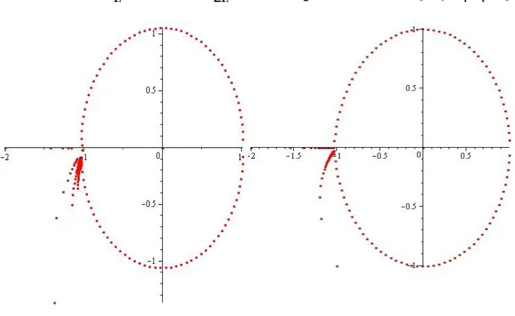
The following theorem is an consequence of Theorem 3, see Figure 1.

Theorem 4 . H(P_n,x) and H(C_2n,x) do not possess zeros in {zC,|z|<1}.

Figure 1. Roots of Hosoya polynomial of P₁₀₀ and C₂₀₀, respectively.

We recall that the n-th root of unity are roots n i k 2

e 

of equation xn 1. Now we state and prove the following theorem:

Theorem 5 . Let f(z)=azn azn1aza, a0, be a complex polynomial. All

zeros of f(z) lie on the unit circle.

), w z ( a = 1 z

1) z

( a = ) z (

f n i

1 = i 1

n

  





where w denotes the (n1)-th root of unity. Since all roots of unity lie on the unit circle,

so we have the result. ■

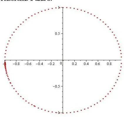
Corollary 1: All roots of H(C_2n1,x)lie on the unit circle.

Proof. It follows from Theorems 1 and 5. ■

Figure 2. Roots of H(C₂₀₁,x).

Figure 2 shows roots of H(C₂₀₁,x). We need the following theorem:

Theorem 6 . ([13]) Let f(z)=a_nzn a_n1zn1a₀, a_iR, be a polynomial with real coefficients. All zeros of f(z) lie in the closed disk {zC,|z|r} where r>1 denotes

the largest positive root of the equation (z21)(|a_n|z|a_n1|)222₂ =0, and

2 1 2 1 j n j n n

1 = j

2 ( (a a ) )

2 1

=  _  _{ }

 .

Theorem 7. All zeros of H(C_2n,x) lie in the closed disk {zC,|z|2.77321}.

Proof. By Theorem 6, since we have a_n =n and a_i = 2n, (1in1), so ₂ = 2n.

2.77321. So, we have the result as desired. ■

The join G₁G₂ of two graph G₁ and G with disjoint vertex sets ₂ V₁ and V a₂ nd

edge sets E and ₁ E is the graph union ₂ G₁G₂ together with all the edges joining V and ₁

2 V .

Theorem 8 . Let n and _i m be order and size of graphs _i G i (i=1,2), respectively. Then

. ) m m ( 2 n 2 n n n m m 0, = )) x , G G ( H ( Z 2 1 2 1 2 1 2 1 2 1                                 

Proof. Since H G G x m n_ x  E G  E G x x mnx

           

 ) (| ( )| | ( )|) ( 1) 2 2 ( = ) ,

( 1 2

2 2

1 (see

[15]), we have the result. ■

The following corollary is an immediate consequence of Theorem 8:

Corollary 2.

1. The roots of Hosoya polynomial of complete bipartite graph K_m,n is

. 2 m 2 n mn 0, = )) x , K ( H (

Z _m,n

                           

2. The roots of Hosoya polynomial of wheel graph W_n is

. 1) n ( 2 1 n n 2 2 0, = )) x , W ( H ( Z _n                         Proof.

1. Since K_m,n =K_mK_n , we have the result by Theorem 8.

2. Since W_n =K₁C_n1, we have the result by Theorem 8. ■

composition) of G and H, and can be thought of as the graph arising from G and H by substituting a copy of H for every vertex of G. We need the following theorem:

Theorem 9. ([15]) Let G₁ and G₂ be two graphs of order m and n, respectively. The

Hosoya polynomial of G₁[G₂] is

1) x ( x | ) G ( E | m x 2 n m ) x , G ( H n = ) x ], G [ G (

H _{1 2} 2 _{1 } 2 ₂ 

     

Corollary 3. Let G₁ and G₂ be two graphs of order m and n , respectively. The only

common root of H(G₁,x) and H(G₁[G₂],x) is

      

2 n | ) G ( E |

| ) G ( E |

2

2 _.

Proof. Let  be a common root of H(G₁,x) and H(G₁[G₂],x). Therefore by Theorem 9

we have |E(G )| = |E(G )| 2

n

2 2 _ 

  

  

      

. So we have the result. ■

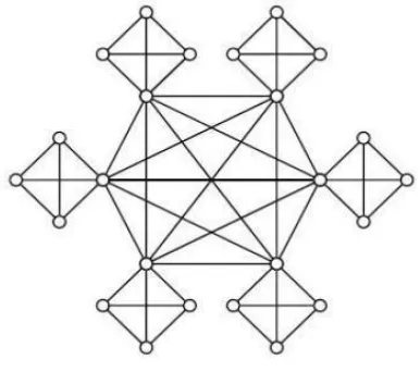
Here we shall consider the roots of Hosoya polynomial of another specific graph. Consider the graph K_m and m copies of K . The graph _n Q(m,n) is obtained by

identifying each vertex of K_m with a vertex of a unique K (see [6]). We have shown the _n

graph Q(6,4) in Figure 3.

Figure 3. Q(6,4).

3 2 2

2 _{m(m 1)(n 1) x}

2 1 x 1) n 1)( m ( m x 1) n n m ( m 2 1

  

  

  

The following theorem is about roots of Hosoya polynomial of Q(m,n):

Theorem 11 . All non-zero roots of H(Q(m,n),x) are complex.

Proof. By Theorem 10 we have the following equation:

0. = 1) n n m ( x 1) n 1)( m 2( x 1) n 1)( m

(   2 2      2  

It is easy to see that =4n(n1)3(m1), where is the discriminant of the quadratic

equation. Since m,nN, we have <0. Therefore we have the result. ■

We have seen that there are graphs whose their nonzero roots of Hosoya polynomial are complex. We think that the following problem has worth to consider:

Problem. Characterize graphs whose nonzero roots of their Hosoya polynomial have are complex.

A

The authors would like to express their gratitude to the referee for her/his careful reading and helpful comments.

R

1. S. Akbari, S. Alikhani, M. R. Oboudi and Y.H. Peng, On the zeros of domination polynomial of a graph, Contemporary Mathematics, American Mathematical Society, 531 (2010) 109115.

2. S. Alikhani, Y.H. Peng, Independence roots and independence fractals of certain graphs, J. Appl. Math. Computing, vol. 36, no. 1-2 (2011) 89100.

3. C. Eslahchi, S. Alikhani, M.H. Akhbari, Hosoya polynomial of an infinite family of dendrimer nanostar, Iran. J. Math. Chem. Vol. 2, No. 1 (2011) 7179.

4. J. I. Brown, C.A. Hickman, R.J. Nowakowski, On the location of roots of independence polynomials. J. Algebr. Comb. 19 (2004) 273–282.

5. J. Brown and J. Tufts, On the roots of domination polynomials, Graphs Combin., (2013) DOI 10.1007/s00373-013-1306-z.

subgraphs, arXiv:1212.3179v1 [math.CO].

7. E. Estrada, O. Ivanciuc, I. Gutman, A. Gutierrez, L. Rodrguez, Extended Wiener Indices. A New Set of Descriptors for Quantitative Structure-Property Studies, New J. Chem., 22 (1998) 819823.

8. I. Gutman, S. Klavzar, M. Petkovsek, P. Zigert, On Hosoya polynomials of benzenoid graphs, MATCH Commun. Math. Comput. Chem., 43 (2001) pp. 4966. 9. I. Gutman, Y. Zhang, M. Dehmer, A.Ilic, Altenburg, Wiener, and Hosoya

Polynomials, preprint.

10.H. Hosoya, On some counting polynomials in chemistry, Discrete Appl. Math., 19

(1988) pp. 239257.

11.H. Hosoya, A Newly Proposed Quantity Characterizing the Topological Nature of Structural Isomers of Saturated Hydrocarbons, Bull. Chem. Soc. Japan 44 (1971) 23322339.

12.B. Jackson, Zeros of chromatic and ow polynomials of graphs, J. Geometry 76

(2003) 95109.

13.S. Kakeya, On the limits of the roots of an algebraic equation with positive coefficients. Tôhoku Math. J., 2 (1912) 140–142.

14.V.V. Prasolov, Polynomials, Springer- Verlag Berlin Heidelberg, (2004).

15.D. Stevanović, Hosoya polynomial of composite graphs, Discrete Math. 235 (2001) 237244.

16.S. Xu and H. Zhang, Hosoya polynomials of TUC₄C₈(S) nanotubes, J. Math.

Chem., 45 (2009) 488–502.