The Thirty-Third AAAI Conference on Artificial Intelligence (AAAI-19)
A Nonconvex Projection Method for Robust PCA
Aritra Dutta,
∗Filip Hanzely,
†Peter Richt´arik
‡Abstract
Robust principal component analysis (RPCA) is a well-studied problem whose goal is to decompose a matrix into the sum of low-rank and sparse components. In this paper, we propose a nonconvex feasibility reformulation of RPCA problem and apply an alternating projection method to solve it. To the best of our knowledge, this is the first paper proposing a method that solves RPCA problem without considering any objective function, convex relaxation, or surrogate convex constraints. We demonstrate through extensive numerical experiments on a variety of applications, including shadow removal, background estimation, face detection, and galaxy evolution, that our ap-proach matches and often significantly outperforms current state-of-the-art in various ways.
Principal component analysis (PCA) (Jolliffee 2002) ad-dresses the problem of best approximation of a matrix A∈Rm×nby a matrix of rankr:
X∗= arg min
X∈Rm×n
rank(X)≤r
∥A−X∥2
F, (1)
where∥ · ∥F denotes the Frobenius norm of matrices. The
solution to (1) is given by
X∗=Hr(A) def
=UΣrVT, (2)
whereA has singular value decompositionsA = UΣVT,
andΣr(A)is the diagonal matrix obtained fromΣby
hard-thresholding that keeps therlargest singular values only and
∗
Aritra Dutta is with the Visual Computing Center, Divi-sion of Computer, Electrical and Mathematical Sciences and Engineering (CEMSE) at King Abdullah University of Science and Technology, Thuwal, Saudi Arabia-23955-6900, e-mail: [email protected].
†
Filip Hanzely is with the Visual Computing Center, Divi-sion of Computer, Electrical and Mathematical Sciences and Engineering (CEMSE) at King Abdullah University of Sci-ence and Technology, Thuwal, Saudi Arabia-23955-6900, e-mail: [email protected].
‡
Peter Richt´arik is with the Visual Computing Center, Di-vision of Computer, Electrical and Mathematical Sciences and Engineering (CEMSE) at King Abdullah University of Science and Technology, University of Edinburgh, and MIPT, e-mail: [email protected].
Copyright c⃝2019, Association for the Advancement of Artificial Intelligence (www.aaai.org). All rights reserved.
replaces the other singular values by 0. In many real-world problems, if sparse large errors or outliers are present in the data matrix, PCA fails to deal with it. Therefore, it is natural to consider arobustmatrix decomposition model in which we wish to decomposeAinto the sum of a low-rank matrixL and an error matrixS:A=L+S. However, without further assumptions, the problem is ill-posed. We assume that the error matrixSissparseand that it allows its entries to have arbitrarily large magnitudes. That is, givenA, we consider the problem of finding a low rank matrix Land a sparse matrixSsuch that
A=L+S. (3)
In this context, the celebrated principal component pursuit (PCP) formulation of the problem uses theℓ0norm
(cardinal-ity) to address the sparsity constraint and (3). Therefore, PCP is the constrained minimization problem (Cand`es et al. 2011; Chandrasekaran et al. 2011):
min
L,S rank(L) +λ∥S∥ℓ0 subject to A=L+S, (4)
whereλ >0is a balancing parameter. Since bothrank(L)
and∥S∥ℓ0 are non-convex, one often replaces the rank
func-tion by the (convex) nuclear norm andℓ0by the (convex)
ℓ1norm. This replacement leads to the immensely popular
robust principal component analysis (RPCA)(Wright et al. 2009; Lin, Chen, and Ma 2010; Cand`es et al. 2011), which can be seen as a convex relaxation of (4):
min
L,S ∥L∥∗+λ∥S∥ℓ1 subject to A=L+S, (5)
where∥ · ∥∗denotes the nuclear norm (sum of the singular
Yang (Zhang and Yang 2017) proposed a manifold optimiza-tion to solve RPCA. We refer the reader to (Bouwmans and Zahzah 2014) for a comprehensive review of the RPCA al-gorithms. However, besides formulation (5), other tractable reformulations of (4) exist as well. For instance, by relaxing the equality constraint in (4) and moving it to the objective as a penalty, together with adding explicit constraints on the target rankrand target sparsitysleads to the following formulation (Zhou and Tao 2011):
minL,S∥A−L−S∥2F
subject to rank(L)≤r and ∥S∥0≤s. (6)
One can extend the above model to the case of partially observed data that leads to the robust matrix completion (RMC) problem (Chen et al. 2011; Tao and Yang 2011; Cherapanamjeri, Gupta, and Jain 2017):
minL,S∥PΩ(A−L−S)∥2F
subject to rank(L)≤r and ∥PΩ(S)∥0≤s′, (7)
whereΩ⊆[m]×[n]is the set of observed data entries, and
PΩis the restriction operator defined by
(PΩ[X])ij = {
Xij (i, j)∈Ω
0 otherwise.
We note that with some modifications, problem (6) is con-tained in the larger class of problem presented by (7). We also refer to some recent work on RMC problem or outlier based PCA in (Cherapanamjeri, Jain, and Netrapalli 2017; Cherapanamjeri, Gupta, and Jain 2017). An extended model of (5) can also be referred to as a more general problem as in (Tao and Yang 2011) (see problem (1.2) in (Tao and Yang 2011)). More specifically, whenΩ = [m]×[n], that is, the whole matrix is observed, then (7) is (6). One can also think of the matrix completion (MC) problem as a special case of (7) (Cand`es and Plan 2009; Jain, Netrapalli, and Sanghavi 2013; Cai, Cand`es, and Shen 2010; Jain and Netrapalli 2015; Cand`es and Recht 2009; Keshavan, Montanari, and Oh 2010; Cand`es and Tao 2010; Mareˇcek, Richt´arik, and Tak´aˇc 2017). For MC problems,S= 0. Therefore, (7) is a generalization of two fundamental problems: RPCA and RMC.
Contributions.We solved the RPCA and RMC problems by addressing the original decomposition problem (3) di-rectly, without introducing any optimization objective or sur-rogate constraints. This is a novel approach because we aim to find a point at the intersection of three sets, two of which are non-convex. We formulate both RPCA and RMC as set feasibility problems and propose alternating projection algo-rithm to solve them. This leads to Algoalgo-rithm 2 and 3. Our approach is described in the next section. We also propose a convergence analysis of our algorithm.
Our feasibility approach does not require one to use the hard to interpret parameters (such asλ) and surrogate func-tions (such as the nuclear norm, orℓ1norm) which makes
our approach unique compared to existing models. Instead, we rely on two direct parameters: the target rankrand the desired level of sparsitys. By performing extensive numeri-cal experiments on both synthetic and real datasets, we show that our approach can match or outperform state-of-the-art
methods in solving the RPCA and RMC problems. More precisely, when the sparsity level is low, our feasibility ap-proach can viably reconstruct any target low rank, which the RPCA algorithms can not. Moreover, our approach can tolerate denser outliers than can the state-of-the-art RPCA algorithms when the original matrix has a low-rank structure (see details in the experiment section). These attributes make our approach attractive to solve many real-world problems because our performance matches or outperforms that of state-of-the-art RPCA algorithms in solution quality, and do this in comparable or less time.
Nonconvex Feasibility and Alternating
Projections
Set feasibility problem aims to find a point in the intersection of a collection of closed sets, that is:
Find x∈ X where X def=∩m
i Xi̸=∅, (8)
for closed setsXi. Usually, setsXis are assumed to be simple
and easy to project on. A special case of the above setting for convex setsXiis the convex feasibility problem and is already
well studied. In particular, a very efficient convex feasibility algorithm is known as the alternating projection algorithm (Kaczmarz 1937; Bauschke and Borwein 1996), in which each iteration picks one setXiand projects the current iterate
on it. There are two main methods to choosing the setsXi–
traditional cyclic method and randomized method (Strohmer and Vershynin 2009; Gower and Richt´arik 2015; Necoara, Richt´arik, and Patrascu 2018), and in general, randomized method is faster and not vulnerable to adversarial set order.
We also note that the alternating projection algorithm for convex feasibility problem does not converge in general to the projection of the starting point ontoX, but rather finds a close-to feasible point in X, except the case whenXis
are affine spaces. However, once an exact projection onto
X is desired, Dykstra’s algorithm (Boyle and Dykstra 1986) should be applied.
Algorithm 1:Alternating projection method for set fea-sibility
1 Input :Πi(·)– Projector ontoXifor each
i∈ {1, . . . m}, starting pointx0
2 fork= 0,1, . . . do
3 Choose via some rulei(e.g., cyclically or randomly)
4 xk+1= Πi(xk)
end
5 Output :xk+1
On the other hand, for general nonconvex setsXi,
Set feasibility for RPCA
In this scope, we defineα-sparsity as it appears in the last convex constraintX3. We do it so that our approach is directly
comparable to the approaches from (Yi et al. 2016; Zhang and Yang 2017). However, we note that theℓ0-ball constraint
can be applied as well.
Definition 1(α-sparsity). A matrixS ∈ Rm×nis
consid-ered to beα-sparse if each row and column ofScontains at mostαnandαmnonzero entries, respectively. That is, the cardinality of the support set of each row and column of the matrixSdo not exceedαnandαm, respectively. Formally, we write
∥S(i,.)∥0≤αn and ∥S(.,j)∥0≤αm for alli∈[m], j∈[n],
where ith row andjth column ofS areS
(i,.)and S(.,j),
respectively.
Now we consider the following reformulation of RPCA:
Find M def= [L, S]∈ X def=∩3
i=1Xi̸=∅, (9)
where
X1
def
= {M|L+S=A} (10)
X2
def
= {M|rank(L)≤r}
X3
def
= {M| ∥S(i,.)∥0≤αn and ∥S(.,j)∥0≤αm
for alli∈[m], j∈[n].}
Clearly,X1is convex, butX2 andX3are not.
Neverthe-less, the algorithm we propose – alternating Frobenius norm projection onXi performs well to solve RPCA in practice.
To validate the robustness of our algorithm, we compare our method to other state-of-the-art RPCA approaches on vari-ous practical problems. We also study the local convergence properties and show that despite the non-convex nature of the problem, the algorithms we propose often behave surprisingly well.
The Algorithm
DenoteΠi to be projector ontoXi. Note thatΠ2 does not
includeSand projection ontoΠ3does not includeL.
Con-sequently,Π2Π3is a projector ontoX2∩ X3. Because our
goal is to find a point at the intersection of two sets, we shall employ a cyclic projection method (note that random-ized method does not make sense). Indeed, steps 4 and 5 of Algorithm 2 perform projection ontoX1, step 6 performs
projection ontoX2, and finally, step 7 performs projection
ontoX3. Later in this section we describe the exact
imple-mentation and prove correctness the steps mentioned above. Lastly, we propose a similar algorithm to solve the RMC problem (7) in Appendix (Algorithm 3). Finally, we provide a local convergence of Algorithm 2, which depends on the local geometry of the optimal point, and is mostly linear, which we prove later.
Projection on the linear constraint. The next lemma pro-vides an explicit formula for the projection ontoX1, which
corresponds to steps 4 and 5 of Algorithm 2.
Algorithm 2:Alternating projection method for RPCA
1 Input :A∈Rm×n(the given matrix), rankr,
sparsity levelα∈(0,1]
2 Initialize :L0, S0
3 fork= 0,1, . . . do 4 L˜ =12(Lk−Sk+A)
5 S˜= 1
2(Sk−Lk+A)
6 Lk+1=Hr( ˜L)
7 Sk+1=Tα( ˜S)
end
8 Output :Lk+1, Sk+1
Lemma 1. Solutions to
min
L,S∥L−L0∥ 2
F+∥S−S0∥2F subject to L+S=A
isL∗= 12(L0−S0+A)andS∗= 12(S0−L0+A).
Projection on the low rank constraint. ConsiderL(r)to be the projection ofLonto the rankrconstraint, that is,
L(r)= arg min
L′ ∥L ′−L∥
F subject to rank(L′)≤r.
It is known that L(r) can be computed as r-SVD ofL.
Fast r-SVD solvers has improved greatly in recent years (Halko, Martinsson, and Tropp 2011; Musco and Musco 2015; Shamir 2015; A.-Zhu and Li 2016). Unfortunately, the most recent approaches (Shamir 2015; A.-Zhu and Li 2016) were not applied in our setting because they are inefficient; they need to computeLL⊤(orL⊤L), which is expensive. Instead, we use block Krylov approach from (Musco and Musco 2015). For completeness, we quote the algorithm in Appendix. Regarding the computational complexity, it was shown that block Krylov SVD outputsZ satisfying ∥L−
ZZ⊤L∥F ≤(1 + ˜ϵ)∥L−L(r)∥F in
O
(
∥L∥0
rlogn
√
˜
ϵ +
mr2log2n
˜
ϵ +
r3log3n
˜
ϵ3/2 )
flops. Therefore, projection on the low-rank constraint is not an issue for relatively small rankr.
Projection on sparsity constraint. Projection onto X3
simply keeps theα-fraction of the largest elements in ab-solute value in each row and column and set the rest to zero. One can use a global hard-thresholding operator that consid-ersℓ0constraint on the entire matrix. Instead, we proposed
an operatorTα(·). Indeed,Tα(·)does not perform an explicit
Euclidean projection ontoX3. Instead, it performs a
projec-tion onto a certain subset ofX3 and this is clear from the
definition (11) (the subset is defined through supportΩα).
Formally, we define:
Tα[S]
def
= PΩα(S)∈R
m×n: (i, j)∈Ω αif
|Sij| ≥ |S
(αn)
(i,.)| and|Sij| ≥ |S
0.1 0.2 0.3 0.4 0.5 0.6 0.7 0.8 0.9 1 0 0.1 0.2 0.3 0.4 0.5 0.6 0.7 0.8 0.9 1 (a)
0.1 0.2 0.3 0.4 0.5 0.6 0.7 0.8 0.9 1 0 0.1 0.2 0.3 0.4 0.5 0.6 0.7 0.8 0.9 1 (b)
0.1 0.2 0.3 0.4 0.5 0.6 0.7 0.8 0.9 1 0 0.1 0.2 0.3 0.4 0.5 0.6 0.7 0.8 0.9 1 (c)
0.1 0.2 0.3 0.4 0.5 0.6 0.7 0.8 0.9 1 0 0.1 0.2 0.3 0.4 0.5 0.6 0.7 0.8 0.9 1 (d)
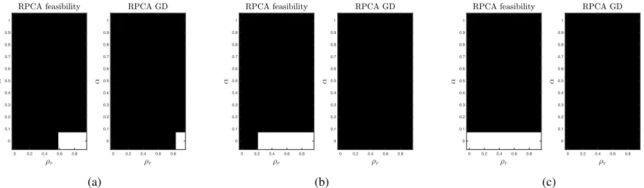
Figure 1: Phase transition diagram for RPCA F, iEALM, APG, and GoDec with respect to rank and error sparsity. Here, ρr = rank(L)/mandαis the sparsity measure. We have(ρr, α) ∈ (0.025,1]×(0,1) withr = 5 : 5 : 200and α = linspace(0,0.99,40). We perform 10 runs of each algorithm.
0 0.2 0.4 0.6 0.8 0 0.1 0.2 0.3 0.4 0.5 0.6 0.7 0.8 0.9 1
0 0.2 0.4 0.6 0.8 0 0.1 0.2 0.3 0.4 0.5 0.6 0.7 0.8 0.9 1 (a)
0 0.2 0.4 0.6 0.8 0 0.1 0.2 0.3 0.4 0.5 0.6 0.7 0.8 0.9 1
0 0.2 0.4 0.6 0.8 0 0.1 0.2 0.3 0.4 0.5 0.6 0.7 0.8 0.9 1 (b)
0 0.2 0.4 0.6 0.8 0 0.1 0.2 0.3 0.4 0.5 0.6 0.7 0.8 0.9 1
0 0.2 0.4 0.6 0.8 0 0.1 0.2 0.3 0.4 0.5 0.6 0.7 0.8 0.9 1 (c)
Figure 2: Phase transition diagram for Relative error for RMC problems: (a)|ΩC| = 0.5(m.n), (b) |ΩC| = 0.75(m.n), (c)|ΩC| = 0.9(m.n). Here, ρ
r = rank(L)/mandαis the sparsity measure. We have(ρr, α) ∈ (0.025,1]×(0,1)with
r= 5 : 25 : 200andα=linspace(0,0.99,8).
whereS((i,.αn))andS((.,jαm))denote theαfraction of largest en-tries ofSalong theithrow andjthcolumn, respectively. This
allows us to inexpensively compute an approximate projec-tion ontoX3which works well in practice. Remarkably, this
does not affect our theoretical results (which are formulated for exact projection ontoX3) in any way. We note that the
operatorTα(·)is similar to that defined in (Yi et al. 2016;
Zhang and Yang 2017). Projection on sparsity constraint (11) can be implemented inO(nd)time: for each row and each column we findαn-th largest element (orαd) and simul-taneously (for other rows/columns) mask the rest. In our experiments, we use fast implementation ofn-th element computation from (Li 2013).
Remark1. One may use the Douglas-Rachford operator split-ting method (Artacho, Borwein, and Tam 2016) as an alter-native to the nonconvex projections. We leave this for future research.
Convergence Analysis
In this section, we establish a local convergence analysis of our algorithm by using the basic properties of the alternating projection algorithm (Lewis and Malick 2008). A similar analysis was done for GoDec (Zhou and Tao 2011), although Algorithm 2 is vastly different compare to GoDec (we report detailed comparison of these algorithms in Appendix).
Recall that Algorithm 1 performs an alternating projection of[L, S]on the setsX1andX∩
def
=X2∩ X3defined in (10).
Before stating the convergence theorem, let us define a (local) angle between sets.
Definition 2. Let a pointpbe in the intersection of set bound-aries∂Kand∂L. Definec(K, L, p)be the cosine of an angle between setsKandLat point apas:
c(K, L, p)def= cos∠(∂K⊤|p, ∂L⊤|p),
where∂K⊤|pdenotes a tangent space of set boundary∂K
at pand∠returns the angle between subspaces given as arguments. As a consequence, we have0≤c(K, L, p)≤1. Let us also definedX1∩X∩(x)to be an Euclidean distance
of a pointxto the setX1∩ X∩.
Theorem 3. (Lewis and Malick 2008) Suppose that[ ¯L S¯]∈
∂(X1 ∩ X∩). Given any constantc ∈ R such that c >
c(X1,X∩,[ ¯L S¯])there is a starting point [L0 S0] close
to[ ¯L S¯]such that the iteratesLk, Skof Algorithm 2 satisfy
dX1∩X∩([Lk Sk])< c k
dX1∩X∩([L0 S0]).
Remark 2. From Theorem 3 it is clear that the smaller c(X1,X∩,[ ¯L S¯]) produces a faster convergence, while
c(X1,X∩,[ ¯L S¯]) = 1can stop the convergence, as described
BG+FG Ours RPCA GD iEALM APG Ours FG RPCA GD FG iEALM FG APG FG
Figure 3: Background and foreground separation on Stuttgart datasetBasicvideo. Except RPCA GD and our method, all other methods fail to remove the static foreground object.
Image:550
BG+FG
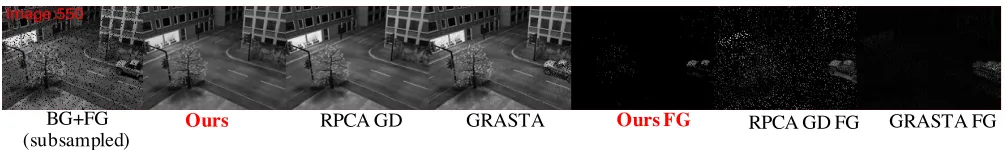
(subsampled) Ours RPCA GD GRASTA Ours FG RPCA GD FG GRASTA FG
Figure 4: Background and foreground separation on Stuttgart datasetBasicvideo. We used 90% sample. GRASTA forms a fragmentary background and exhausts around 540 frames to form a stable video. We also note that RPCA GD has more false positives in the foreground.
Remark3. Theorem 3 is stated for Algorithm 2, however, one can easily obtain an equivalent result for Algorithm 3 as well.
Remark4. Considering the nuclear norm relaxation instead of low rank constraint and ℓ1 norm relaxation instead of
sparsity constraint, the setX∩becomes convex, and thus the
whole problem becomes convex as well. Therefore, Algo-rithms 2 and 3 converge globally.
For completeness, we also derive the exact form of tangent spaces ofX1,X∩mentioned in Definition 2. Suppose that
rank( ¯L) =r, andS¯is a matrix of maximal sparsity, that is,
¯
S∈ X3whileS¯+S′̸∈ X3s.t.∥S′∥= 1and∥S¯+S′∥0=
∥S¯∥0+1. The tangent spaces of∂X1and∂X∩at point[ ¯L S¯]
are given by
∂X⊤
1 |[ ¯L S¯] = X1
∂X∩⊤|[ ¯L S¯] = ∂X2⊤|L¯×∂X3⊤|S¯,
where
∂X⊤
2 |¯L = {L˜|L˜= ¯L+ ˜UΣ ˜˜V
⊤,U˜⊤U˜ = ˜V⊤V˜=I,
¯
U⊤U˜= 0,V¯⊤V˜ = 0,Σ = diag ˜˜ Σ}
∂X3⊤|¯S = {S˜|S˜= ¯S+S′
, S′i,j= 0∀(i, j)s.t.S¯i,j= 0}.
Later in Appendix, we also empirically show that:
1. Convergence speed is not significantly influenced by start-ing point.
2. Convergence is usually fastest for small true sparsity level αand small true rankr, which is the situation in many practical applications.
3. Convergence of Algorithm 3 is slower for medium sized number of observable entries, that is, when|Ω| ≈0.5(m·
n), and faster for smaller and bigger sizes.
4. If sparsity and rank levels (αandr) are set to be smaller than their true values at the optimum incorrectly, Algo-rithm 2 does not converge (as in this case,∩Ximight not
exist). Moreover, the performance of the algorithm is sen-sitive to the choice ofr, and this is particularly so if we underestimate the true value (see Figure 8 in Appendix).
Finally, in Appendix we give two examples for the convex version of the problem (9) with the same block structure; in them, the alternating projection algorithm either converges extremely fast or does not even converge linearly.
Numerical experiments
To explore the strengths and flexibility of our feasibility ap-proach, we performed numerical experiments. First, we work with synthetic data and subsequently apply our method to four real-world problems.
Results on synthetic data
To perform our numerical simulations, first, we construct the test matrixA. We follow the seminal work of Wright et al. (Wright et al. 2009) to design our experiment. To this end, we constructAas a low-rank matrix,L, corrupted by sparse large noise,S, with arbitrary large entries such that A=L+S. We generateLas a product of two independent full-rank matrices of sizem×rwhose elements are inde-pendent and identically distributed (i.i.d.)N(0,1)random variables andrank(L) =r. We generateSas a noise matrix whose elements are sparsely supported by using the operator (11) and lie in the range[−500,500]. We fixm= 200and defineρr= rank(L)/mwhererank(L)varies. We choose
the sparsity levelα∈(0,1). For each pair of(ρr, α)we
spectral norm (maximum singular value) ofA. For GoDec we set q = 2. If the recovered matrix pair( ˆL,Sˆ)satisfies the relative error ∥L−L∥ˆ F+∥S−S∥ˆ F
∥A∥F <0.01then we consider
the construction is viable. In Figure 1 we show the fraction of perfect recovery, where white denotessuccessand black denotesfailure. As mentioned in (Wright et al. 2009), the suc-cess of APG is approximately below the lineρr+α= 0.35.
as that of APG; and GoDec only recovers the matrices with low sparsity level. To conclude, when the sparsity levelαis low, our feasibility approach can provide a feasible recon-struction for anyρr. We note that for low sparsity level, the
RPCA algorithms can only provide a feasible reconstruction forρr≤0.4. On the other hand, for lowρr, our feasibility
approach can tolerate sparsity level approximately up to 63%. In contrast, RPCA algorithms can tolerate sparsity up to 50% for lowρr. Therefore, taken together, we can argue that our
method can be proved useful to solve real-world problems when one wants to recover a moderately sparse matrix having anyinherent low-rank structure present in it or in case of a low-rank matrix corrupted by dense outliers of arbitrary large magnitudes.
Results on synthetic data: RMC problem
We used a similar technique as that used in the previous section to generate the test matrixA. We fixed m = 200
and denoteρrandαsame as previously. We randomly
se-lect the set of observable entries in A. We compare our method against the RPCA gradient descent (RPCA GD) by Yi et al. (Yi et al. 2016) and use the relative error for the low-rank component recovered as performance mea-sure, that is, if ∥L−Lˆ∥F/∥L∥F < ˜ϵ then we consider
the construction is viable. Note thatLis the original low-rank matrix and thatLˆis the low-rank matrix recovered. For
|ΩC| = 0.5(m.n),0.75(m.n),and 0.9(m.n)we consider
˜
ϵ= 0.2,0.6, and1, respectively. In Figure 2, for the phase transition diagram white denotessuccessand black denotes failure. From Figure 2 we observe that irrespective of the cardinalities of the set of the observed entries, our feasibil-ity approach outperforms RPCA GD. Interestingly, as the cardinality of the set of the observable entries, that is,|Ω|
decreases, the performance of our feasibility approach im-proves (see Figure 2c). We compare these two methods with respect to the root mean square error (RMSE) (reported in Appendix).
Applications to real-world problem
In this section we demonstrate the robustness of our feasibil-ity approach to solving four classic real-world problems: (i) background and foreground estimation from fully and par-tially observed data, (ii) shadow removal from face images captured under varying illumination and camera position, (iii) inlier subspace detection, (iv) processing astronomical data.
Background and foreground estimation from fully ob-served data. In the past decade, one of the most prevalent approaches used to solve background estimation problem has been treated by most approaches as a low-rank and sparse ma-trix decomposition problem (Bouwmans et al. 2017; Sobral
and Vacavant 2014; Dutta et al. 2017; Mateos and Gian-nakis 2012; Wang et al. 2012; He, Balzano, and Szlam 2012; Xu et al. 2013; Dutta 2016; Dutta, Li, and Richt´arik 2017; Dutta, Li, and Richt´arik 2018; Dutta and Li 2017). In the case of a sequence ofnvideo frames whose each frame is mapped into a vectorai∈Rm,i= 1,2, ..., n, the data
ma-trixA∈Rm×nin the collection of all the frame vectors is
expected to be split intoL+S. This idea led researchers to in-troduce RPCA (Cand`es et al. 2011; Lin, Chen, and Ma 2010; Wright et al. 2009) in which they consider the background frames,L, to have a low-rank structure and the foreground,S, to be sparse. The convex relaxation of the problem is (5). For simulations, we used theBasicsequence of the Stuttgart artificial dataset (Brutzer, H¨oferlin, and Heidemann 2012). Also, we compare our methods against inexact augmented Lagrange methods of multiplier (iEALM) of Lin et al. (Lin, Chen, and Ma 2010), accelerated proximal gradient (APG) of Wright et al. (Wright et al. 2009), and RPCA GD. We downsampled the video frames to a resolution of144×176
and for iEALM we useµ= 1.25/∥A∥2andρ= 1.5. For
both APG and iEALM we setλ = 1/√max{m, n}. For RPCA GD and our method we use target rankr= 2, sparsity α= 0.1. The thresholdϵfor all methods are kept to2×10−4.
The qualitative analysis of the background and foreground recovered on the sample frame of theBasicsequence in Figure 3 suggests that our method and RPC GD recover a visually better quality background and foreground than can the other methods. We also note that RPCA GD recovers a foreground with more false positives than can our method and iEALM and APG cannot remove the static foreground object.
Background and foreground estimation from partially observed data. We randomly select the set of observ-able entries in the data matrixAand tested our algorithm against Grassmannian Robust Adaptive Subspace Track-ing Algorithm (GRASTA) (He, Balzano, and Szlam 2012) and RPCA GD. In Figure 4, we demonstrate the perfor-mance on theBasicsequence of the Stuttgart dataset with
|Ω| = 0.9(m.n). The parameters for our algorithm and RPCA GD are set as the same as those used in the previ-ous section. For GRATSA we set the parameters the same as those mentioned in the authors’ website1. Our comparison
of the performance by different algorithms on a subsampled frame in Figure 4 shows that RPCA GD and our approach can reconstruct the background the best. However, when com-pared with the foreground ground truth, our method has a better quantitative measure because RPCA GD has a higher number of false positives in the foreground (see Figure 6). Next, we define the metricϵ–proximity, that is,dϵ(X, Y).
ϵ-proximity metric. Let X = (X1, . . . , Xn) and y =
(Y1, . . . , Yn)be two video sequences (reconstructed
fore-ground and fore-ground truth forefore-ground), whereXi, Yi ∈Rm
are vectors corresponding to framei, each containingm pix-els. We scale all pixel values to[0,1].To compare the video
1
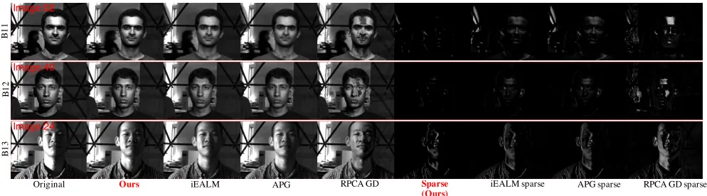
Image:02
Image:40
Image:24
B1
1
B1
2
B1
3
Original Ours iEALM APG RPCA GD Sparse
(Ours) iEALM sparse APG sparse RPCA GD sparse
Figure 5: Shadow and specularities removal from face images captured under varying illumination and camera position. Our feasibility approach provides comparable reconstruction to that of iEALM and APG.
0 0.1 0.2 0.3 0.4 0.5 0.6 0.7 0.8 0.9 1 0
0.1 0.2 0.3 0.4 0.5 0.6 0.7 0.8 0.9 1
(a)
0 0.1 0.2 0.3 0.4 0.5 0.6 0.7 0.8 0.9 1 0
0.1 0.2 0.3 0.4 0.5 0.6 0.7 0.8 0.9 1
(b)
Figure 6: Quantitative comparison of foreground recovered by RPCA F and RPCA GD onBasicvideo, frame size
144×176with observable entries: (a)|Ω|= 0.9(m.n), (b)
|Ω|= 0.8(m.n). The performance of RPCA GD drops sig-nificantly as|Ω|decreases. In contrast, the performance of RPCA F stays stable irrespective of the size of|Ω|. See Ap-pendix for description of the metricdϵ(X, Y).
sequences, we define anϵ–proximity ofXandY as
dϵ(X, Y)def= 1
nm
n ∑
i=1 m ∑
k=1
dϵ(Xik, Yik),
where
dϵ(u, v)def=
{
1 |u−v| ≤ϵ,
0 otherwise,
andϵ∈[0,1]is a threshold. Clearly,0≤dϵ(X, Y)≤1,ϵ↦→
dϵ(X, Y)is increasing, andd1(X, Y) = 1. Ifdϵ(X, Y) =α, thenα×100%of pixels in the recovered video are withinϵ distance, in absolute value, from the ground truth. We used ϵ–proximity to plot results in Figure 6 and more quantitative results by using different|Ω|in Appendix.
Removal of shadows. The images of a face exposed to a wide variety of lighting conditions can be approximated accurately by a low-dimensional linear subspace. More specifically, the images under distant, isotropic lighting lie close to a 9-dimensional linear subspace which is known as the harmonic plane (Basri and Jacobs 2003). We used theExtended Yale Face Databasefor our experi-ments (Georghiades, Belhumeur, and Kriegman 2001). We
compared iEALM, APG, and RPCA GD against our al-gorithm. We downsampled each image to a resolution of
120×160and use 63 images of a subject in each test. For APG and iEALM, the same parameters as those used previ-ously were set. For RPCA GD and our method, we set the target rankr= 9and sparsity levelα= 0.1. The qualitative analysis on the recovered images shows that image recon-struction obtained by our feasibility approach is comparable to that by iEALM and APG (see Figure 5). In contrast, the visual quality of the images of a face reconstructed by RPCA GD are poor.
Further experiments. Due to the limitation of the space, we show many of our experimental results in Appendix. First, on synthetic data, we empirically validate the sensitivity of Algorithm 2 with respect to the initialization, the choices ofr, and sparsity levelα; and the effect of the cardinality ofΩfor Algorithm 3. Next, for quantitative experiments on partially observed background estimation, we incorporate more results for different values of|Ω|by using theϵ–proximity metric. Finally, we perform experiments on inlier face detection and galaxy evolution and show the qualitative and quantitative results.
Conclusion
References
A.-Zhu, Z., and Li, Y. 2016. LazySVD: Even faster SVD decomposi-tion yet without agonizing pain. InAdvances in Neural Information Processing Systems, 974–982.
Artacho, F. J. A.; Borwein, J. M.; and Tam, M. K. 2016. Global be-havior of the Douglas–Rachford method for a nonconvex feasibility problem.Journal of Global Optimization65(2):309–327.
Basri, R., and Jacobs, D. 2003. Lambertian reflection and linear subspaces. IEEE Transaction on Pattern Analysis and Machine Intelligence25(3):218–233.
Bauschke, H. H., and Borwein, J. M. 1996. On projection algorithms for solving convex feasibility problems. SIAM review38(3):367– 426.
Bouwmans, T., and Zahzah, E.-H. 2014. Robust PCA via principal component pursuit: A review for a comparative evaluation in video surveillance.Computer Vision and Image Understanding122:22– 34.
Bouwmans, T.; Sobral, A.; Javed, S.; Jung, S. K.; and Zahzah, E.-H. 2017. Decomposition into low-rank plus additive matrices for background/foreground separation: A review for a comparative evaluation with a large-scale dataset. Computer Science Review 23:1–71.
Boyle, J. P., and Dykstra, R. L. 1986. A method for finding pro-jections onto the intersection of convex sets in Hilbert spaces. In Advances in order restricted statistical inference. Springer. 28–47. Brutzer, S.; H¨oferlin, B.; and Heidemann, G. 2012. Evaluation of background subtraction techniques for video surveillance. IEEE Computer Vision and Pattern Recognition1568–1575.
Cai, J. F.; Cand`es, E. J.; and Shen, Z. 2010. A singular value thresholding algorithm for matrix completion. SIAM Journal on Optimization20(4):1956–1982.
Cand`es, E. J., and Plan, Y. 2009. Matrix completion with noise. Proceedings of the IEEE98(6):925–936.
Cand`es, E. J., and Recht, B. 2009. Exact matrix completion via convex optimization.Foundations of Computational Mathematics 9(6):717–772.
Cand`es, E. J., and Tao, T. 2010. The power of convex relaxation: Near-optimal matrix completion.IEEE Transactions on Information Theory56(5):2053–2080.
Cand`es, E. J.; Li, X.; Ma, Y.; and Wright, J. 2011. Robust principal component analysis? Journal of the Association for Computing Machinery58(3):11:1–11:37.
Chandrasekaran, V.; Sanghavi, S.; Parrilo, P. A.; and Willsky, A. S. 2011. Rank-sparsity incoherence for matrix decomposition.SIAM Journal on Optimization21(2):572–596.
Chen, Y.; Xu, H.; Caramanis, C.; and Sanghavi, S. 2011. Robust ma-trix completion and corrupted columns. InProceedings of the 28th International Conference on International Conference on Machine Learning, 873–880.
Cherapanamjeri, Y.; Gupta, K.; and Jain, P. 2017. Nearly optimal robust matrix completion. InProceedings of the 34th International Conference on Machine Learning (ICML), 797–805.
Cherapanamjeri, Y.; Jain, P.; and Netrapalli, P. 2017. Thresholding based outlier robust PCA. InProceedings of the 30th Conference on Learning Theory (COLT), 593–628.
Drusvyatskiy, D.; Ioffe, A. D.; and Lewis, A. S. 2015. Transversality and alternating projections for nonconvex sets. Foundations of Computational Mathematics15(6):1637–1651.
Dutta, A., and Li, X. 2017. Weighted low rank approximation for background estimation problems. InThe IEEE International Conference on Computer Vision Workshops (ICCVW), 1853–1861. Dutta, A.; Gong, B.; Li, X.; and Shah, M. 2017. Weighted singular value thresholding and its application to background estimation. arXiv:1707.00133.
Dutta, A.; Li, X.; and Richt´arik, P. 2017. A batch-incremental video background estimation model using weighted low-rank ap-proximation of matrices. InThe IEEE International Conference on Computer Vision Workshops (ICCVW), 1835–1843.
Dutta, A.; Li, X.; and Richt´arik, P. 2018. Weighted low-rank approx-imation of matrices and background modeling. arXiv:1804.06252. Dutta, A. 2016. Weighted Low-Rank Approximation of Matri-ces:Some Analytical and Numerical Aspects. Ph.D. Dissertation, University of Central Florida.
Georghiades, A.; Belhumeur, P.; and Kriegman, D. 2001. From few to many: Illumination cone models for face recognition under variable lighting and pose.IEEE Transactions on PAMI23(6):643– 660.
Gower, R. M., and Richt´arik, P. 2015. Randomized iterative meth-ods for linear systems. SIAM Journal on Matrix Analysis and Applications36(4):1660–1690.
Halko, N.; Martinsson, P.-G.; and Tropp, J. A. 2011. Finding structure with randomness: Probabilistic algorithms for constructing approximate matrix decompositions.SIAM review53(2):217–288. He, J.; Balzano, L.; and Szlam, A. 2012. Incremental gradient on the Grassmannian for online foreground and background separation in subsampled video.IEEE Computer Vision and Pattern Recognition 1937–1944.
Hesse, R., and Luke, D. R. 2013. Nonconvex notions of regularity and convergence of fundamental algorithms for feasibility problems. SIAM Journal on Optimization23(4):2397–2419.
Jain, P., and Netrapalli, P. 2015. Fast exact matrix completion with finite samples. InProceedings of The 28th Conference on Learning Theory (COLT), 1007–1034.
Jain, P.; Netrapalli, P.; and Sanghavi, S. 2013. Low-rank matrix completion using alternating minimization. InProceedings of the Forty-fifth Annual ACM Symposium on Theory of Computing, 665– 674.
Jolliffee, I. T. 2002. Principal component analysis. Second edition. Kaczmarz, S. 1937. Angenaherte auflosung von systemen linearer gleichungen. Bulletin International de l’Acad´emie Polonaise des Sciences et des Lettres, A35:355–357.
Keshavan, R.; Montanari, A.; and Oh, S. 2010. Matrix completion from a few entries. IEEE Transactions on Information Theory 56(6):2980–2998.
Lewis, A. S., and Malick, J. 2008. Alternating projections on manifolds.Mathematics of Operations Research33(1):216–234. Lewis, A. S.; Luke, R.; and Malick, J. 2009. Local linear conver-gence for alternating and averaged non-convex projections. Founda-tions of Computational Mathematics9(4):485–513.
Li, P. 2013. Nth element. https://www.mathworks.com/ matlabcentral/fileexchange/29453-nth-element.
Lin, Z.; Ganesh, A.; Wright, J.; Wu, L.; Chen, M.; and Ma, Y. 2009. Fast convex optimization algorithms for exact recovery of a corrupted low-rank matrix. UIUC Technical Report UILU-ENG-09-2214.
Mareˇcek, J.; Richt´arik, P.; and Tak´aˇc, M. 2017. Matrix comple-tion under interval uncertainty.European Journal of Operational Research256(1):35 – 43.
Mateos, G., and Giannakis, G. 2012. Robust PCA as bilinear de-composition with outlier-sparsity regularization.IEEE Transaction on Signal Processing60(10):5176–5190.
Musco, C., and Musco, C. 2015. Randomized block Krylov methods for stronger and faster approximate singular value decomposition. InAdvances in Neural Information Processing Systems, 1396–1404. Necoara, I.; Richt´arik, P.; and Patrascu, A. 2018. Randomized projection methods for convex feasibility problems: conditioning and convergence rates.arXiv preprint arXiv:1801.04873. Netrapalli, P.; Niranjan, U. N.; Sanghavi, S.; Anandkumar, A.; and Jain, P. 2014. Non-convex robust PCA. InAdvances in Neural Information Processing Systems 27. 1107–1115.
Pang, C. H. J. 2015. Nonconvex set intersection problems: From projection methods to the newton method for super-regular sets. arXiv:1506.08246.
Rodriguez, P., and Wohlberg, B. 2016. Incremental principal com-ponent pursuit for video background modeling.Journal of Mathe-matical Imaging and Vision55(1):1–18.
Shamir, O. 2015. A stochastic PCA and SVD algorithm with an exponential convergence rate. InInternational Conference on Machine Learning, 144–152.
Sobral, A., and Vacavant, A. 2014. A comprehensive review of background subtraction algorithms evaluated with synthetic and real videos.Computer Vision and Image Understanding122:4 – 21. Strohmer, T., and Vershynin, R. 2009. A randomized Kaczmarz al-gorithm with exponential convergence.Journal of Fourier Analysis and Applications15(2):262.
Tao, M., and Yang, J. 2011. Recovering low-rank and sparse components of matrices from incomplete and noisy observations. SIAM Journal on Optimization21(1):57–81.
Wang, N.; Yao, T.; Wang, J.; and Yeung, D.-Y. 2012. A probabilistic approach to robust matrix factorization. InProceedings of 12th European Conference on Computer Vision, 126–139.
Waters, A. E.; Sankaranarayanan, A. C.; and Baraniuk, R. 2011. SpaRCS: Recovering low-rank and sparse matrices from compres-sive measurements.Proceedings of 24nd Advances in Neural Infor-mation Processing systems1089–1097.
Wright, J.; Peng, Y.; Ma, Y.; Ganseh, A.; and Rao, S. 2009. Robust principal component analysis: Exact recovery of corrupted low-rank matrices by convex optimization.Proceedings of 22nd Advances in Neural Information Processing systems2080–2088.
Xu, J.; Ithapu, V. K.; Mukherjee, L.; Rehg, J. M.; and Singh, V. 2013. Gosus: Grassmannian online subspace updates with structured– spar-sity. InIn Proceedings of IEEE International Conference on Com-puter Vision, 3376–3383.
Yi, X.; Park, D.; Chen, Y.; and Caramanis, C. 2016. Fast algo-rithms for robust PCA via gradient descent. Advances in Neural Information Processing systems361–369.
Yuan, X., and Yang, J. 2013. Sparse and low-rank matrix de-composition via alternating direction methods.Pacific Journal of Optimization9(1):167–180.
Zhang, T., and Yang, Y. 2017. Robust PCA by manifold optimiza-tion. arXiv:1708.00257v3.